HAL Id: hal-01059010
https://hal-onera.archives-ouvertes.fr/hal-01059010
Submitted on 29 Aug 2014
HAL is a multi-disciplinary open access
archive for the deposit and dissemination of
sci-entific research documents, whether they are
pub-lished or not. The documents may come from
teaching and research institutions in France or
abroad, or from public or private research centers.
L’archive ouverte pluridisciplinaire HAL, est
destinée au dépôt et à la diffusion de documents
scientifiques de niveau recherche, publiés ou non,
émanant des établissements d’enseignement et de
recherche français ou étrangers, des laboratoires
publics ou privés.
Turbulence Model Comparison for Compact Plate Heat
Exchanger Design Application.
F. Vitillo, L. Cachon, P. Millan, P. Reulet, E. Laroche
To cite this version:
F. Vitillo, L. Cachon, P. Millan, P. Reulet, E. Laroche. Turbulence Model Comparison for Compact
Plate Heat Exchanger Design Application.. International Congress on Advances in Nuclear Power
Plants (ICAPP 2014), Apr 2014, CHARLOTTE, United States. �hal-01059010�
Proceedings of ICAPP 2014 Charlotte, USA, April 6-9, 2014 Paper 14143
Turbulence Model Comparison for Compact Plate Heat Exchanger Design
Application
Francesco Vitillo1,2,*, Lionel Cachon1, Pierre Millan2, Philippe Reulet2, Emmanuel Laroche2
1CEA Cadarache, 2 ONERA Toulouse 1
DEN/CAD/DTN/STPA/LCIT, Bât.204 13108 Saint-Paul-lez-Durance, FRANCE
2 ONERA – The French Aerospace Lab, F- 31055 Toulouse, FRANCE
Tel:* +33 (0) 4 42 25 70 66 , Email:* francesco.vitillo@cea.fr
Abstract
In the framework of the Gas-Power Conversion System for the Advanced Sodium Technological Reactor for Industrial Demonstration (ASTRID) project design, works done at CEA are focused on the design of the sodium-gas heat exchanger. Compact plate heat exchangers are indicated as the most suitable technology for such applications.
An innovative compact heat exchanger geometry is proposed in this paper: its innovation consists in creating a 3D mixing flow. The proposed geometry has also very good mechanical resistance to high pressure gradients, being suitable for a large variety of flow applications.
The flowfield inside such a channel is experimentally studied using the Laser Doppler Velocimetry (LDV) technique. The main velocity, the radial velocity as well as the Reynolds stresses are measured: data show the high level of flow mixing and the 3D flow pattern inside the channel. The experimental measurements are then used to validate turbulence models: in particular Reynolds-Averaged Navier-Stokes (RANS) equations are closed using both isotropic 2-equation isotropic eddy viscosity models and a Non-Linear Eddy Viscosity Model (NLEVM).
Presented results represent the first step in the assessment of innovative high-performance compact plate heat exchangers that can be used to increase the plant efficiency as well as decrease the capital cost of the single component.
I. INTRODUCTION The ASTRID project is a French project aiming to
build a GEN IV sodium fast reactor to burn minor actinides, to extend the availability of natural uranium resources still maintaining a safety and security level at least equal to that of current generation nuclear reactors1. The sodium-water chemical interaction being one of the major issues for a safe operation of a SFR, a gas Brayton cycle has been investigated2 to de facto eliminate the occurrence of such an accident. In particular, the best suited gas was found to be the nitrogen, having the best trade-off between plant efficiency and technological use. A number of studies has been done3 to evaluate the R&D program necessary to develop the sodium-gas heat exchanger, which is the critical component substituting the steam generator.
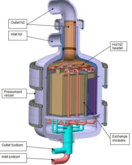
Conceptual designs of compact sodium-gas heat exchanger (SGHE) have been proposed4 (Figure 1) based on existing technologies such as the PCHE and the PSHE. Nitrogen has been chosen as the reference gas for such an application5.
The principle of the Sodium-Gas heat exchanger is to dispose modules of plates in a pressurized vessel which is also the header of the modules. The inlet/outlet of the nitrogen is located on the top of the component and the inlet/outlet of the sodium is on the bottom. More details can be found in reference6. The main issue of this development is to have the highest thermal compactness, and so the judicious choice of the gas flow pattern.
The literature showed how the more 3-D the flow is, the higher is the heat transfer coefficient. Hence, in order to increase the heat transfer coefficient (and the global compactness) the objective is to develop an innovative channel: specifically the channel is composed by elementary geometrical elements like bends, straight channels and mixing zones. Note that there is no available heat exchanger composed by such geometrical elements.
Figure 1 – Conceptual Design of the SGHE A preliminary investigation made at CEA (based on RANS CFD computations) showed that the proposed double channel compact heat exchanger provides a higher compactness (expressed as the thermal power per unit volume of the component) than a commercial PCHE for the same thermal power and pressure drop, as Figure 2 shows.
Figure 2 – Heat Transfer geometry compactness comparison
Hence, the need for a large database of fluid flow inside such a channel is of primary importance to validate the numerical model as well as the performance comparison with other heat transfer geometries.
The innovative channel is therefore the object of the present study. First of all some experimental measurements are shown that are a small part of the database collected. Then, based on the experimental data, a turbulence model validation is performed in order to
determine the most appropriate turbulence model to reproduce the characteristics of the actual flow. Note that the goal of the present paper is not to describe and explain in detail the physics of the flow but rather to validate a model against acquired experimental data. Moreover, as a first step, the current work does not take into account heat transfer inside the innovative geometry, being a pure aerodynamic validation.
II. EXPERIMENTAL MEASUREMENTS
II.A. Experimental setup
In order to show the primary and secondary fluid motion as well as the boundary layer behavior both for the in-bend and the mixing-zone flow, a LDV has been evaluated as the best measurement technique. In particular, due to its capability to measure boundary layers, a 2-C LDV setup has been used to measure the principal and the radial velocity. The experimental setup has been assembled at the ONERA-Toulouse center. The measurement chain is shown in Figure 3:
Figure 3 – LDV Experimental setup
The used technical means are a Spectra Physics Stabilité 2017 Laser, a TSI Colorburst Multicolor Beam Sepatator Model 9201 (both of them shown in Figure 4) to split blue and green beams used for the 2-C velocimetry and to provide the Bragg frequency shifting), an ISEL displacing system, a TSI Colorlink Plus Multicolor Receiver Model 9230 (to measure the laser reception frequency shifting) and a TSI FSA4000 Multibit Digital Processor (to provide digital data to the post-processing computer). The visualization particles are Di-Ethyl-Hexyl-Sebacat (DEHS) droplets.
Figure 4 – Laser and Beam Separator
[M W /m 3] 15 18 17 16
Details on the laser beams are shown in Table I, whereas a view of the measurement volume is shown in Figure 5:
TABLE I Laser Beams Data
Data/Color Green Blue
Wavelength [nm] 514.5 488.0
Beam Diameter [μm] 90.42 85.76
Beam intersection major dimension [mm] 1.32 1.25
Fringe Spacing [μm] 3.70 3.52
Bragg Frequency [MHz] 10 10
Figure 5 – Measurement Volume
The test section is composed by structural aluminum parts with glass windows where the LDV measurement is performed (see Figure 5).
The working fluid is air at atmospheric temperature and pressure. The inlet velocity is 13 m/s, to have a correspondent inlet Reynolds number of 50 600.
II.B. Measurements description
The full measurement campaign has been done on several channel cross sections in the bends as well as in the mixing zone. For the sake of space we will only discuss about a few of them, specifically two profiles in a bend and one profile in the mixing zone. The in-bend profiles lie in a plane having a 45° angular rotation from the bend inlet section. Refer to dotted lines in Figure 6 for their definition of line #1 and line #2:
Figure 6 – In-Bend profiles definition
The mixing zone profiles are defined by dot #3 in Figure 7. Note that the profile is actually along the Y axis normal to the paper XZ plane.
Figure 7 – Mixing zone profiles definition
II.C. Uncertainty evaluation
Three types of uncertainties have been identified during the experimental campaign, specifically the uncertainty due to the data acquisition chain, the uncertainty due to environmental conditions and the uncertainty due to the measurement volume position. Regarding the data acquisition chain uncertainty, the global system calibration gave a velocity standard deviation value never greater than 0.25% of the measured velocity. In order to evaluate the experimental uncertainties in our measurements, two specific tests have been made: first, to be able to quantify the influence of external parameters such as low frequency velocity fluctuations, optical quality of the test section all over the measurements, in-day temperature variations etc. we performed a repeatability test consisting in repeating several times (i.e. around 400 times for the in bend flow and around 200 times for the mixing zone flow) the measurement at the same position. Once collected this data, the uncertainty in the velocity has been calculated as the standard deviation of the sample with regard to the test mean value. Finally, to evaluate the uncertainty due to the measurement volume position, measurements have been done in the vertices of a cube centered in the reference point having the vertices at + 0.2 mm from the center along the three axes X, Y, Z.
The final velocity uncertainty is calculated adding the three obtained variance, calculated as the 3σ where σ is the combined standard deviation determined by adding the variances of each source of uncertainty.
The final uncertainty analysis is shown in Table II and Table III. Note that the evaluation is strictly valid only for the points where the repeatability and the position uncertainty tests have been performed; nevertheless it gives a good idea of the global uncertainties for the actual flow.
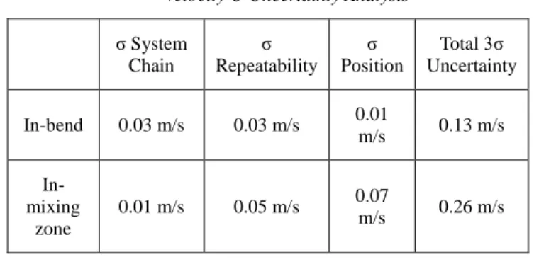
TABLE II
Velocity U Uncertainty Analysis
σ System Chain σ Repeatability σ Position Total 3σ Uncertainty In-bend 0.03 m/s 0.03 m/s 0.01 m/s 0.13 m/s In-mixing zone 0.01 m/s 0.05 m/s 0.07 m/s 0.26 m/s TABLE III
Velocity W Uncertainty Analysis
σ System Chain σ Repeatability σ Position Total 3σ Uncertainty In-bend 0.001 m/s 0.05 m/s 0.14 m/s 0.45 m/s In-mixing zone 0.01 m/s 0.05 m/s 0.07 m/s 0.26 m/s TABLE IV
uw Reynolds Stress Uncertainty Analysis
σ System Chain σ Repeatability σ Position Total 3σ Uncertainty In-bend 0.06 m2/s2 0.04 m2/s2 0.05 m2/s2 0.26 m 2 /s2 In-mixing zone 0.04 m2/s2 0.19 m2/s2 0.14 m2/s2 0.72 m 2/s2
Note that the position uncertainties are quite high and are responsible for a large part of the total uncertainty: indeed these high values are due to the high velocity gradients (hence the large amount of turbulence) in the fluid flow.
III. NUMERICAL VALIDATION
III.A. Turbulence model description
Three turbulence models have been used to test their ability to correctly represent the fluid flow inside the channel. In particular two isotropic eddy viscosity models (e.g. Realizable k-ε and k-ω SST), and a NLEVM will be compared. FLUENT ® code has been used to perform calculations. Since the eventual goal of the study is to use a cost-effective numerical model for the design the
innovative heat exchanger, only two-equation RANS model are evaluated. Hence more complex models such as the Reynolds Stress Transport (RSM) models are out of the scope of this work.
The Realizable k-ε model was proposed firstly by Shih et al.7. The transport equations of the turbulent variables for an incompressible flow are:
�� + (�� ) = [ +�� � ] + − � � + (� ) = [( + � �) ] + +� − � � + √ = � ��
Where Gk is the turbulence kinetic energy production
term. To be consistent with the Boussinesq hypothesis:
= −�̅̅̅̅̅̅′ ′ =
with S being the modulus of the mean rate of strain tensor, defined as follows:
= √
The model is closed by the eddy viscosity formulation, where � is defined as :
�=
� + � � �∗
Where �∗= √ + Ω̅̅̅̅ Ω̅̅̅̅̅ ,
� = . , � = √ cos �, � = cos− (√ �),
� = ̃ and ̃= √ The coefficient is expressed as:
= � [ . ,� + ] ,� � = �
The model constants are:
= . , � = . and ��= . .
To allow for integration up to the wall a Two-Layer Formulation is used: in particular, given the turbulent
Reynolds number � =� √
� , for a Rey > 200 the
complete k-ε model is employed, i.e. both the transport
equation for k and for ε are solved. For Rey < 200 only
the k-transport equation is solved, whereas the turbulence dissipation rate is calculated by a mixing length ℓℇ evaluation as follows:
=� ⁄
ℓ� , ℓ�= ℓ
∗( − �− �⁄��)
The eddy viscosity is damped from the fully turbulent to the buffer region value by the following expression:
, �= � + − � ,� ,
,� = � �ℓ�√�, ℓ�= ℓ∗( − �− �⁄��),
� = [ + tanh ( � −� )]
The model constants are:
ℓ∗= �− ⁄ , = . , �� = ℓ∗, ��= ,
� = .
The Shear Stress Transport (SST) model has been proposed by Menter8. Transport equations of the turbulent variables for an incompressible flow are:
�� + (�� ) = [( + � ) �] + +̃ − � ∗�
� + (� ) = [( + � ) ] + + − � +
The turbulent Prandtl numbers for k and ω are
expressed in the following way:
� = � , + − �, � = � , + − � ,
The function F1 is computed as:
= tanh � , � = � [ � . 9√ ,� � ,��, �� �+ ] (20) + = � [ � � , � , − ]
The turbulence kinetic energy production term in the SST models has a limiter, defined as:
̃ = � , � ∗�
Where Gk is given by Eq.4.
The specific dissipation rate production is given by:
=� ̃, = ∞, + − ∞, ,
∞, = ,∗ −
� , √ ∗,
∞, = ,∗ −
� , √ ∗
The coefficient β is expressed by : = , + − ,
The Cross-Diffusion term Dω is expressed as follows:
= − � �
,
�
Finally the model is closed by the definition of the eddy viscosity:
=��
� [ , � ]
= tanh � , � = � . √� , �
Model constants are:
�, = . , � , = . , � , = . , � , =
. , ∗= . , � = . ,
, = . , , =
. .
With regard to the NLEVM, the adopted model is that of Baglietto et al.9(which has been implemented in FLUENT® via specific User Defined Functions). In particular this is a modified version of the Shih-Zhou-Lumley NLEVM10, where the � value is no longer constant (like in the Realizable k-ε model) but it is expressed as a function of the shear invariant due to realizability constraints:
�= . + ⁄
This time S is the strain invariant, e.g.:
Moreover, the Reynolds stress tensor is expressed as follows:
�̅̅̅̅̅̅ = �� −′ ′ + �[ − ]
+ �[Ω + Ω ]
+ �[Ω Ω − Ω Ω ]
The formulation of the coefficient C1, C2 and C3 is:
= �� �� + �� � = �� �� + �� � = �� �� + �� �
The values of the constants CNL1, CNL3, CNL3, CNL4 and CNL5 are shown in Table V:
TABLE V NLEVM coefficients Constant Value CNL1 0.8 CNL2 11.0 CNL3 4.5 CNL4 1000.0 CNL5 1.0
The non-linear eddy viscosity formulation is then coupled with the standard k-ε model of Launder and Spalding7. Note that the anisotropies and the realizability conditions for the present model are included in the new Reynolds stress tensor definition. The near-wall treatment is the same as the Realizable k-ε model, i.e. the Two-Layer formulation previously described.
III.B. Boundary condition and meshing convergence evaluation
Three different meshing configurations have been preliminarily studied in order to evaluate the influence of mesh size on the solution. The three unstructured mesh configurations (hereafter named as A, B, C) differ by a factor of around 2 on the mesh size in the first layer thickness and in the global size of a single mesh cell:
TABLE VI Mesh Description Configuration First Layer Thickness Major Size of a single Element Number of Nodes A 1x10⁻⁴ m 5x10⁻³ m 2,274,099 B 5x10⁻⁵ m 4x10⁻³ m 4,179,540 C 3x10⁻⁵ m 3x10⁻³ m 9,349,932
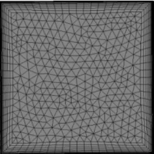
Values of the average wall y+ are about 2.8, 1.4 and 0.8 respectively for configuration A, B and C. Meshing has been done using the ANSYS® Mesh module: an example of the inlet section mesh for the C configuration is shown in Figure 8:
Figure 8 – Inlet section mesh for C configuration A 13 m/s velocity inlet (Dirichlet) and a gauge pressure equal to 0 Pa pressure outlet (Neumann) boundary conditions are used. The working fluid is air at atmospheric temperature and pressure. The solver is the Pressure-based one and the Coupled pressure-velocity algorithm with pseudo-transient option is used. Gradients are evaluated through the Green-Gauss node-based method. Finally the Second Order Upwind Scheme is used for the spatial discretization of momentum, turbulent kinetic energy, turbulent dissipation rate (for the Realizable k-ε and the NLEVM models) or the specific dissipation rate (for the SST model).
Meshing convergence has been evaluated by comparing the average wall shear stress on the walls of the channel.
Table VII shows the results of the convergence evaluation for the three models:
TABLE VII
Average wall shear stress convergence evaluation
Configuration Realizable
k-ε SST NLEVM A 0.940 Pa 1.001 Pa 0.948 Pa B 0.916 Pa 0.984 Pa 0.923 Pa C 0.917 Pa 0.988 Pa 0.910 Pa From values in Table VI see that configuration C shows a converged wall shear stress solution both for Realizable k-ε and SST model and a difference of about 1.5% in the average wall shear stress for the NLEVM model. Based on these trends, we retained configuration C as the reference meshing, a finer grid leading to numerically unstable calculations, especially for the NLEVM.
III.C. Comparison with experimental data
A first model validation is done on the channel pressure drop (Table VIII):
TABLE VIII
Pressure Drop model validation LDV or
Model Value [Pa] LDV 488 + 20
k-ε Real. 557.4
SST 549.3
NLEVM 512.4
The NLEVM model seems to provide a good pressure drop evaluation. Nevertheless it is worth analyzing the collected LDV data in order to better understand the most appropriate model to simulate the flow inside the channel.
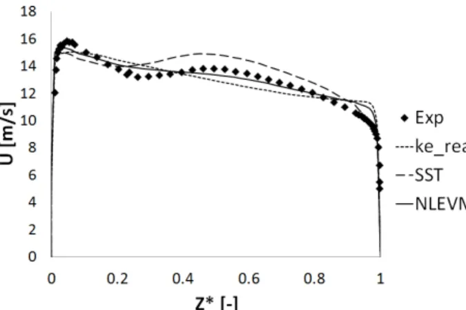
With regard to the geometrical details given in Figure 6 and Figure 7 we are going to show the measurements of the X-velocity (hereafter “U”), Z-velocity (hereafter “W”) and XZ-Reynolds stress (hereafter “uw”). Figure 9 to Figure 17 show the comparison between experimental LDV data and numerical calculations with the three models previously described. Note that abscissas are non-dimensional coordinates (Y* and Z*) for the region of interest. In particular for the mixing zone the middle-plane (i.e. the middle-plane where mixing occurs) is in Y*=0.5.
Figure 9 – U velocity comparison in line #1
Figure 10 – W velocity comparison in line #1
Figure 11 – uw Reynolds Stress comparison in line #1
Figure 13 – W velocity comparison in line #2
Figure 14 – uw Reynolds Stress comparison in line #1
Figure 15 – U velocity comparison in line #3
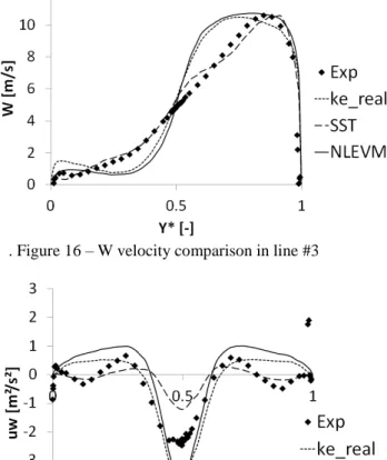
. Figure 16 – W velocity comparison in line #3
Figure 17 – uw Reynolds Stress comparison in line #1
As a general consideration, see that the SST model give the best overall results compared to the other models. As regards the in-bend flow, the SST model seems to provide very good results. Principal U velocity as well as radial W velocity profiles are very well calculated. On the other hand the uw Reynolds stress is generally under-predicted, still having a good global trend. The Realizable k-ε and the NLEVM model cannot reproduce the actual flow as precisely as the SST model.
The principal reasons are to be found in the fact that
the ε-based formulation of the Realizable k-ε and the
NLEV models is known not to work properly for adverse pressure gradient flows11. Moreover the SST eddy viscosity formulation is known to give very good results for adverse pressure gradient boundary layers: in fact, even though the NLEVM model: in fact, even though the NLEVM model has an improved eddy viscosity
formulation (i.e. through the variable Cμ), it is supposed
to assure global model realizability rather than improve adverse pressure gradient boundary layers. For an in-bend flow this seems to be a critical deficiency. See Figure 18 to analyse the eddy viscosity distribution in the outer bend boundary layer in line 1:
Figure 18 – Outer bnd boundary layer Eddy viscosity comparison in line#1
While the eddy viscosity in the viscous sublayer is quite the same for the three models (being a small fraction of the molecular viscosity in this region), differences appear in the outer boundary layer. There is a factor of about two between the eddy viscosity calculated by the Realizable k-ε and the NLEV models and the one calculated by the SST. See indeed the high velocity gradient eddy viscosity limiter in the SST formulation, which seems to act very well in the near wall region; this is not necessarily true for the Realizable k-ε and the NLEV models. Hence it appears that the formulation of the eddy viscosity used in a very similar way in the Realizable k-ε and the NLEV model (Eq. 6 and Eq.32) gives very similar results but does not work properly, at least for adverse pressure gradient flows.
As regards the mixing zone, first of all note that there are two isolated points in the boundary layer at Y*≈1 both in Figure 15 and Figure 17: they are likely spurious experimental points where the LDV system measured a false value either due to proximity to the glass window or to a DEHS spot deposed in the glass window. Anyway the SST model correctly represents the two velocity components U and W and gives a good trend for the uw Reynolds stress. Concerning the Realizable k-ε and the NLEVM model, the velocity profiles are not in good agreement with the experimental data and the uw stress, although it is good regarding the global range of values, does not have the right trend in the near middle-plane (Y*=0.5) region as well as in the near-wall region. A possible explanation for this behaviour likely lays again in the turbulence kinetic energy production term (Eq.29): this production limiter is supposed to make the model quasi-realizable, setting a necessary upper bound on the turbulence kinetic energy production term as shown by Durbin12.
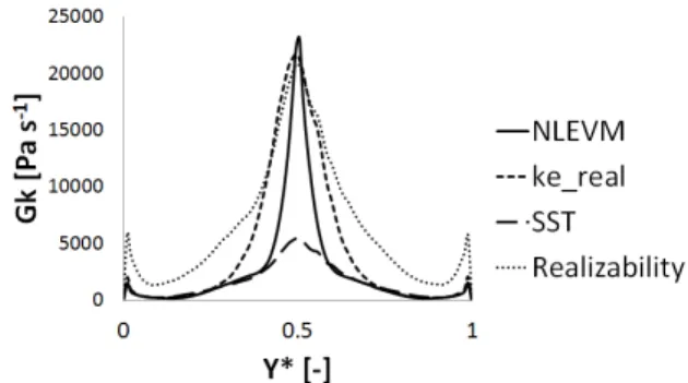
See in Figure 19 the turbulence kinetic energy production profiles in the three models:
Figure 19 – Turbulence Kinetic Energy Production term comparison in line#3
Together with the turbulence kinetic energy production term for the three used models, a Realizability plot is also shown, based on the upper bound proposed by Durbin12 and Park and Park13. An actual improvement in the modelling of this term seems to be the limiter in the SST model. This limiter is supposed to improve the model behaviour in stagnation points14: indeed the mixing zone middle plane seems to represent a zone of turbulence kinetic energy build-up due to the counter-converging two flows. Indeed all the three models respect the Realizablity condition; nevertheless, the SST model is the only one that do not reach the Realizability-imposed limit in the middle of the mixing zone. Therefore the higher turbulence kinetic energy production both for the Realizable k-ε and the NLEV model in this zone provides an excessive turbulence kinetic energy, which gives a too much high value of the eddy viscosity along the Y direction: this results in a higher flow diffusion along the X and Z directions limiting the flow penetration along Y direction. This finally results in a more typical “all-alone” flow profile (e.g. not enough mixing), as those of Figure 15 and Figure 16.
IV. CONCLUSIONS
From this analysis it can be stated that the SST model gives very satisfactory results for the complex flow presented, even being a RANS two-equation model: it provides a good description of the fluid flow and a slight pressure drop overestimation. The Realizable k-ε almost never gives the good trends, still suffering the well-known deficiencies of all k-ε based models. The NLEVM formulation coupled with the Standard k-ε model works slightly better than the Realizable k-ε model, giving a good prediction of the pressure drop but still presenting many deficiencies regarding the fluid flow description. In particular the major features providing such good results for the SST model seem to be the good in-bend flow
descrption given by an ω-based model (like the SST), the
turbulence kinetic energy production limiter and the eddy viscosity formulation: they actually prevent the turbulence kinetic energy build-up that provides an erroneous prevision of both in-bend and mixing zone when
Realizable k-ε and the NLEV models are used. Moreover, despite the fact that an non-isotropic model would be supposed to give better results for such a complex flow, this seems not to be the case if the non-isotropic model cannot correctly represent the global flow inside the different parts of the channel (in this case the k-ε model cannot correctly represent the in-bend flow).
Indeed the results given by the SST model are valuable considering the complexity of this wall-bounded flow. Hence its utilisation is strongly recommended for the description and the following numerical studies in the present geometrical configuration.
ACKNOWLEDGMENTS
This work is done within a PhD collaboration between the CEA-Cadarache center and the ONERA – Toulouse Center. The authors want to thank Mr. Christian Pelissier, Mr.Francis Micheli and Mr.Jean-François Breil for the valuable help in setting and operating the LDV system.
NOMENCLATURE CFD: Computational Fluid Dynamics
ASTRID: Advanced Sodium Technological Reactor for Industrial Demonstration
GENIV: Generation IV International Forum SFR: Sodium-cooled Fast Reactor
PCHE: Printed Circuit Heat Exchanger PSHE: Plate Stamped Heat Exchanger 2-C: 2 component (i.e. of velocity vector) LDV: Laser Doppler Velocimetry
σ: Standard deviation for a statistical distribution
Ui: i-mean velocity component
ui: i-fluctuating velocity component
ρ: Fluid density
k: Turbulence kinetic energy (TKE)
μ: Molecular dynamic viscosity μt: Eddy viscosity
ε: Turbulence dissipation rate (TDR) σk: TKE Prantdl number
σε: TDR Prantdl number
ω: Specific dissipation rate (SDR) σω: SDR Prantdl number
y: distance to the nearest wall
= �� + �� Deformation rate
Ω = �� − �� Rotation rate
Y+: non-dimensional distance from the wall REFERENCES
1. CEA, “ASTRID une option pour le nucléaire du
futur”, Les Défis du CEA, 172 (2012)
2. M.SAEZ et al., “The Use of Gas Based Energy
Conversion Cycles for Sodium Fast Reactors”,
Proceedings of the 2008 International Conference on the Advances in Nuclear Power Plants – ICAPP’08,
Anaheim (CA) USA, June 08-12, 2008 Paper 8037 3. L.CACHON et al., “Innovative Power Conversion
System for the French SFR Prototype ASTRID”,
Proceedings of the 2012 International Conference on the Advances in Nuclear Power Plants – ICAPP’12,
Chicago (IL) USA, June 24-28, 2012 Paper 12300 4. L.CACHON et al., « Preliminary Design of a Large
Scale Sodium Gas Heat Exchanger (SGHE) for the Nitrogen Power Conversion System envisaged for the
ASTRID SFR Prototype”, International Conference
on Fast Reactors and Related Fuel Cycles: Safe Technologies and Sustainable Scenarios (FR13),
Paris (France), March 4-7,2013 Paper 118
5. N.ALPY et al., “Gas Cycle Testing Opportunity with ASTRID, the French SFR Prototype”, Supercritical
CO2 Power Cycle Symposium, Boulder (CO) USA,
May 24-25, 2011
6. L.CACHON et al., PATENT n°HD14482
7. T.H.SHIH et al., “A New k-ε Eddy Viscosity Model for High Reynolds Number Turbulent Flows – Model Development and Validation”, Computers and Fluids, 24, 3, 227-238, 1995
8. F.R.MENTER, “Two-Equation Eddy-Viscosity
Turbulence Models for Engineering Application”,
AIAA Journal, 32, 8, 1598-1605 (1994)
9. E.BAGLIETTO, H.Ninokata and T.Misawa, “CFD and DNS methodologies development for fuel bundle
simulations,” Nuclear Engineering and Design, 236,
1503-1510 (2006)
10. T.H.SHIH, J.Zhu and J.L.Lumley, “A Realizable
Reynolds Stress Algebraic Equation Model”, NASA
TM 105993 (1993)
11. D.C.WILCOX, Turbulence Modeling for CFD, Third
Edition, DCW Industries, 2006
12. P.A.DURBIN, “Limiters and wall treatments in
applied Turbulence”, Fluyd Dyn. Res., Invited
Review, 41, 2009
13. C.H. PARK and S.O.Park, “On Limiters of
two-equation turbulence models”, International Journal
of Computational Fluid Dynamics, 13,1, 79-86
(2006)
14. F.R.MENTER, “Zonal Two-Equation k-ω Turbulence Models for Aerodynamic Flows”, AIAA Paper