HAL Id: hal-00945515
https://hal.inria.fr/hal-00945515
Submitted on 12 Feb 2014
HAL is a multi-disciplinary open access
archive for the deposit and dissemination of sci-entific research documents, whether they are pub-lished or not. The documents may come from teaching and research institutions in France or abroad, or from public or private research centers.
L’archive ouverte pluridisciplinaire HAL, est destinée au dépôt et à la diffusion de documents scientifiques de niveau recherche, publiés ou non, émanant des établissements d’enseignement et de recherche français ou étrangers, des laboratoires publics ou privés.
Jacques Rubin
To cite this version:
Jacques Rubin. The projective geometry of the spacetime yielded by relativistic positioning systems and relativistic location systems. 2014. �hal-00945515�
Jacques L. Rubin
(email: jacques.rubin@inln.cnrs.fr) Université de Nice–Sophia Antipolis, UFR Sciences
Institut du Non-Linéaire de Nice, UMR7335 1361 route des Lucioles,
F-06560 Valbonne, France
(Dated: February 12, 2014)
As well accepted now, current positioning systems such as GPS, Galileo, Beidou, etc. are not primary, relativistic systems. Nevertheless, genuine, relativistic and primary positioning systems have been proposed recently by Bahder, Coll et al. and Rovelli to remedy such prior defects. These new designs all have in common an equivariant conformal geometry featuring, as the most basic ingredient, the spacetime geometry. In a first step, we show how this conformal aspect can be the four-dimensional projective part of a larger five-dimensional geometry. Our aim has been then to explore and collect all of the geometric, physical consequences of this projective geometry in such spacetime context and ask for a physical process, the implementation of which could reveal this fifth dimension. We find that the latter is physically obtained from a fifth time stamp effectively yielded from a new localization protocol that we present jointly with this projective geometry. Based on this fifth supplementary parameter, beside the four usual ones identified with the four basic time stamps broadcast by any positioning system, we deduce the four-dimensional projective geometry governing spacetime. The former is completely detailed, i.e., the projective Cartan connection and its projec-tive curvature are computed. As a result, the Einstein tensor appears to be algebraically remarkable in this projective context. In particular, this leads to a new surprisingly result in the complete inte-grability of the Einstein equations while the well-known incompleteness of their usual non-projective version is unquestioned. Also, it may validate completely or gives naturally true physical grounds to the old model due Yano, Ohgane and Ishihara or the new approach developed by Bradonjić and Stachel similar to the one due to Schouten, Haantjes and van Dantzig unifying electromagnetism and gravitation in which the homogeneous coordinates remained till now unidentified physically. PACS numbers: 02.10.De , 04.20.-q, 04.20.Cv, 45.10.Na, 91.10.Ws, 95.10.Jk
Keywords: Causal types; Emission coordinates; Lorentzian metric; Relativistic positioning systems
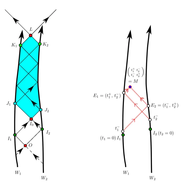
I.2 Figure on the left: the “hexagonal” domain I0J1K1LK2J2I0. Figure on the right: the dashed lines are the light-like paths of the signals carrying the time stamps with values t±
1 and t ± 2 by successive echoes. For instance, at the event E2, we have an echo with the reception of the time stamp with value t−
1 and a sending to M of a pair of time stamps with values (t −
1, t+2).. . . 3
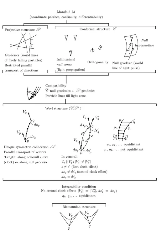
II.1 General scheme of conformal, projective, Weyl, and Riemannian structures (From Fig. 1. in Ehlers-Pirani-Schild paper [EPS72, p.66]) . . . 14
III.1 Schema representing the projective frame Ψ ={(p0,[0]), (ζ1,[+∞]), (p2,[1])}≡{[ζ0], [ζ1], [ζ2]} of the projective space RP1 in R2.. . . 28
IV.1 The Tzitzeica surface Tı2 in R3 with its four strata.. . . 74
VIII.1 The system of echoes in dimension two.. . . 114
VIII.2 The two-dimensional grid.. . . 115
VIII.3 The system of echoes with four past null cones. . . 116
VIII.4 The three data received and recorded by the user at U,Ue andUb.. . . 117
VIII.5 The change of projective frame at E.. . . 120
VIII.6 The event e in the four past null cones of the four events E, E, Ee and Eb. This event e is observed on their respective celestial spheres C, C,CeandC.b . . . 130
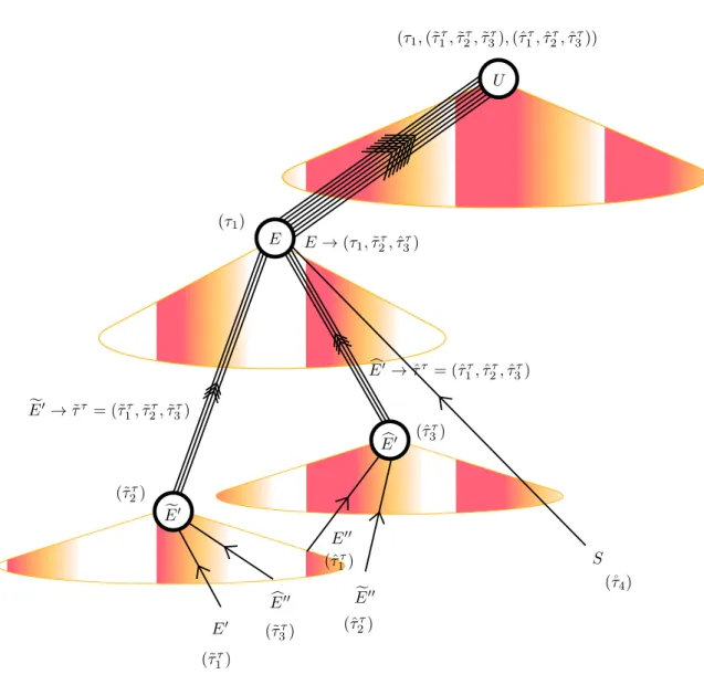
VIII.7 The event E in the five future null cones of the five events e, E′ ,Ee′, b E′ and ˚ E′. . . . 131
VIII.8 An example of successive events ˚E′, ˚E•, ˚E◦ and ˚E∗ on the anchoring worldline of ˚E broad-casting their coordinates ˚τ5 towards the four events E, E,EbandE.e . . . 132
VIII.9 The projective disk at the event E associated to the celestial sphere C of the emitter E.. . . 133
A.1 Protocole de Marzke-Wheeler.. . . 169
A.2 The Marzke-Wheeler principle . . . 170
C.1 △P(r2)with △P(h1h5) < 0. . . 200
C.2 △P(r2)with △P(h1h5) = 0. . . 200
C.3 △P(r2)with △P(h1h5) > 0. . . 201
C.4 The triangle-shaped loop Γ. . . 201
I. Introduction - The Coll-Ferrando-Morales-Tarentola protocols 1
II. The metric and the “energyspacetime” – A fundamental exemple 5
A. A fundamental example 5
B. What is projective or conformal, and in which manifold? 12
III. A short review on the projective differential geometry 18
A. Cartan versus Ehresmann approaches 18
B. The projective manifold and the projective group actions 26
C. The projective Cartan connections 32
1. The general case – Definitions and terminologies 32
2. From Euclidean connections to projective connections and their associated
covariant derivatives 49
3. General properties 59
4. The projective (co-)tensors versus the Euclidean (co-)tensors – General
remarks. 62
5. A fundamental exemple on RPn: the Cartan approach (1924). 66
IV. The three-dimensional submanifolds of MRP S modeled on RP3 70
A. The RP3 projective connections on M
RP S 70
B. The metric fields on MRP S 80
1. An examples of metric field on MRP S 80
2. The metric field g of the spacetime MRP S yielded by relativistic positioning
systems 82
V. The projective curvature 2-form Ω 89
A. The general case on RPn 89
B. The torsion-free and normal projective connections on RPn 95
VII. Interpretations – General remarks 108
VIII. A protocol implemented by receivers to localize events 112
A. The protocol of localization in a (1 + 1)-dimensional spacetime M 113 B. The protocol of localization in a (2 + 1)-dimensional spacetime M modeled on
RP3 114
C. The protocol of localization in a (3 + 1)-dimensional spacetime M modeled on
RP4 128
IX. The geometry of M modeled on RP4 139
A. The metric field defined on M” 139
B. The projective Cartan connection and the Yano-Ishihara projecting 1-form on
”
M 144
1. The projective Cartan connection ω 153
2. The projective geodesic equations 155
3. The projective curvature 2-form and the normal projective Cartan connection 158
4. The metric field from the physical tensors 163
X. Conclusion and interpretations 165
Appendices 169
A. The Marzke-Wheeler protocol 169
B. Proofs of the two “factorization theorems” 171
1. Introduction 171
2. The equivalent generic metric fields 173
a. The systems of equations 174
b. The Pfaff systems and the proof of Theorem B.1 179
C. The “loop degeneracy” 184
1. Introduction 185
2. Generic normal forms of {ssst} or {ℓℓℓℓ} causal types for metrics 187
a. The generic normal forms G⊥ and Gϵ 187
b. The coefficients of G⊥ and Gϵ 191
3. The systems of algebraic equations 192
a. The algebraic system in dimension 4 192
b. The reduced algebraic system in dimension 3 193
4. The domains of algebraic resolution 194
a. The roots if r2= 0 195
b. The roots if r2= h1h5 196
c. The roots if △P(r2) ⩾ 0 with r2∈ ]0, h1h5[ 196
d. The nonnegative domain of △P(r2) with r2 ∈ ]0, h1h5[ 197
5. Examples and “loop” solutions 199
6. Conclusion 205
D. The Sturm sequence of △P(r2) 205
E. The univariate polynomial equations of degree 3 or 4 and their positive roots 207 1. – The discriminant and the roots of polynomial equations of degree 3 207 2. – The discriminant and the roots of polynomial equations of degree 4 208
3. – The signs of the real roots 213
F. The space and time “projective” splitting 217
G. Proof of the 1947 Ehresmann’s Theorem 218
H. Proof of the Theorem 1 229
K. The Christoffel symbols 235 L. The infinitesimal automorphisms of the Yano-Ihsihara projecting 1-form ˆπ 237
M. The Christoffel symbols of ˆg in M” 239
N. The projective geodesics onM” 243
References 249
I. INTRODUCTION - THE COLL-FERRANDO-MORALES-TARENTOLA PROTOCOLS
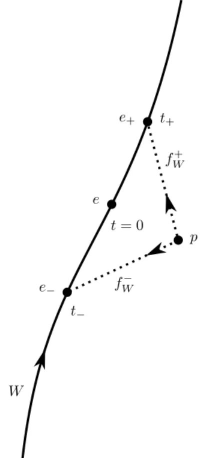
Historically, the most “basic” first tool for positioning events in Minkowski spactime was based on the so-called Marzke-Wheeler protocol [MW64] (see Appendix A). Then, eight years later, Ehlers, Pirani and Schild [EPS72] improved the latter protocol in the framework of the general relativity, and they defined a metric g with a Lorentz signature on a given spacetime manifold M starting from what we call a ‘potential of metric v’ or a ‘distance function v’ on M. The metric g obtained in this way is uniquely defined at any event e ∈ M, up to a conformal factor, from any parameterized time-like worldline W such that e ∈ W and t(e) = 0, where t is any time parameterization given on W (see Figure I.1). One of the essential ingredients in this
e− e+ e p W fW+ fW− t = 0 t+ t−
definition are the so-called ‘radar coordinates’ r+ and r− defined themselves respectively from the so-called ‘message functions’ f+
W and fW−. The latter are maps associating any event p ∈ M with two events e± ∈ W such that e+ (resp. e−) is on the future (resp. past) light cone of p. Then, the radar coordinates are maps from M to R such that r±≡ t ◦ fW± and the potential of metric v is defined by the product of r+ and r−:
v ≡ − r+r−. (1.1)
Then, the metric g is obtained from the Hessian of v or, equivalently, from the following formula:
g ≡ − dr−⊗ dr+− dr+⊗ dr−≡ −2 dr+⊙ dr−, (1.2)
where d is the exterior derivative defined on M and ⊙ represents the symmetrized tensor product. At the event e ∈ W, the metric g is defined up to conformal factors due to any change of parameterization t of W satisfying the constraint t(e) = 0.
Unfortunately, this protocol cannot be really implemented physically because the value t+ = r+(p) of the radar coordinate r+ is obtained by any observer at p from signals coming from the future. To circumvent this difficulty, Coll, Ferrando, Morales and Tarentola proposed an alternative protocol in four-dimensional spacetimes [Col85, Col01a, Col02, CT03] (see also Blagojević et al. [BGHO02], Bahder [Bah01, Bah03, Bah04] and Rovelli [Rov02a, Rov02b]), but also, in particular, primarily in two-dimensional spacetimes [CFM06b, CFM06a, CP06, CFM10a, CFM10b] with at least two worldlines W1 and W2 (see Figure I.2).
With their protocol, only signals coming from the past are utilized to deduce the metric g or the spacetime positions of users in what we call a ‘hexagonal domain’ I0J1K1LK2J2I0 of the spacetime between the two given worldlines W1 and W2. Their protocol can be presented in a simplified version in a two-dimensional spacetime as follows. Let us consider the event O corresponding to an ignition event from which two flashes of light are emitted toward the two time-like worldlines W1 and W2. These two flashes are received on W1 and W2 at the events I1 and I2 respectively and they ignite or set to zero the two parameterizations t1 and t2 given on these two worldlines. Then, the point I0 has the coordinates (t1 = 0, t2 = 0) (see Fig. I.2). Moreover, we consider that the two worldlines are the trajectories of two emitters which send
I2 I1 O W1 W2 J2 L J1 K1 K2 I0 E1= (t + 1, t − 2) E2= (t − 1, t + 2) t− 2 t− 1 I2(t2= 0) (t1= 0) I1 Å t+ 1 t−2 t− 1 t + 2 ã W1 W2 = M
Figure I.2. Figure on the left: the “hexagonal” domain I0J1K1LK2J2I0. Figure on the right: the dashed lines are the light-like paths of the signals carrying the time stamps with values t±
1 and t ±
2 by successive echoes. For instance, at the event E2, we have an echo with the reception of the time stamp with value t−
1 and a sending to M of a pair of time stamps with values (t−1, t+2).
themselves — via light-like paths — time stamps and broadcast continuously those ‘time stamps’ they receive by producing, somehow, echoes.
Then, it can be shown that at any event M in the hexagonal domain, four numbers (t+1, t+2, t−1, t−2) carried by the time stamps can be obtained and utilized by any user at M to build a grid or a chart in the hexagonal domain and to deduce the spacetime positions of M and the two emitters, say E1 and E2 (on W1 and W2), in this grid. In the latter, the event M
has the coordinates t+
1 and t+2, i.e., M ≡ (t+1, t+2), whereas the two emitters have the emission coordinates E1 ≡ (t+1, t−2) and E2 ≡ (t−1, t+2). Moreover, the spatial distance between the two events of ignition I1 and I2 is not defined, but can be posed as a standard of distance associated with the relativistic positioning system defined by the two worldlines W1 and W2. What is really of importance is to be able in this situation to define the protocol putting in correspon-dence the standards associated with two such different positioning systems. Then, by standard matching we may tend possibly toward a limit case with a positioning system composed of two intersecting worldlines for which a standard is not necessary.1 But, as in the Marzke-Wheeler protocol, we can also define a potential of metric v. Indeed, we can take v as the Lorentzian distance function d(O, M) between O and M such that
v ≡ d(O, M) ≡ − t1(fW−1(M )) t2(fW−2(M )) = − t
+
1 t+2 . (1.3)
Then, the metric g is defined by the relation:
g ≡ −2 dt+1 ⊙ dt+2 . (1.4)
In a four-dimensional spacetime, the situation is quite similar with four emitters rather than with two emitters only. But, different approaches can be taken a priori to describe the possible underlying geometry of the spacetime deduced from such protocols. One of them, generalizing the Coll-Ferrando-Morales-Tarentola protocol (CFMT), was investigated by Ferrando and Sáez in the framework of the ‘2 + 2 warped spacetimes’ by duplicating the two-dimensional approach [FS10]. In the present paper, we determine the spacetime geometry deduced from the strict general four-dimensional protocol such as the one described for instance in the so-called SYPOR relativistic positioning system [CT03]. The main goal is, at first, to define a metric g in a four-dimensional spacetime generalizing the formula (1.4) and then, to deduce the spacetime geometry.
1The importance of such an intersection point —the so-called ‘cut event’— of the two worldlines of the two emitters has
II. THE METRIC AND THE “ENERGYSPACETIME” – A FUNDAMENTAL EXEMPLE
A. A fundamental example
Any Lorentzian metric g can be always put univocally in the following general form in a {ℓℓℓℓ}-coframe (ℓ for light):
g = − 4
∑
i<j=1
νiνjdτi⊙ dτj, (2.1)
where the ν’s are positive (nonvanishing) functions depending on four time coordinates τkwhich are the time parameterizations (stamps) of four worldlines travelled by four emitters (see also analogous situations in [KM07, KMW10, KM10, KM12]).
More precisely, we proved the two following theorems (see Appendix B for the proofs) we call the “factorization theorems.” Let πn be the trivial fibration πn : M2 ≡ M×M −→ M, corresponding to the projection onto the first factor and where dim M = n in full generality. We denote by Jk(πn)the fiber bundle of jets of order k ⩾ 0 of the local smooth sections of πn. In particular, we have J0(πn) ≡ M2 with local coordinates (τ, ψ) ≡ (τ1, . . . , τn, ψ1, . . . , ψn) where τ is the source and ψ is the target. Furthermore, let
ψ1 ≡ (τ1, . . . , τn, ψ1, . . . , ψn, ψ11, ψ21, . . . , ψji, . . . , ψnn−1, ψnn)
be a local system of coordinates on J1(πn). We denote also by Πk(πn) ⊂ Jk(πn) the set of invertible elements of Jk(πn), i.e., the set of k-jets of local smooth diffeomorphisms on M. Πk(πn) is a groupoid with source map αk : Πk(πn) −→ M where M is the first factor of M2 and the target map βk : Πk(πn) −→ M where we project onto the second factor. Also, we denote by Πk(πn) the presheaf of germs of local smooth αk-sections of Πk(πn). Then, we consider any solution of the system of PDEs (2.3) below as a sub-manifold of Π1(πn)transversal to the αk-fibers and defined from the following system R1 of equations on the presheaf Π1(πn):
R1: n
∑
r, s=1
grs(ψ) ψri ψjs− ϵijνi(τ ) νj(τ ) = 0 , i, j = 1, . . . , n , (2.2) where νi(τ ) > 0. Then, we have the following first theorem.
Theorem 1. (First factorization theorem). If n ⩽ 4, there always exists a smooth
local diffeomorphism f(τ) = ψ and n smooth positive functions νi(τ ), both defined on an open
neighborhood V ⊂ U of any given point of U, such that for all τ ≡ (τ1, . . . , τn
) ∈ V the relations ˜ gij ≡ n ∑ r, s=1
grs(f )(∂ifr)(∂jfs) = ϵijνiνj, i, j = 1, . . . , n , (2.3)
hold with ϵij =sgn(gij) =sgn(˜gij) whenever i ̸= j and ϵij = 0 otherwise. Then, we say that the
“generic” metric ˜g is ℓ-equivalent to g (through f).
And also, if M is time oriented, i.e., there exists a complete (future time-like) vector field ξ on M, then, we have the following second theorem:
Theorem 2. (Second factorization theorem). If n = 4, then, given a Lorentzian metric
g on M assumed to be time oriented, connected and simply connected, then, there exists only
one smooth diffeomorphism fi(τ ) ≡ ψi being a solution of R
1 of which the Jacobian matrix is
an element of O(4, R); and, as a result, there is a unique set of four positive functions νi. Also,
the unique ℓ-equivalent metric field ˜g is ‘isometrically equivalent’ to g. Then ˜g is said to be
ℓ-isometric to g and ℓ-generic.
It must be noted that not any given Lorentzian metric g can be diagonalized without implicit assumptions if dim M ⩾ 4 . Indeed, we have always an (pseudo-)orthogonal coframe only in a manifold of dimension n less than or equal to 3. We recall that a pseudo-orthogonal coframe is a cobasis of 1-forms σi (i = 1, . . . , n) such that g ≡∑n
i ϵiσi⊙σi and σi∧dσi = 0with ϵi = ±1. The vanishing of the Weyl tensor is, for instance, a sufficient condition in a torsion-free Riemann structure (i.e., the connection on M is the Levi-civita connection) to have such pseudo-orthogonal coframe in dimension n ⩾ 4, and then, to diagonalize g.2
2 Actually, in a given coframe, the necessary and sufficient condition for this coframe to be (pseudo-)orthogonal is the
vanishing of certain coefficients of the Riemann tensor R. More precisely, the coefficients Rij,kℓof the Riemann tensor
must vanish whenever all of the indices i, j, k and ℓ are distinct (a condition always satisfied in dimension less than or equal to 3). This is equivalent to the vanishing of all of the corresponding covariant components of the Weyl curvature tensor (obviously, a vanishing Weyl tensor involves such relations on the Riemann coefficients) [Wei72, see pp. 145– 146][BCG+91, pp. 88–91][Bry99, §7 pp. 46–47]. The proof in [Bry99, §7 pp. 46–47] is given for orthogonal coordinate
charts and Euclidean metrics on R. However, because the proof is analytical, it remains valid on C. We must just consider an Euclidean metric g =∑4
j=1αj⊗ αjon C with αk≡ i
√
|akk| duk for three of the four indices j and, additionally,
keeping the same dimensions of the various varieties or manifolds but on C . See also, for instance, the conclusion P.15 § 4.2 “The Lorentzian case” in [GV09].
It follows, on the contrary, that a nonvanishing Weyl tensor can be compatible with a non-diagonalization whatever are 1-forms σi satisfying σi∧dσi= 0,3 and then, in full generality and without any indication a priori on this vanishing, we cannot recast our geometrical approach starting with a diagonal metric g.4 In particular, applying the well-known Newman-Penrose formalism of “null” tetrads [NP04] we must be aware that the orthogonality condition imposed by Newman and Penrose to their “null” tetrads cannot be satisfied to any set of four null vectors. Moreover, g does not derive, in full generality, from a potential of metric ψ. But, if g admits such potential we should have the following system R2 of partial differential equations (assuming that the roman indices i, j, k, . . . are equal to 1, 2, 3 or 4):
R2≡ ∂ijψ = νiνj if i ̸= j, ∂kkψ = 0, (2.4) where ∂k represents the partial derivative with respect to the time coordinate τk. The symbol M2 of this system of partial differential equations of degree 2 is vanishing, i.e., the system R2 is involutive. Therefore, all the ‘compatibility conditions’ (CC) derive from those obtained from the first prolongation of R2. More precisely, we obtain:
CC ≡ CC1 : ∂i(νiνj) = 0 if i ̸= j, CC2 : ∂i(νjνk) = ∂j(νiνk) if i ̸= j ̸= k. (2.5) From CC1, we deduce easily that there exist differentiable functions Aij depending on the time coordinates τk such that νiνj = Aij(τk, τh), where i, j ̸= k, h, i ̸= j and k ̸= h. Then, the conditions CC2 involve that Aij(τk, τh) = (∂ijψ)(τk, τh). Hence, necessarily, ψ must be a polynomial of degree at most 2 with respect to any pair of time coordinates τi. In addition, its
3We can always locally diagonalize on an open neighborhood but with a basis change matrix applied on the σ i’s not
necessarily attributed to a local change of coordinates. Find basis change matrices which are also Jacobian matrices of change of coordinates maps is obviously typically the problem of the equivalence between Riemannian manifolds.
4Moreover, the condition σ
i∧ dσi = 0is verified if the Riemann scalar curvature is constant (because then, the Weyl
tensor vanishes and the conditions given in footnote 2 are satisfied), and then, the σ’s correspond to differentials of geodesic (see just below) emission coordinates. In addition, the σ’s become also soldering forms of which the constants of structure obtained from the dσ’s are the components of the Euclidean connection given on M [Car08, see condition (5)][Car22a][DY84, if n = 3]. Indeed, let {α1, . . . , αn} be a coframe such that dαk+12∑ni,jC
i,j
k αi∧ αj= 0(Frobenius
theorem for a completely integrable Pfaff system). Also, we denote by ∇∗the dual covariant derivative defined from a
Euclidean connection ω, and by OMthe presheaf of germs of local smooth functions defined on M. Then, we obtain
with σ ≡ uiα
i and uk∈ OM that ∇∗σ=∑nk=1duk⊗ αk−∑ni,k=1ukωki⊗ αi= dσ −
∑n j,k=1u k(dα k+ ωjk⊗ αj) with ∇∗ ζσ ≡ iζ(∇ ∗
σ) and where iζ is the interior product with respect to any vector field ζ ∈ χ(M). Therefore,
σ∧ ∇∗
σ= σ ∧ dσ +∑nj,k,h=1u kuh(dα
k+ ωkj⊗ αj) ∧ αhand σ ∧ ∇∗σ= σ ∧ dσ if iζdαk+ ωjk(ζ) αj ≡ 0 for any ζ.
Hence, the problem [Car08, Car22a] reduces to an equivalence problem to know if there exists a coframe {˜α1, . . . ,α˜n}
linearly defined from {α1, . . . , αn} with functions of structure such that Ceki,jα˜i ≡ ωjk to have σ ∧ ∇∗σ = 0 and
d˜αk+ 1/2∑ni,j=1Ceki,jα˜i∧ ˜αj = 0 satisfied. And then, considering that σ ≡ ˜uiα˜i, we have σ ∧ ∇∗σ = σ ∧ dσ
and therefore σ ∧ dσ ≡ 0 whenever ∇∗σ
≡ ρ ∧ σ, i.e., σ is the dual of a geodesic vector. Then, from σk∧ dσk ≡ 0, it
is easy to prove (see footnote 46, p. 187) that σk≡ dxk, and thus the σ’s are exact and expressed in a system of local
coefficients must be also polynomials of degrees at most 2 depending only on the two remaining time coordinates. Moreover, because ∂kkψ = 0, then we deduce that the general solution ψ is of the form: c τ1τ2τ3τ4, where c is a real nonvanishing constant. From R2, we obtain that
νi2 = ψ
τi2. (2.6)
Then, we must have ψ > 0. Therefore, we set
ψ ≡ c |τ1τ2τ3τ4| > 0 . (2.7)
We obtain what is called a ‘fourth root metric’ and ψ can be identified with a Lorentzian distance function on the affine spacetime M. Beside, we have a potential of metric ψ if and only if no time coordinate vanishes. It matters to notice that each 1-form σi such that
σi ≡ νidτi (2.8)
defines a one-dimensional involutive Pfaff system. Indeed, we have the relation of involution: dσi= 1 2d(ln ψ) ∧ σi = 1 2√ψ Ä∑4 k=1σk ä ∧ σi. (2.9)
Therefore, if we define the 1-forms λi such that λi ≡ ψ−12 σi, then we obtain exact 1-forms, i.e.,
dλi = 0. Thus, the metric g can be written in the following form: g = − ψ
4
∑
i<j=1
λi⊙ λj, (2.10)
and there exist functions µi such that dµi = λi. We deduce easily that µi =ln |τi|,5 and then g = − ψ 4 ∑ i<j=1 dµi⊙ dµj = −c eϕ(µ) 4 ∑ i<j=1 dµi⊙ dµj, (2.11) where ϕ(µ) ≡ ∑4
k=1µk. Hence, we just obtain a reparameterization of the worldline of each emitter with new time coordinates µi which are no more no less than the so-called ‘isothermal
coordinates.’ In particular, if we compute de Riemann scalar curvature S and the Weyl scalar
curvature W defined from g, we obtain: S = 4
ce
−ϕ(µ), W = 0 . (2.12)
Thus, the spacetime manifold is conformally flat and flat at infinite times. As a consequence, the coordinates µk parameterize null geodesics defined by the Levi-Civita connection ∇ of g; a fact which can be checked also from the following relations:
∇ξiξi = 0 , ξi≡ e−µi
∂
∂µi , g(ξ
i, ξi) = 0 . (2.13) In particular, we must mention that the emitters are not necessarily free falling, i.e., whatever are their worldlines the conformal flatness is only due to the metric g chosen from pure param-eterization considerations, independently of, for instance, the mass content in the spacetime M or the emitters kinematics. Hence, the spacetime is represented by a (pseudo-)Riemannian manifold which is fully disconnected from the physics but, nevertheless, perfectly suitable for the design of a relativistic positioning system since to each event is associated a set of four time stamps. This manifold would be somehow “blind” or “insensitive” to the linkage between the spacetime geometry and the spacetime physics.
This example is quite important because it indicates that the emitters must be linked in a particular way to the physics of some spacetime contents and not only embedded geometrically in a neutral way. Moreover, it involves also that physical supplementary parameters must be included in the geometrical description of the spacetime. Besides, a supplementary parameter has been shown to be necessary to avoid some strong inconsistencies in the definitions available for the notion of proper time of a time-like observer [Rub10]. It can be simply associated with a dimension of energy added beside those of space and time. We can add that in a 1+1 spacetime the CFMT protocol exhibits conformal parameters depending on accelerations (or energies) of the emitters, i.e., the so-called emitter shift parameters [CFM10a]. These parameters are not fields defined on this two-dimensional spacetime, i.e., they are associated with a third path-dependent parameter not only path-dependent on the spacetime position at which it is evaluated but the spacetime content, i.e., the emitters and their trajectories. As a result, we obtain implicitly a 1+1+1 dimensional “energyspacetime.”
Thus, we can conclude that a generalization in dimension 4 of a metric g defined from a potential of metric ψ compatible with a generalized CFMT protocol in a no-warped spacetime might be physically too restrictive, although well suited for a relativistic positioning system.
Futhermore, from the definition (2.1) of g, we obtain that
det g = −163 (ν1ν2ν3ν4)2, (2.14)
and the determinant of g must be assumed to be not constant in full generality according, for instance, to the results of Ehlers, Pirani and Schild on the conformal structures of spacetimes. Besides, we deduce also that the signature of g is −2 or, equivalently, (+, −, −, −).
As a consequence, we should have a ‘conformal structure’ on M and the values of the conformal factors would be only due to the dynamics of the relativistic positioning systems when they are explicitly in relationships with certain spacetime contents. From the results obtained by Coll et al., the latter cannot be the set of free falling particles of which the physics defines the so-called (three-dimensional) ‘projective structure’ on M [EPS72], and then, the linkage between the physics and the geometry would be obtained from the values of the conformal factors of g emerging from any given relativistic positioning system via generalized parameters (like the emitter shift parameters).
Actually, what the CFMT protocols and the causal axiomatics on conformal structures reveal, is a true path dependency via the emitter shift parameters depending explicitly on integration paths from which, if the emitters are not on geodesics, the metric field is defined. As a strong consequence, we have a so-called ‘second clock effect’, i.e., these relativistic positioning systems reveal surprisingly a ‘Weyl structure’ coming from the satellites constellation, i.e., from the relativistic positioning system, though not necessary from the spacetime manifold M itself (of dimension 1+1 in the CFMT protocol) [EPS72]. This path dependence is not only occurring in the context of such protocols, but also, for instance, implicitly in the fundamental historical Kundt-Hoffmann protocol [KH62] for determining the scale factor of the metric field.
In other words, the [charts] (only) of the atlas on M yielded by a relativistic positioning
system (RPS) might be possibly path-dependent, i.e., they might depend on the paths (worldlines) of the satellites and not only on the events at which they stand.6
6D. Pandres, Jr. and E. L. Green described a sort of non-commutative geometry based on the non-commutativity
of the partial derivatives on a space of path-dependent functionals on the spacetime with certain conformal aspects [Pan81, Pan84, Pan95, PJG03, Gre09]. Moreover, the derivatives of the charts are diffeomorphisms on the tangent spaces. It sounds like the situation encountered in the Carathéodory thermodynamics, i.e., with so-called ‘flags’ of 1-forms satisfying not the Frobenius conditions [BCG+91, Kum99]. Solving a flag provides path-dependent solutions
if ‘Monge parameterizations’ are not used. On the contrary, it means that we avoid path-dependency when using Monge parameterizations. The latter involve to consider additional parameters — the Monge parameters — increasing the dimensionality of the spacetime to another manifold with more than four dimensions. And then, in that ‘Monge space’ we have only functions rather than functionals. Actually, we obtain in the present context ‘multi-flags’ [KR02].
To describe the spacetime M via RPS, we can consider its causal space structure and, in particular, its set of Alexandrov chronological future opens I+
o ≡ {e ∈ M : o ≪ e} ⊂ M, where ≪ , or ≫ , is the chronological order on M [KP67, Pen72, GPS05] and where the ‘basepoint’ o is a particular event (e.g., the ‘cut event’ for instance [CFM06b, see footnote 11]). In addition, we consider also the sets P+
o of future-directed time-like paths γo,e ⊂ {o} ∪ Io+ with the fixed basepoint o and endpoints e ≫ o.
Furthermore, because the path-dependency involves to incorporate values of certain inte-grals of accelerations or forces along paths, i.e., somehow, an “energy” 1-form α ∈ T∗M of class C0, we have what we call an ‘energyspacetime EM+’ modeled over (M, α), the definition of which can be suggested succinctly as follows. To each chronological open I+
o , we associate a sub-set EI+
o ⊆ Io+×R and a map Γo: EI+o −→ Io+such that for all (e, ϵ) ∈ EI+o we have Γo(e, ϵ) = e if and only if there exists a path γo,e∈ Po+ such that ϵ =
∫
γo,eα. Note that Γo is surjective and
differentiable because α is, inter alia, of class C0 on M. Then, we define EM+⊂ M×R to be the space such that EM+≡ ∪
o∈MEI+o, and whenever M is time-oriented we obtain:
Theorem 3. If {o} ∪ I+
o is path connected and ‘t-complete,’ then EI+o is a fiber bundle over Io+. Moreover, either EI+o or each fiber Γ−1o (e) where e ∈ Io+ is compact. (See proof with the
definition of ‘t-completness’ in Appendix H, p. 229.)
Let us note that though the 1-form α is of class C0 on the closure I+
o of any future chrono-logical open I+
o, its integral
∫
α along an achronal (non-timelike) path γo,ecan possibly diverge. This divergence can be due, in particular, to points of the γo,e’s at which the tangent vectors are light-like. In other words, we could say also that I+
o is not necessarily t-complete. Moreover, we obtain the following:
Lemma 1. The ‘energyspacetime’ EM+≡ ∪
o∈MEI+o is a fiber bundle over M+ ≡ ∪o∈MIo+. Hence, the non-local character of EM+ defined by the paths γo,e is not true any longer. Then, we can assume that a point in EM+is framed by five time stamps. Also, we deduce that atlases of EM+ with charts to R5 exist such that covering paths ˆγ in EM+ can be obtained from given paths γo,e on M. Moreover, from the 1-form α on M+ we can easily define a
transversal7 1-form Φ on EM+ such that Φ ≡ dϵ ≡ α (̸= Γ∗
o(α)) in T EI+o ⊂ T EM+, and then, we deduce another property from a Ehresmann’s theorem (see Ehresmann’s theorem on connections in Appendix G, p. 228, and [Ehr47a, Proposition 3, p.1612]) given any transversal 1-form Φ on EM+ over M+ and if the fibers Γ−1
o (e) are compact: to any path from e to e′ in M+ corresponds univocally a well-determined homeomorphism from Γ−1o (e) to Γ−1o (e′).
In addition, if Φ is also completely integrable, then, to any given path γe,e′ from e to e′ in
M+ there corresponds a unique, covering integral path ˆγ in EM+ projecting on γe,e′ once its
basepoint is given Γ−1
o (e).8 Note that the 1-form α is not necessarily completely integrable and it appears to be the analogous of the Weyl’s length 1-form of connection. In turn, M+ can be embedded univocally in EM+ as a pointed manifold (that the fibers are compact or not).
The compactness of the fibers are only required to be consistent with Ehresmann’s theorem of 1947 (see proof in Appendix G) on the trivializations of fibrations [Ehr47a, Proposition 1, p.1611, satisfied on a manifold of class C1][Ehr51, Proposition, p.31, on a manifold of class C2 to insure the differentiation of 1-forms satisfying the Frobenius conditions], i.e., to have a proper surmersion Γo. Instead of compact fibers, we could have EI+
o compact (since any continuous map from a compact space is proper) or Γo proper.
B. What is projective or conformal, and in which manifold?
Additionally, because M must have a conformal structure in the sense of Ehlers, Pirani and Schild [EPS72] or in the framework of the causal axiomatics [Zee64, KP67, Car71, Woo73, Mal77] (see Fig. II.1, p. 14), then, every geometrical object defined on M (or M+) is defined up to a conformal scaling.
7i.e., the annihilator of Φ in T EM+is projectable on T M+.
In particular, the conformal/scaling factors will be completely defined locally by five time stamps, i.e., by a point τ in EM+. Then, M+ embedded in EM+ must be preserved by scalings in EM+, i.e., EM+ must be equivalent, somehow, with respect to scalings in order to keep its conformal structure. In other words, M+ can be locally considered as a four-dimensional real projective space defined from EM+.9 Then, M+must be a generalized Cartan
space, i.e., it is locally homeomorphic to RP4 (and not only R4).10 We note also that M+ cannot be globally homeomorphic to RP4 because its Euler-Poincaré characteristic is such that χ(RP4) = χ(S4)/2 = 1, and from Geroch’s theorem it must vanish to be a spacetime manifold [Ger67] (this result was also obtained formerly from different considerations by Ehresmann [Ehr43, see p.630] for RP4 and S4, and in full generality in [Ehr47b, Corollaire, p.445]). Also, it is very important to note that if the manifold EM+ is at least of class C2 and if it is also an open manifold then it can always admit a foliation of codimension 1.11 And thus, in that case, we can always produce a local projectivization of EM+ to the generalized Cartan space M+.
Hence, we must consider that any geometrical object on M+ (metric, curvature, etc.) and in particular the functions νj must depend on five independent parameters, i.e., the four time parameters τi, and some values depending on a path γo,e(τ ) or an alternate fifth time stamp τ5 coming from a fifth satellite. The latter will be introduced in a particular relativistic protocol of localization presented in the sequel and including the relativistic positioning protocol.
Additionally, because of the conformal structure on M, we consider that another metric g at e(τ) differing from g at the same event e(τ) by a conformal factor only is just as valid to represent the underlying geometry of M as g. The example given above in the previous section appears to be a very fundamental example from which we can identify the different applications and define the general geometrical framework. In particular, we see from this
9Note that there exists a strong ambiguity in the terminology depending on whether we take the terminology used in
physics or the one used in mathematics. Indeed, what the physicists call “conformal” is exactly what the mathemati-cians call “projective”. Moreover, the projective structure of the spacetime in the sense of Ehlers, Pirani and Schild is associated, at least locally, with a three-dimensional projective space in the sense of the mathematicians rather than a four-dimensional one. Moreover, because a conformal structure involves to consider mathematically classes of metric fields defined up to conformal factors, it raises the question of the physical meaning of such conformal factors: are they void of physical meanings or, in fact, rather physically unreachable? In the designs of the relativistic positioning systems based on {ℓℓℓℓ}-frames, the charts of the atlas on M cannot be obtained without introducing such conformal factors revealed, for instance, by the shift parameters in the CFMT protocols. But, they appears to be themselves defined up to other conformal factors. Hence, rather than to be physically unreachable, an alternative could be that they are physically unreachable in an “absolute” sense. This latter aspect could be expressed in the necessary choice for a particular ‘cut event’, i.e., in the choice of a particular origin of the pointed space associated with M+ and embedded in EM+ and,
moreover, the inability of the present relativistic positioning systems to obtain the “absolute” value of any conformal factor at any origin.
10RP4is therefore locally “tangent” to M+ in the sense of Ehresmann.
11Indeed, codimension-one foliations on a C2 manifold M can be defined from Morse functions on M which can be
deformed, whenever M is open, to put their critical points at infinity [God91, p.9, Proposition 1.14]. On closed, connected differentiable manifolds M, the situation is more complex. In that case, to have a dimension-one or codimension-one foliation on M, then the Poincaré-Euler characteristic of M must vanish. This is a sufficient condition for any dimension-one foliation [Ste51, a result due to H. Hopf] and for any codimension-dimension-one foliation as well [Thu76].
Manifold M
(coordinate patches, continuity, differentiability)
Projective structureP
• • • Geodesics(world lines of freely falling particles) Restricted parallel transport of directions Infinitesimal null cones (light propagation) Conformal structureC Orthogonality Null hypersurface
Null geodesic (world line of light pulse)
Compatibility
C–null geodesics ⊂P–geodesics
Particle lines fill light cone
•• • • •• •• •• •• • Weyl structure (C,P )
Unique symmetric connectionA
Parallel transport of vectors ‘Length’ along non-null curve (clock) or along null geodesic
• •• •• •• •• p Vp dsp q Vq dsq In general: Vq∦ V � q; |Vq| �= |V � q|
s�= s�(first clock effect)
dsq�= ds�q(second clock effect)
dsp= ds�p P s • • •• P� s� • • p Vp dsp ds� p q Vq V� q dsq ds� q • p1• p2• • • pn • • p ••q1 q2 •• •qn • •q p1, p2, . . . equidistant q1, q2, . . . not equidistant Integrability condition No second clock effect: |Vq| = |V
� q|, ds � q = dsq; q1, q2, . . . equidistant Riemannian structure • q Vq • p Vp
Unique metric tensor, congruence of vectors at arbitrary events |Vq| = |Vp| meaningful without reference to curve from p to q
(general relativity theory, gravitational field)
Figure II.1. General scheme of conformal, projective, Weyl, and Riemannian structures (From Fig. 1. in Ehlers-Pirani-Schild paper [EPS72, p.66])
example the ‘homogeneous’ character of the metric field under scaling of the time parameters τi (i = 1, . . . , 4) to new time parameters ςi such that dςi = λ(τ ) dτi where λ ∈ OEM+, much the
same as there are homogeneous coordinates defining a point in a projective space.
Then, the metric g itself is scaled and transformed into g ≡ λ(τ)4g. This scaling is consistent with changes of time parameterization due to a change of unit time standard used for the clocks embarked on the satellites (fundamentally, clocks are only generators of events, each characterized by an identity number increasing with time, and thus, not ascribed to follow or read univocally and rigidly as a reading head “a” time, somehow, integrated and stored on a spacetime tape or substrate. Besides, it indicates the ambiguous notion of time orientation of the spacetime which provides an absolute notion of time). This is a fundamental characteristic of the relativistic positioning systems and it follows that any geometrical object (metric, curvature, field equations, etc.) expressed with such charts must have this property of homogeneity with respect to any given set of four time stamps (τk or ςk, etc.) enlarged with a fifth one.
Actually, É. Cartan shown that the projective tensors, such as g in the present context, differ deeply from the usual (affine12) tensors used in non-projective geometries [Car34, Car35, Car37].13 For instance, the contravariant projective vectors (called historically contravariant
[analytic] vectors by É. Cartan) are defined by a set of components which can be split in two
parts, one of which, i.e., the affine part, defines a contravariant (non-analytic) vector in the usual affine sense, i.e., a contravariant vector with its origin at a point. This splitting cannot be obtained in full generality in the case of the covariant projective vectors because, contrary to affine tensors, contravariant and covariant projective vectors cannot be dual to each other.
Therefore, what the conformal equivariance on M involves, is to consider any (affine) tensor defined on M as the affine part of “larger” projective tensors. Hence, the goal is, in part, to extend most of the geometrical objects defined on M+ to larger objects defined mainly on EM+. As a result, the (five) time stamps must be seen as homogeneous coordinates of local vector spaces associated with local four-dimensional projective spaces, and then, any given event e ∈ M+ is, locally only, in a one-to-one correspondence with a point in a local projective space
12meaning tensors attached to points of a given manifold, rather than tensors all attached at the same common fixed origin
point.
13Historically, these categories of projective tensors were entirely absent from the works of O. Veblen, B. Hoffmann,
RP4 ∼=loc. [EM+] which is the set of vector lines l ≡ [τ] ≃ e ∈ M+ (or [ς] where ς can be other homogeneous coordinates defined from the τα’s) generated by the non-vanishing points τ ∈ EM+.
Moreover, note that we cannot always deduce from this property of homogeneity on M, another genuine, different and local projective geometry but three-dimensional without strong additional geometrical constraints, i.e., at any given event e ∈ M, we have a one-to-one local correspondence with a point in the product space RP3×R.14 Indeed, in this case, we could have at least the three-dimensional projective structure in the sense of Ehlers, Pirani and Schild, the definition of which is associated with the evaluations of the deviations of the timelike worldlines from the timelike geodesics. These deviations can be expressed by the so-called
geodesic spherical coordinates which are the corresponding inhomogeneous coordinates of the
local three-dimensional projective spaces associated with the space of velocity vectors rather than to the space of events. Then, reducing M locally to a three-dimensional projective space would mean that the whole of the geometrical objects defined on M would be, somehow, factorizable in two parts, one of which depending only on the geodesic spherical coordinates, and the other, depending only on one parameter, e.g., a time parameter. Hence, a three dimensional projective space for the set M of events does not seem to be really conceivable contrary to the set of velocities.
Then, starting from l ∈ RP4 at an event e ≃ l ≡ [τ] (e ∈ M+), the question remains also to design a particular physical and geometrical protocol to recover a complete τ-dependency of the different geometrical objects defined on M+at this event, i.e., we have to design a protocol breaking the local projective characteristic of the spacetime when introducing, possibly, certain path integrals or a fifth time stamp.15 As a result, for instance, the connection on the manifold M+ will not be a Riemannian connection but a Cartan projective connection on RP4 and the use of a projective connection means that the geometry on M+ embedded (by the previous
14Note that the projective space RP3 is homeomorphic to SO(3, R) and SO(3, R) is isomorphic to S3/{1, −1} and S3is
isomorphic to H1which is the sub-group of quaternions of unit norm (see [God71, Proposition 3.8, p.40]).
15There is an other possibility: we can imagine having two charts, one based on a coordinate system τ ∈ R4and the other
with the coordinate system τ′
∈ R4, i.e., we suppose there are two relativistic positioning systems and therefore two
systems (constellations) of emitters. Then, we proceed as follows: we agree to identify these two charts (i.e., “images”) by matching each point τ of the first coordinate system with a point τ′ of the other coordinate system if at these
two positions in R4, corresponding to a unique event e in the spacetime M, we have the same value of a given scalar
density, e.g., the determinant (“intensity”) of g or a physical intensity of light for instance. Then, we can go back to, or “rebuild”, the relative value of the conformal factor (path integral) at e common to both systems of coordinates. We deduce then, for example, the difference of the two functions ϕ(µ) (in (2.11)) and ϕ(µ′). We can take anything
else differing from the determinant of g such as for example the Riemannian scalar curvature or, better, the Weyl scalar curvature. To summarize, we could introduce a Morse theoretical aspect on M2, the latter containing then the embedded
protocol) in EM+will then be, somehow, “sensitive” physically to, for instance, the conformal factors and their variations. And then, we make effective the linkage of the physics with the geometry of the spacetime.
We can note also, to be exhaustive, that Haantjes, Hoffmann, Schouten, van Dantzig and Veblen proposed a projective theory of the relativity [VH30, Hof31, SvD32, SvD33, Sch33a, Sch33b, SH34, Sch35]. Their theory provides also a model of unification of the electromagnetism and the gravitation. The electromagnetic stress field, i.e., the Faraday tensor, is obtained from the introduction of a nonvanishing torsion in the projective connection (see in [Sch35] the tensor of projective contorsion S. . χ
µλ , formula (53) p.67 and R
Sµλ. . χ, formula (72), p.71, and where “symmetric connection” means torsion-free. See also formula (76) for the projective connection tensor ΠRχµλ and the projective connection ∇Rµ in formula (105). Also, the vector q can be identified with our notations to the vertical vector ξ defined in the sequel).
One of the main criticism made on their theory was that the homogeneous coordinates they introduced could not be linked clearly in any way to any physical parameters added, for instance, to those of space and time. But also, because the mathematical formalism they developed was too abstruse (K. Yano, supervised by É. Cartan, did his dissertation to clarify the formalism) and not unified among the mathematicians at this time.
In the present context, the homogeneous coordinates, i.e., the five time stamps, are physical parameters which are clearly identified, and therefore, their unification theory appears to be really, strongly and physically admissible and validated by our relativistic localization protocol of which a detailed presentation will be given in the sequel. The projective connection exhausts all of the geometrical possibilities providing gravitation and electromagnetism fields unified in a unique projective (curvature) field of which the projective connection is the potential field.
Besides, we shown also that a causal representation of the metric g in a {ℓℓℓℓ}-coframe is first to any of its causal representations in a {ssst}-coframe (ℓ for light, s for space and t for time). Indeed, for any given {ssst} representation of g in a given {ssst}-coframe there corresponds sometimes an infinite set—a loop homeomorphic to S1 ⊂ R4—of {ℓℓℓℓ} representations in {ℓℓℓℓ}-coframes (see details in Appendix C). We call this non-univocity a loop degeneracy. For instance, if g is represented by a diagonal matrix in a given {ssst}-coframe, with the diagonal
coefficients βj (j = 1, . . . , 4) fixed, then there is almost always an infinite set of corresponding {ℓℓℓℓ}-coframes, i.e., an infinite set of coefficients νk (k ̸= 0).
Therefore, unfortunately, by matching the β’s non-univocally with the ν’s, we would define a fibration over M with, sometimes, loops as typical fibers from which the ν’s would be associated with indefinite sections. Thus, we must absolutely use {ℓℓℓℓ}-coframes which are truly prior to any other kind of coframes, and therefore, we must forbid, for instance, the use of {ssst}-coframes in any intermediate computation.
Now, we recall some elements of the differential projective geometry and our notations which will be applied in the present context. Our approach is a combination of the Cartan and Ehresmann ones for reasons explained below.
III. A SHORT REVIEW ON THE PROJECTIVE DIFFERENTIAL GEOMETRY A. Cartan versus Ehresmann approaches
Historically, to study the generalized projective geometry, there were three main different viewpoints among a lot of others: those of É. Cartan, T. Y. Thomas and D. van Dantzig. Latter, in his dissertation dedicated to “his master, É. Cartan” [Yan38], Yano linked all the different approaches to the one developed by É. Cartan in his 1924 seminal paper [Car24b].
One year later, in 1925, É. Cartan introduced his generalized spaces [Car25] which are nonholonomic versions of the homogeneous spaces (i.e., homeomorphic to cosets of Lie groups). In this paper, the Cartan’s goal was to build generalized spaces which are locally (infinitesimally) closed to homogeneous spaces, and then, to find a method to compare a generalized space to its homogeneous model (global) space.
In order to formalize and to understand better the global, i.e., topological, viewpoint of these generalized spaces, Ehresmann published his fundamental paper on the infinitesimal connections in the differentiable fiber bundles [Ehr50, Ehr51]. A central excerpt from his paper is the following (a more modern approach is given in [Sha97, Appendix A, pp.357–373] or [AG93] for instance).
Let E(B, F, G) be a differentiable fiber bundle of class C2 with standard fiber F and struc-tural Lie group G over the connected base manifold B. We denote by Ex ⊂ E(B, F, G) any fiber over x ∈ B. The left action of G on F is assumed to be effective and transitive. Then, an infinitesimal connection C, called also an Ehresmann connection on E(B, F, G) is defined from a differentiable transversal field C of contact elements of dimension dim B which satisfies 1) the so-called Condition (c) of Ehresmann [Ehr50, Lemme, p.154][Ehr51, Definition, §3 p.36]:
Condition (c): any differentiable path γx,x′ ⊂ B with basepoint x and endpoint x′
is the projection of an integral curve ˆγz,z′ of C with basepoint z ∈ Ex and endpoint
z′ ∈ Ex′; the point z being arbitrary in Ex,
and 2) such that the homeomorphisms φγx,x′ : z −→ z′ associated with the paths γx,x′ in the
condition (c) are isomorphisms from Ex to Ex′.
Note that this condition (c) sounds strongly with the integration paths of the Weyl’s gauge
of length all the more so as Weyl worked also on the developments of the differential projective
geometry [Wey56, Wey52]. But, it is also another expression of the notion of parallel transport along a curve. Also, this condition is obviously satisfied if C is completely integrable16 in E(B, F, G) which, therefore, becomes a foliated manifold. Additionally, if all the fibers Ex are compact (or, actually, E(B, F, G) compact [Ehr50, Lemme p.154]), Ehresmann shown [Ehr47a, Proposition, p.1612] that any (completely integrable or not) transversal field C satisfies the condition (c) and any path γx,x′ ⊂ B defines a unique homeomorphism connecting Ex and Ex′.
Therefore, a notion of infinitesimal connection over E/F ≃ B connecting a vector to a tan-gent bundle map can be somehow the infinitesimal version of a “global connection” φ connecting a path γx,x′ to a isomorphism φγ
x,x′.
Then, Ehresmann introduced the notions of generalized Cartan spaces (and Cartan connec-tions, in particular, on projective spaces) that are connected manifolds B which must satisfy three conditions [Ehr51, §5 p.42]:
• (c1): the typical fiber F must be a homogeneous space G/G′ where G is the
structural Lie group of E(B, F, G) acting effectively and transitively on F and
G′ a closed Lie subgroup of G leaving invariant a given point o ∈ F. • (c2): dim B = dim F .
• (c3): E(B, F, G) has a section s of class C2 embedding B into E(B, F, G).
Then, considering that G′ is not a normal subgroup of G, F = G/G′ is the homogeneous
model space (e.g., RP4) of the generalized space B (e.g., M). Moreover, each fiber E
x is said to be tangent to B at x ∈ B. Also, the condition (c3) can be cancelled out if B is identified with an embedded submanifold of E(B, F, G), i.e., B is an integrable manifold of a completely integrable transversal field C of contact elements. Then, E(B, F, G) can have a structure of foliated manifold in a saturated tubular neighborhood of B.
For, in particular, from Reeb’s theorem [Ree47, Theorem 2 with its complement], if E(B, F, G) is of class C2 and if B is compact and connected with a finite Poincaré group π1(B) then the neighboring leaves of B are compact and homeomorphic to coverings of B (and then, their respective Poincaré groups are subgroups of π1(B). Actually, these groups are all equal if the leaves are integral submanifolds). Similar results hold if B is embedded in E(B, F, G) by a continuous section [Ehr44].
Furthermore, we can also associate with E(B, F, G) a principal fiber bundle P (B, G) with the same structural group G. For, we consider the manifold FN ≡ F × . . . ×F where N is the minimal integer such that the effective left action of G is also free on FN. Also, we denote by hz where z ∈ B ⊂ E(B, F, G) any homeomorphism from F to the fiber Ez ⊂ E(B, F, G). Consequently, we obtain the corresponding fiber bundle EN(B, FN, G) with fibers EN
z ≡ {hz(F )× . . . ×hz(F )} ⊂ Ez× . . . ×Ez (N factors). Then, any homeomorphism hz can be identified with an element of EN
z (but not the converse).17
17 Indeed, let h
zbe such a given and fixed homeomorphism, then, the map hz−→ hNz ≡ hz× . . . ×hz(N factors) is bijective
and continuous. Hence, if hN
z is known, then hzis known as well. Let Lgzbe the left action of g ∈ G on Ez. We denote by
g.f∈ F the left action of g ∈ G on f ∈ F . Also, let ˜hzbe another homeomorphism such that ˜hz= Lgz◦ hz= hz◦ g. Any
homeomorphism ˜hzfrom F to Ezcan be written in this form because, first, we must have Lgz◦ hz◦ g−1≡ Ad(g)hz= hz
for all g ∈ G and all homeomorphism hz, and second, because the left action of G on the set of homeomorphisms hNz is
free and transitive (because free and transitive on EN
z and FN). In this way, we can put in correspondence the image
sets of each homeomorphism ˜hz, and then, each homeomorphism ˜hz. Thus, hz being given and fixed, to each g ∈ G
corresponds an unique ˜hz ∈ Hom(F, Ez)and reciprocally. And, moreover, to each g ∈ G we can associate an unique
element in EN
As a result, we can also identify EN(B, FN, G) with the principal fiber bundle P (B, G) over B defined as the set of all the homeomorphisms hz between F and the fibers Ez where z ∈ B ⊂ E(B, F, G). Roughly speaking, given two elements hz and h′z in P (B, G), then hz◦ (h′
z)−1 ∈ Aut(Ez) is a local representation of an element of the standard fiber of P (B, G) which is the structural group G. The right action of G on the homeomorphisms hz : F −→ Ez corresponding to the left action of G on F is then free and transitive on the fibers Hzof P (B, G) which are the sets of homeomorphisms hz. In addition, it follows that the Lie algebra G of G is isomorphic to each vertical vector space ThzHz tangent at hz∈ Hz to the fibers Hz of P (B, G).
We can notice that the frame bundles P (B, G) associated with the bundles E(B, F, G) admit always left G-invariant vector fields, and thus, there exists always an integral infinitesimal connections C on the principal bundles P (B, G), and then, which satisfy the condition (c). From these infinitesimal connections C, we can associate other integral infinitesimal connections C on E(B, F, G) satisfying also the condition (c) via the map: hz ∈ P (B, G) −→ hz(f ) ∈ E(B, F, G) where f ∈ F is fixed [Ehr50, Proposition, p.160][Ehr51, Proposition, p.39].
Moreover, this principal bundle can be reduced to a principal sub-bundle P′(B, G′) with structural group G′ and associated with a fiber sub-bundle E′(B, F, G′) which is said to be
soldered to B ⊂ E′(B, F, G′). The bundle P′(B, G′) is the set of all homeomorphism h′ z such that h′
z(o) = z for all z ∈ B. We consider that G′ is identified with the isotropy group of the origin o, and then, it is easy to see that the right action of G′ preserves18 such sets of homeomorphisms h′
z. Additionally, because the left action of G is effective (and transitive) on F, then, the right action of G′ on the homeomorphisms h′
z is free (and transitive), and thus, Hz′ and G′ are diffeomorphic manifolds. This is also true for G, i.e., the right action of G on the homeomorphisms hz is free (and transitive), and thus, but also by definition, the fibers Hz of P (B, G) and G are diffeomorphic manifolds. (see the previous footnote 17, p. 20).
all the fi(i = 1, . . . , N) are distinct. Thus, if we denote by Iso(f) ⊂ G the isotropy group associated with f ∈ F , then,
we have ∩N
i=1Iso(fi) = {id}. Now, let A : G −→ EzNbe the continuous map such that A(g) = ˜ezN≡ (˜e1, . . . ,˜eN)where
˜
ei= hz(g.fi)for i = 1, . . . , N. Then, A is injective. Indeed, if ˜ei= hz(g.fi) = hz(g′.fi)for all i = 1, . . . , N where g ̸= g′
(and thus, g′′= g−1.g′
̸= id), then, for all i = 1, . . . , N we have hz(g.fi) = hz(g.g′′.fi) = hz(g.fi′)where f ′ i = g
′′.f i.
Thus, if we set ˜hz(f ) = hz(g.f )for all f ∈ F , then ˜hz(fi) = ˜hz(fi′)for all i = 1, . . . , N. But, ˜hz is a homeomorphism,
and consequently, we deduce that fi = fi′ = g ′′
.fi for all i = 1, . . . , N. Hence, g′′∈ ∩Ni=1Iso(fi), and thus, g′′= id,
and g′′
̸= id; a contradiction. We can note that A is not surjective in full generality. As a result, for all ˜hz such that
˜
hz(f ) = hz(g.f )there corresponds an unique element in EzN (or in FN via hz), but the converse is false because A is
not surjective.
18Let g′
∈ G′and the right action R
g′ of g′on h′z∈ Hz′. We have Rg′h′z= ˜hz, i.e., for all f ∈ F , we have (Rg′h′z)(f ) =
h′
z(g′f) = ˜hz(f ). Then, first, we obtain a different homeomorphism ˜hz(f ) ̸= h′z(f ), and second, ˜hz(o) = h′z(g′o) =
h′
Moreover, we have (see footnote 17, p. 20) homeomorphic correspondences hz ∈ Hz ←→ (f1, . . . , fN) ≡ fN ∈ FN/△N (△N is the diagonal set19) from which we deduce, in particular for hz ≡ h′z ∈ Hz, that any infinitesimal variation δh′ ′z ∈ Th′
zHz(⊃ Th′zHz′) of h′z is projectable
to a tangent vector (0, . . . , 0, g.fN) ∈ TfNFN where g ∈ G (where G is the Lie algebra of G).
Indeed, G acts transitively on F , and therefore, we can always find N − 1 points fi ∈ F such that g is an element of all of the Lie algebra of the isotropy groups Iso(fi) (and thus g.fi = 0) but necessarily with g.fN ̸= 0. In particular, considering that the tangent spaces TfF are isomorphic, we can associate with g.fN ∈ TfNF an isomorphic tangent vector in ToF. It follows
that any nonvanishing vector δh′
zin any tangent space Th′
zHz is a vector projectable to a always
nonvanishing tangent vector in ToF.
Also, P′(B, G′) can be identified to a principal sub-bundle E′N−1(B, FN−1, G′
) ⊂ EN(B, FN, G) since we can define univocally an element of P′(B, G′) taking fN in the sequence fN such that fN ≡ o which is the origin of F preserved by G′.
From, Ehresmann defined then the notion of Cartan connection of type F over B (called also a Ehresmann connection) as follows [Ehr51, see Definition, §5 p.43]:
Definition. Let E(B, F, G) be a fiber bundle satisfying the conditions (c1) and (c2) and where the base manifold B ⊂ E(B, F, G) is connected. Then, a Cartan
connection w of type F over B is a G-valued 1-form defined on TP′(B, G′) such
that
1. ∀g′ ∈ G′ and ∀h′
z ∈ P′(B, G′) then we must have
ig′ ∗w(h′z) ≡ ⟨ w(h′z) | g′∗z⟩ = g′, (3.1)
where i is the interior product, g′∗
z ∈ Th′zHz′ ⊂ Th′zP′(B, G′) is the canonical,
right invariant, vertical vector at h′
z associated with g′, i.e., g′∗z : F −→ Th′ z( . )Ez is such that g′∗z ≡ Rexp(−t g′) d dtRexp(t g′)(h′z) t=0 , (3.2) 19
△N is the closed set of elements (f
1, . . . , fN) ∈ FN such that, at least, two elements fi are equals (see footnote 17,
with g′∗z(o) = 0 ∈ Th′
z(o)Ez ≡ TzEz and where Rg is the right action of g ∈ G
on h′ z,
2. ∀g ∈ G and ∀v ∈ Th′ zH
′
z then we must have ivRg∗(w)(h′z) ≡ ⟨w(Rg(h′z)) | Th′
zRg(v) ⟩ = Ad(g
−1) ivw(h′
z) , (3.3)
i.e., w is called a ‘pseudo-tensorial 1-form of type Ad,’ and, 3. if ivw= 0 for v ∈ Th′
zHz′ then v = 0. Equivalently, w is injective on T H′.
Then, because B is embedded in E′(B, F, G′) ⊂ E(B, F, G), and thus, such that each point z ∈ B is in a one-to-one punctual correspondence with o ∈ F via the homeomorphisms h′z, we must, somehow, solder locally either F or each H′
z to B more strongly. In other words, any local chart containing o ∈ F (or local chart of H′
z containing z ∈ B) must also be used as if it is a local chart of B containing the point z. Thus, in particular, each tangent space ToF must be put biunivocally in correspondence with the tangent space TzB.
For, we notice that any nonvanishing infinitesimal variation δh′ z ∈ Th′
zHz is projected on a
nonvanishing vector in ToF. Additionally, because G acts transitively and freely on each fiber Hz of P (B, G), then all the infinitesimal variations δh′z generate Th′
zHz. Furthermore, because
G′ act freely and transitively on the h′
z and because Hz′ ≃ G′, then all the infinitesimal right actions of G′ on the homeomorphisms h′
z generate also the tangent space Th′zHz′.
Then, let Rg be the right action of g ∈ G on h′
z ∈ Hz′, i.e., such that Rg(h′z)(f ) = h′z(g.f ) for all f ∈ F. Moreover, if g ≡ g′ ∈ G′ then Rg′ defines a diffeomorphism Lg′,z of the fiber Ez
such that Lg′,z(ez) = e′
z where ez ≡ h′z(f ) and ez′ ≡ h′z(g′.f ). Now, there always exist G′-valued Ad(G)-invariant frames in the principal bundle P (B, G). Each is associated with an integrable Pfaff system C“ of n G′-valued ad(G)-invariant 1-forms on P(B, G). Given a smooth bundle (map) embedding from E(B, F, G) to P (B, G) provides by pull-back an integrable Pfaff system C of n G′-valued Ad(G)-invariant Pfaff system of 1-forms on E(B, F, G) which represent the infinitesimal actions of Lg′,z and a field of projectors Qz on the tangent spaces T Ez of the fibers
Ez. Therefore, we can also deduce a field of supplementary projectors Pz from TzE(B, F, G) onto TzB.