Système embarqué autonome en énergie pour objets mobiles communicants

(1)

HAL Id: tel-01081583

https://hal.archives-ouvertes.fr/tel-01081583

Submitted on 10 Nov 2014

HAL is a multi-disciplinary open access archive for the deposit and dissemination of sci-entific research documents, whether they are pub-lished or not. The documents may come from teaching and research institutions in France or abroad, or from public or private research centers.

L’archive ouverte pluridisciplinaire HAL, est destinée au dépôt et à la diffusion de documents scientifiques de niveau recherche, publiés ou non, émanant des établissements d’enseignement et de recherche français ou étrangers, des laboratoires publics ou privés.

mobiles communicants

Chiraz Chaabane

To cite this version:

Chiraz Chaabane. Système embarqué autonome en énergie pour objets mobiles communicants. Sys-tèmes embarqués. Univeristé Nice Sophia Antipolis; École Nationale d’Ingénieurs de Sfax, 2014. Français. �tel-01081583�

(2)

THESE EN COTUTELLE

entre

L’Université de Nice Sophia Antipolis

ECOLE DOCTORALE STIC

et

L’École Nationale d’Ingénieurs de Sfax

En vue de l’obtention du

DOCTORAT

Mention Informatique

Par

Chiraz CHAABANE

Système embarqué autonome en énergie pour

objets mobiles communicants

Soutenu le 30 juin 2014, devant le jury composé de :

M. François VERDIER (Professeur des Universités à l’UNS) Président M. Abderrazek JEMAI (Maître de Conférences à l’INSAT

Université de Carthage) Rapporteur

M. François PECHEUX (Professeur à l’UPMC) Rapporteur M. Alain PEGATOQUET (Maître de Conférences à l’UNS) Examinateur M. Michel AUGUIN (Directeur de Recherche CNRS) Directeur de Thèse M. Maher BEN JEMAA (Maître de Conférences à l’ENIS) Directeur de Thèse

(3)

Système embarqué autonome en énergie pour

objets mobiles communicants

Chiraz CHAABANE

و (#$ا ،'()*$ا '+,-$ا ./0($ا ،ل2(3($ا 4 /5$ا ) '789:$ا ;<ا2=$ا تاذ @$2(3($ا ةB5CDا د . ةد/Fز نا : ا 'I/J ت/J/ KIا و @L8=($ا ت/Fر/NK$ا O. ة*PQ($ا ت/F/LQ$ا RK0S ث28=$ا * JU OV 3$ا ;Cأ OV .@)/N$ا ك:5=9ا ةد/FB$ يد[F /5 / KN ،ن2S*7$ا 0\ا OV -=9]ا ت/7K^ '_ @)/N$ا ما ,=9ا ةء/L\ b8. B\* @cو*طDا هfھ .;<ا2=$ا ةB5Cأ '_ @)/N$ا ك:5=9ا OV b8h($ا ةد/L=9]ا i= نأ i5($ا ر/ j F C k5QV و ر/ -=9:$ @8V/^ @7K^ @9 Qھ ح*= I ،]وأ .@\*3=($ا و @8<ا2=($ا م/0CDا mV ;V/ =8$ ة F C ت/Sر/ V ح*= و '789:$ا اد ; Q ةر /'KPFز ةB5CDا 802.15.4 IEEE ةء/L\ تاذ ة F C k5Iو ر/ -=9]ا @7K-$ @8V/^ @9 Qھ @Fا K$ا '_ ح*= I .@)/N$ا ما ,=9ا '_ ةء/L\ O(s @L+S @ Vزرا2t م ,=0 و ةد2P$ا ر V uSا*$ا b8. ة F P$ا @Sر/ ($ا هfھ Q=0 و .@ _*N$ا ةB5Cv$ ; Q=$ا ةرادإ '_ @)/N$ا ما ,=9ا '_ و ح*= I .@Sر/s($ا K$ا ل V 4 7 @ Vزرا2t ما ,=9ا Q. @)/N$ا ما ,=9ا ةء/L\ i و @9ار S م2 I ،iJ .@Sر/s($ا OV O =QJا O =L8=,V O = Vزرا2t i I يf$ا ت/I/ ; Q=$ا ةرادإ @ 8( S @8+=V ت/I/ K$ا ل V 4 7 @ Vزرا2t ح*= I ]وأ .ل/+ ]ا ة/Q) فو*ظ ر/K=.]ا O S ftUF .@7K-8$ /Q( zQ R0c { ء/L\ i Iو ل2ط b8. |F*Cأ '=$ا ة/\/3($ا ت/ 8(. .ة/Q $ا uSا*$ @)د *h\أ *F b8. م2 @N8=,V @ Vزرا2t b$إ اد/Q=9ا ل V 4 7 i Iو ح*= I iJ هfھ ةB5CDا O S ;<ا2=$ا O 03 و @c*= ($ا /QP5I '_ @)/N$ا ما ,=9ا ةء/L7$ *5z @9ار $ا .

Résumé : Le nombre et la complexité croissante des applications qui sont intégrées dans des objets mobiles communicants sans fil (téléphone mobile, PDA, etc.) implique une augmentation de la consommation d'énergie. Afin de limiter l'impact de la pollution due aux déchets des batteries et des émissions de CO2, il est important de procéder à une optimisation de la consommation d'énergie de ces appareils communicants. Cette thèse porte sur l'efficacité énergétique dans les réseaux de capteurs. Dans cette étude, nous proposons de nouvelles approches pour gérer efficacement les objets communicants mobiles. Tout d’abord, nous proposons une architecture globale de réseau de capteurs et une nouvelle approche de gestion de la mobilité économe en énergie pour les appareils terminaux de type IEEE 802.15.4/ZigBee. Cette approche est basée sur l'indicateur de la qualité de lien (LQI) et met en œuvre un algorithme spéculatif pour déterminer le prochain coordinateur. Nous avons ainsi proposé et évalué deux algorithmes spéculatifs différents. Ensuite, nous étudions et évaluons l'efficacité énergétique lors de l'utilisation d'un algorithme d'adaptation de débit prenant en compte les conditions du canal de communication. Nous proposons d'abord une approche mixte combinant un nouvel algorithme d'adaptation de débit et notre approche de gestion de la mobilité. Ensuite, nous proposons et évaluons un algorithme d'adaptation de débit hybride qui repose sur une estimation plus précise du canal de liaison. Les différentes simulations effectuées tout au long de ce travail montrent l’efficacité énergétique des approches proposées ainsi que l’amélioration de la connectivité des nœuds.

Abstract: The increasing number and complexity of applications that are embedded into wireless mobile communicating devices (mobile phone, PDA, etc.) implies an increase of energy consumption. In order to limit the impact of pollution due to battery waste and CO2 emission, it is important to conduct an optimization of the energy consumption of these communicating end devices. This thesis focuses on energy efficiency in sensor networks. It proposes new approaches to handle mobile communicating objects. First, we propose a global sensor network architecture and a new energy-efficient mobility management approach for IEEE 802.15.4/ZigBee end devices. This new approach is based on the link quality estimator (LQI) and uses a speculative algorithm. We propose and evaluate two different speculative algorithms. Then, we study and evaluate the energy efficiency when using a rate adaptation algorithm that takes into account the communication channel conditions. We first propose a mobility-aware rate adaptation algorithm and evaluate its efficiency in our network architecture. Then, we propose and evaluate a hybrid rate adaptation algorithm that relies on more accurate link channel estimation. Simulations conducted all along this study show the energy-efficiency of our proposed approaches and the improvement of the nodes’ connectivity.

.ل/9رjا ل V 4 7 ؛ة/Q $ا ةد2C *F ؛; Q=$ا ؛@)/N$ا ؛'KPFز ؛IEEE802.15.4 : ا Mots clés: IEEE 802.15.4; ZigBee; Energie; Mobilité; Estimation de la qualité du canal; Adaptation de débit de transmission

(4)

It would not have been possible to write this doctoral thesis without the help and support of the kind people around me, to only some of whom it is possible to give particular mention here.

First and foremost, I offer my sincerest gratitude to my advisor, Michel Auguin, who has supported me throughout my thesis with his patience and knowledge. One simply could not wish for a better advisor.

I also offer my deepest gratitude to my second advisor Maher Ben Jemaa for his valuable help, insightful comments and advices.

I am extremely grateful to my co-advisor, Alain Pegatoquet for his valuable help, his availability and his patience. He has guided through the ups and downs of these last few years with good humor and high human qualities.

Besides my advisors, I would like to thank the rest of my thesis committee: François Verdier, Abderrazek Jemai and François Pêcheux for their precious time, their insightful comments and constructive criticism.

I am also grateful to Mohamed Jemaiel my former advisor who has accepted to be my advisor and helped me a lot with the administrative procedures.

I also thank the members of LEAT laboratory and more particularly the MCSOC team for the friendly atmosphere and the good humor. It has been a pleasure knowing you and working with you.

I am thankful to Antoine Fraboulet who had kindly received me for a week in the CITI Laboratory - INSA de Lyon in order to follow quality training with the WSIM-WSNet simulator.

I feel extremely privileged to be accepted for an intership under the supervision of Pr. Mounir Hamdi in the Hong Kong University of Science and Technology (HKUST). Despite his busy schedule, he has always found the time to guide me and help me with my research. I feel lucky to know him and to have worked with him.

I am very grateful to Pr. Khaled beltaief who has welcomed me in HKUST. I am indebted to him for his help with administrative procedures.

(5)

Finally I would like to thank my parents for their unconditional support. Maman, Papa, I would not have made it without your encouragements.

(6)

AWGN Additive White Gaussian Noise

BER Bit Error Rate

CAP Contention Access Period

CCI Chip Correlation Indicator

CDMA Code Division Multiple Access

CER Chip Error Rate

CFP Contention Free Period

CSS Chirp Spread Spectrum

CPU Control Processing Unit

CSMA Carrier Sense Multiple Access

CSMA-CA Carrier Sense Multiple Access with Collision Avoidance

DAC Digital to Analog Converter

FFD Full Function Device

FH Frequency Hopping

GSM Global System for Mobile communications

GTS Guaranteed Time Slot

GPRS General Packet Radio Service

ICT Information and Communication Technologies

ISM Industrial, Scientific and Medical radio bands

IoT Internet of Things

LQI Link Quality Indicator

MIMO Multiple-Input Multiple-Output

(7)

PAN Personal Area Network

PDR Packet Delivery Ratio

PHY layer Physical layer

PM Power Manager

PRR Packet Reception Ratio

RFD Reduced Function Device

RSSI Received Strength Signal Indicator

SSCS Service Specific Convergence Sublayer

SNR Signal to Noise Ratio

SINR Signal to Interference and Noise Ratio

TDMA Time Division Multiple Access

WPAN Wireless Personal Area Network

(8)

Page (i)

List of Figures

Figure 1. ZigBee robustness [Freescale] ... 3

Figure 2. IEEE 802.15.4/ZigBee layers ... 11

Figure 3. System architecture of a typical wireless sensor node [Bharathidasan 2002] ... 12

Figure 4. Modulation and spreading functions for the O-QPSK PHYs ... 17

Figure 5. IEEE 802.15.4 Beacon-enabled Superframe ... 22

Figure 6. GTS and Backoff slots in IEEE 802.15.4 Beacon-enabled Superframe ... 23

Figure 7. CSMA-CA Algorithm in the slotted mode ... 25

Figure 8. Unslotted IEEE 802.15.4 CSMA-CA ... 27

Figure 9. Interframe spacing ... 27

Figure 10. ZigBee topologies ... 30

Figure 11. Example of hierarchical addresses attribution ... 33

Figure 12. Attachment and detachment procedures in GSM. ... 45

Figure 13. Handover in IEEE 802.11f ... 47

Figure 14. Mobility management in 802.15.4 standard ... 48

Figure 15. Association procedure in IEEE 802.15.4 standard protocol ... 49

Figure 16. Manhattan mobility model ... 52

Figure 17. Conditional probability [Srinivasan 2008] ... 56

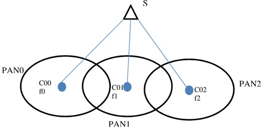
Figure 18. Network Organization ... 68

Figure 19. Proposed network topology ... 68

Figure 20. Changing cell procedure ... 74

Figure 21. A multi-road network ... 76

Figure 22. Single road use case for different LQIthreshold ... 79

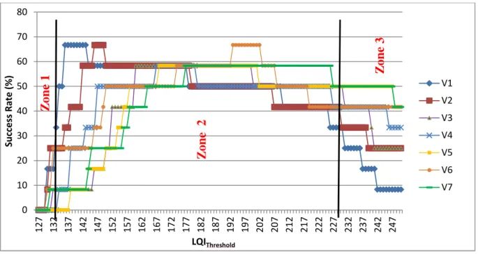
Figure 23. Success rate vs. LQIthreshold and speed ... 79

Figure 24. Success rate vs. LQIthreshold and speed ... 80

Figure 25. Energy gain for the Single-road and the Multi-road use cases in comparison to the standard ... 82

Figure 26. Energy gain for the Single-road and the Multi-road use cases in comparison to the standard ... 82

Figure 27. LQI value during node movement through a cell ... 83

Figure 28. Coordinators in the grid architecture ... 85

Figure 29. Energy spent in cell reselection procedures for different β values ... 86

(13)

Page (ii)

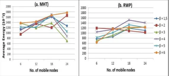
Figure 31. Average energy and average dalay during cell reselection procedures ... 89

Figure 32. Gain in average energy and average delay using 3 different mobility models ... 90

Figure 33. Average energy spent in cell reselection procedures (MHT model) ... 91

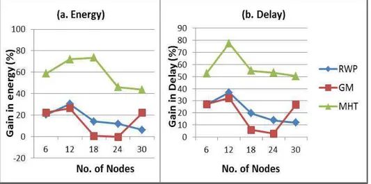
Figure 34. Gain in energy (MHT model) ... 91

Figure 35. Gain in delay (MHT model) ... 92

Figure 36. Remaining energy of node M vs. number of end devices ... 93

Figure 37. Number of received beacons by node M vs. Number of end devices... 93

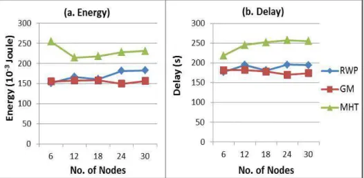
Figure 38. Average energy and average delay during cell reselection procedures ... 95

Figure 39. Gain in average energy and average delay using 3 different mobility models ... 95

Figure 40. Grid architecture ... 97

Figure 41. Gain in energy of the probabilistic speculative algorithm in comparison with same-road algorithm ... 99

Figure 42. Gain in delay of the probabilistic speculative algorithm in comparison with same-road algorithm ... 99

Figure 43. Average number of received beacons ... 105

Figure 44. Average remaining energy ... 105

Figure 45. Number of received beacons for communicating nodes ... 107

Figure 46. Remaining energy of communicating nodes ... 107

Figure 47. Packet delivery ratio ... 107

Figure 48. Remaining energy of communicating nodes Vs. CBR interval ... 108

Figure 49. Number of received beacon of communicating nodes Vs. CBR interval ... 109

Figure 50. Packet delivery ratio of communicating nodes Vs. CBR interval ... 109

Figure 51. Data rate adaptation during packet exchange ... 113

Figure 52. State machine of the unslotted CSMA-CA algorithm in WSNet simulator... 120

Figure 53. Modified state machine of the unslotted CSMA-CA algorithm in WSNet ... 121

Figure 54. Packet delivery ratio (PDR) at the MAC sublayer vs. network nodes’ number for static (Stc) and mobile (Mob) scenarios ... 122

Figure 55. CBR Packet delivery ratio (PDR) vs. network nodes’ number for static (Stc) and mobile (Mob) scenarios ... 122

Figure 56. Energy consumption in both scenarios vs. network nodes’ number for static (Stc) and mobile (Mob) scenarios ... 123

Figure 57. Gain in energy in comparison to the standard for static (Stc) and mobile (Mob) scenarios ... 123

(14)

Page (iii)

(15)

Page (i)

List of Tables

Table 1. Overview of short range protocols [Lee 2007] ... 4

Table 2. A Comparison of WSN technologies [Cao 2009] ... 6

Table 3. Frequency band of the IEEE 802.15.4 ... 16

Table 4 Topologies characteristics ... 51

Table 5. Overview of link quality estimators ... 60

Table 6 Available rates... 61

Table 7. Network simulators ... 70

Table 8 CC2420 energy consumption values [CC2420] ... 72

Table 9 Common simulation setup for the mobility management approach ... 72

Table 10 Energy consumption Evaluation of the standard procedure ... 72

Table 11 Simulation setup ... 88

Table 12. Simulation setup for noisy environment... 94

Table 13. Zones of a coordinator ... 97

Table 14. Rotation Table to determine the next zone ... 98

Table 15. Coordinates of the next coordinator ... 98

Table 16. Simulation setup in mobility-aware rate adaptation algorithm evaluation ... 104

Table 17. Simulation setup for the adaptive data rate adaptation algorithm ... 117

(16)

Page (1)

Chapter 1. Introduction

1.1. General context

Energy consumption resulting in global CO2 emission and battery waste caused by data communication and networking devices is increasing exponentially. Information and communication technology (ICT) is responsible for about two percent of the global CO2 emissions. However, ICT includes Internet of things (IoT) technologies and applications that have a direct effect on lowering CO2 emissions by increasing energy efficiency, reducing power consumption, and achieving efficient waste recycling. IoT has, therefore, an interesting dual role in CO2 emission [CarbonRoom] [Vermesan 2011] since its developments show that we will have 16 billion connected devices by the year 2020 (i.e. average out to six devices per person on earth and to many more per person in digital societies) [Vermesan 2011]. A recent report by the Carbon War Room [CarbonRoom] estimates that the incorporation of machine-to-machine communication in the energy, transportation, and agriculture sectors could reduce global greenhouse gas emissions by 9.1 gigatons of CO2 equivalent annually. Nowadays there is a need to develop applications that are environmentally friendly. In this context, the GRECO project (GREen wireless Communicating Objects) proposed to study the design of autonomous communicating objects. This means that, within a given time period, the power consumption is lower than or equivalent to the energy the object can harvest from its environment. The approach developed in GRECO aims at reaching a global power optimization for a communicating object.

This thesis is conducted as part of the GRECO project and as a joint guardianship with the National Engineering School of Sfax (Tunisia) and the LEAT from the University of Nice Sophia Antipolis. In this context, I conceived a new mobility management approach for mobile IEEE 802.15.4/ZigBee end device. The new approach reduces the energy consumption of the devices and it also increases their synchronization time.

(17)

Page (2)

During a semester internship in the computer science engineering department of the Hong Kong University of Science and Technology, I have focused on the rate adaptation feature for IEEE 802.15.4 protocol. An efficient rate adaptation algorithm has been proposed. Then a joint rate adaptation and mobility management approach have been conceived.

In the next subsection, we will introduce and compare the main short range wireless protocols.

1.2. Short range protocols

Wireless protocols were first proposed to replace wires that were not suitable to all environments. They progressively gained a bigger place in the market mainly thanks to the diversity of their use and the easiness of their deployment. The diversity of applications offered by wireless protocols led to the emergence of new protocol standards, each one is usually dedicated to a specific use and thus, it better fits some applications among others. Nowadays, one of the most challenging constraints in wireless communication is the energy consumption. This constraint is even more important in the personal area networks (PAN) given that PAN nodes have to operate autonomously over a long period of time (e.g. order of years for wireless sensors). Reducing the energy consumption can affect the communication

range. In fact, the higher the range, the higher the signal power; and thus, the higher the

energy consumption is.

Four main protocol standards for short range wireless communication with low energy consumption have recently gained a big interest in research: Bluetooth (over IEEE 802.15.1), ultra-wideband (UWB, over IEEE 802.15.3), ZigBee (over IEEE 802.15.4) [IEEE TG 15.4 2006] [ZigBee], and Wi-Fi (over IEEE 802.11). In [Lee 2007], a comparative study of short range communication protocols was proposed. The comparison was based on many criteria such as the radio channels, the network size, the maximum signal rate and the basic cell architecture. Table 1 summarizes the different characteristics of each protocol: the frequency band, the modulation technique, the maximum signal rate, the basic cell architecture, the complex structures that can be built from the basic cell, etc. Bluetooth, ZigBee and Wi-Fi protocols have spread spectrum techniques in the 2.4 GHz band, which is unlicensed in most countries and known as the industrial, scientific, and medical (ISM) band. Protocols use the spread spectrum technique indoors to be more resistant to interferences and noise. Bluetooth uses frequency hopping (FHSS) with 79 channels and 1 MHz bandwidth. ZigBee uses direct sequence spread spectrum (DSSS) with 16 channels and a maximum bandwidth of 2 MHz.

(18)

Page (3)

Wi-Fi uses DSSS (802.11), complementary code keying (CCK, 802.1lb) or OFDM modulation (802.1 1a/g) with 14 RF channels (11 available in US, 13 in Europe, and just 1 in Japan) and 22 MHz bandwidth. UWB uses the 3.1-10.6 GHz band, with an unapproved and jammed 802.15.3a standard, in which two spreading techniques are available: direct sequence-UWB (DS-UWB) and multi-band orthogonal frequency division multiplexing (MB-OFDM). The range of IEEE 802.15.4 can reach 100 meters. It is longer than Bluetooth (10 meters), but less than WLAN technologies.

It is important to point out that thanks to the robustness of the physical layer, the range of IEEE 802.15.4 transceiver is comparable to that of a IEEE 802.11 transceiver, but with a lower transmission power: from Figure 1 we can see that at an equal level of signal to noise ratio (SNR), 802.15.4 has a better BER compared to other wireless technologies.

Figure 1. ZigBee robustness [Freescale]

Bluetooth considered a new protocol dedicated to energy-constrained systems: Bluetooth Smart (low energy) (BLE). However, BLE constitutes a single-hop solution applicable to a different space of use cases in areas such as healthcare, consumer electronics, smart energy and security [Gomez 2012]. Besides, a BLE device used for continuous data transfer would

(19)

Page (4)

not have lower power consumption than a comparable Bluetooth device transmitting the same amount of data. It would likely use more power, since the protocol is dedicated to applications that need to transmit data over short communication burst before quickly tearing down the connection. Thus, BLE is only optimized for small bursts [Bluetooth].

Table 1. Overview of short range protocols [Lee 2007]

Standard Bluetooth UWB ZigBee Wi-Fi

IEEE spec. 802.15.1 802.15.3a 802.15.4 802.11a/b/g Frequency band 2.4 Ghz 3.1-10.6 Ghz 868/915 Mhz ;

2.4 Ghz 2.4 Ghz ; 5Ghz Max signal rate 1 Mb/s 110 Mb/s 250 kb/s 54 Mb/s

Nominal range 10 m 10 m 10 - 100 m 100 m Nominal TX power 0 - 10 dBm -41.3 dBm/MHz (-25) - 0 dBm 15 – 20 dBm Number of RF channels 79 (1 – 15) 1/10 ; 16 14 (2.4 GHz) Channel bandwidth 1 MHz 500 MHz – 7.5 GHz 0.3/0.6 MHz ; 2 MHz 22 MHz Modulation type GFSK BPSK, QPSK BPSK( +ASK), O-QPSK BPSK, QPSK, COFDM, CCK, M-QAM Spreading FHSS DS-UWB, MB-OFDM DSSS DSSS, CCK, OFDM Coexistence mechanism Adaptive freq. hopping Adaptive freq. hopping Adaptive freq. hopping Dynamic freq. Selection; Transmit power control (802.11h)

Basic cell Piconet Piconet Star BSS

Extension of the basic

cell Scatternet Peer-to-peer

Cluster tree,

Mesh ESS

Max number of cell

nodes 8 8 65536 2007

As it has been mentioned earlier, each protocol is more suitable depending on the application targeted. For instance, Bluetooth is used to connect cordless peripheral such as mouse, keyboard, and hands-free headset. UWB is oriented to multimedia applications requiring high-bandwidth. ZigBee is designed for reliable wirelessly networked monitoring and control networks. Wi-Fi is directed at computer-to-computer connections as an extension or substitution of cabled networks [Lee 2007].

(20)

Page (5)

1.1. Wireless Sensor Networks

Wireless sensor networks (WSN) are dedicated to short range wireless communications with low energy consumption. They are designed to handle a small amount of transmitted data generally corresponding to battery-operated sensors measurements (e.g. temperature, pressure, security cameras, controllers for water sprinklers, etc.). They have limited memory and computational capacity. Their use has become widespread in industrial environment, in home automation systems and in military systems [Garcia 2007]. Standardized protocols and proprietary protocols have been proposed. Based on the comparison given in Table 1, the ZigBee protocol has proved to be simpler than the Bluetooth, UWB, and Wi-Fi, which makes it very suitable for sensor networking applications. Other proprietary protocols have been used in sensor networks. However, for the sake of the interoperability between devices, a standardized protocol is preferable. Table 2 was given in [Cao 2009] and it compares some of these proprietary technologies (the Z-wave, Insteon, ANT, etc.) in addition to the ZigBee protocol based on the most common parameters such as the frequency band, the data rate, the corresponding network topology. Almost all protocols use the 2.4 GHz ISM band. This common characteristic can be considered as a first level of standardization. Therefore, it should also be mentioned that even a proprietary protocol has to be in compliance with a number of rules and meet some compatibility requirements such as the national authorities’ regulation for radio transmission.

As it is detailed in subsection 1.2, many constraints are considered when designing and deploying sensor networks. The main constraints are related to the energy consumption, the production cost, the hardware limitation, the operating environment, the network topology, the range, the transmission medium and the throughput. This is the reason that makes compromises in term of data rate essential. Depending on the application, additional constraints are added such as mobility management, energy management, etc. Some of these constraints (low consumption, high throughput and large range) are so contradictory that it will never be a unique standard since different solutions can be considered. This gives space to researchers to propose different approaches. Low consumption, high throughput and large range are important factors and are usually used as guidelines to develop algorithms and protocols used in sensor networks. They are also considered as metrics for comparing performance between different solutions in this field.

(21)

Page (6)

Table 2. A Comparison of WSN technologies [Cao 2009]

Technology Frequency band Data rate (b/s) Multiple access method Coverage area (meter) Network topology Bluetooth Low

Energy 2.4 GHz ISM 1 M FH + TDMA 10 Star

UWB

( ECMA – 368)

3.1 – 10.6

GHz 480 M CSMA/ TDMA <10 Star

Bluetooth 3.0 +

High Speed 2.4 GHz ISM 3 – 24 M

FH +

TDMA/CSMA (WiFi)

10 Star

ZigBee

(IEEE 802.15.4) ISM 250 K CSMA 30-100

Star/ mesh Insteon 131.65 KHz (powerline) 902 – 924 MHz

13 K Unknown Home area Mesh

Z- wave 900 MHz

ISM 9.6 K Unknown 30 Mesh

ANT 2.4 GHz ISM 1 M TDMA Local area Star/

mesh RuBee (IEEE 1902.1) 131 KHz 9.6 K Unknown 30 Peer-to-peer RFID (ISO/IEC 18000-6) 860-960 MHz 10-100 K Slotted- Aloha/ binary tree 1-100 Peer-to-peer FH: Frequency hopping

TDMA: Time division multiple access CSMA: Carrier sense multiple access

1.2. Challenges in WSN

Communication between sensor nodes faces more challenges than communication in other wireless networks. The constraints imposed by sensor architecture makes it hard to ensure a high quality of service (QoS). Besides, the low signal power used to transmit data makes the signal very vulnerable to channel disturbance. The main challenges to which sensor networks are confronted are mainly the low energy budget, the channel conditions, the collisions that may occur during the packet transmission and the mobility which has to be ensured in many WSN applications. All these features are detailed below.

1.2.1. Energy consumption

Each single execution within electronic devices needs energy. This is why energy consumption optimization is a matter raised at every level from the sensor architecture design

(22)

Page (7)

phase to the phase of WSN protocol applications’ conception. Besides, WSN nodes are supposed to work autonomously for a long period of time, a low energy budget will impose in certain cases adjustments in the system functionalities in order to reduce the energy consumption [Shah 2002]. The energy budget is, then, both an evaluation metric that gives information about some algorithms performance and a decision metric used by protocol algorithms.

The transmission unit consumes the biggest part of the energy [Raghunathan 2002]. Indeed, datasheets of commercial sensor nodes show that the energy cost of receiving or transmitting a single bit of information is approximately the same as that required by the processing unit for executing a thousand operations [Crossbow] [Tmote]. To overcome this shortcoming, the sleep and the idle modes are used in sensor nodes. In the sleep mode, significant parts of the transceiver are switched off. The node is not able to immediately receive data and needs a recovery time to leave the sleep state (energy consumed during the startup can be significant). In the idle mode, the node is ready to receive, but it is not doing so. Some functions in the hardware can be switched off, thus, reducing the energy consumption. The use of sleep and idle modes raises a new problem which is the synchronization of network nodes. Devices need to know when to switch between the different states: receive, transmit, idle and sleep modes. Moreover, a clock drift may occur [Ganeriwal 2005]. In this case, control packets have to be transmitted to resynchronize the network, which increases the energy consumption. The major goal when designing WSN applications is to ensure the optimal throughput with a low energy budget according to the targeted application requirements [Chandrakasan 1999].

1.2.2. Channel conditions

Signal distortion during the packet transmission can be caused by predictable and quantifiable phenomena (at least when the transmission environment is well known) and by unpredictable events. The main predictable phenomena are the propagation which consists in the attenuation of the transmitted signals with the distance (path loss), the blocking of signals caused by large obstacles (shadowing), and the reception of multiple copies of the same transmitted signal (multipath fading). These variations can be roughly divided into two types [Tse 2005]:

• Large-scale fading, due to path loss of signal as a function of distance and shadowing by large objects such as buildings and hills. This occurs as the mobile moves through a

(23)

Page (8)

distance of the order of the cell size (cellular system), and is typically frequency independent.

• Small-scale fading, due to the constructive and the destructive interference of the multiple signal paths (multipath fading) between the transmitter and receiver. This occurs at the spatial scale of the order of the carrier wavelength, and it is frequency dependent.

Large-scale fading is more relevant to issues such as cell-site planning. Small-scale multipath fading is more relevant to the design of reliable and efficient communication systems.

Unpredictable events happen randomly and are completely unknown by the device. The corresponding effects are the thermal noise and interferences. The thermal noise is introduced by the receiver electronics and is usually modeled as Additive White Gaussian Noise (AWGN). If the medium is not shared with any other RF sources, the signal propagation of simulated transmitters and AWGN can describe the entire channel. However, when several nodes transmit at the same time on the channel, interferences may happen and have to be taken into account in the channel modeling.

In WSN, the transmission power is relatively low, which makes the signal very sensitive to noise. In addition, since the antennas used by the nodes are very close to the ground, the loss of the signal transmitted between them can be very high.

In [Tse 2005], it was highlighted that interference I from neighboring cell is random due to two reasons. One of them is small-scale fading and the other is the physical location of the user in the other cell that is reusing the same channel. The mean of I represents the average interference caused, averaged over all locations from which it could originate and the channel variations. However, due to the fact that the interfering user can be at a wide range of locations, the variance of I is quite high. Therefore, it was noticed in [Tse 2005] that the signal to interference plus noise ratio (SINR) is a random parameter leading to an undesirably poor performance. There is an appreciably high probability of unreliable transmission of even a small and fixed data rate in the frame.

In this work, we only focus on orthogonal interferences: Only interferences that happen in the same channel are considered.

(24)

Page (9)

1.2.3. Medium access

WSN have to handle the interconnection between a large number of devices. These devices usually use the same frequency (especially in Ad Hoc networks) to communicate. As a consequence, collisions may occur very often. Bad channel conditions may cause either delay and trigger a backoff period before sending data or the failure of the packet reception. Low network performance that is caused by the medium access mode is, therefore, closely related to the channel conditions and the physical layer design [Miluzzo 2008]. It is also interesting to mention that, given the large scale of sensor networks, the randomness of transmission time makes it difficult to analytically evaluate protocol performance. This is why simulation is an interesting alternative to study and evaluate sensor network protocols.

1.2.4. Mobility

The most important feature in the mobility management is maintaining the synchronization of mobile nodes. When nodes move, the routes of transmitted packets may change. The route change must be quickly handled in order to avoid high transmission delays. Even if the routing protocol differs from a network configuration to another [Norouzi 2012], route discovery always requires additional network overhead (control packets). In addition to delay increase, the packet reception rate may decrease because of the synchronization loss.

One of the direct effects of mobility during the transmission is the Doppler effect that occurs when the source and the receiver are in motion relative to each other. The wave frequency increases when the source and receiver approach each other and decreases when they move apart. The motion of the source causes a real shift in frequency of the wave, while the motion of the receiver produces only an apparent shift in frequency. The computation limitations of sensor nodes do not make the use of complex mobility management techniques possible.

1.3. Contributions and manuscript organization

This thesis proposes new approaches to handle self-efficient embedded system for mobile communicating objects. Therefore, we first examine the energy efficiency in IEEE 802.15.4 sensor networks based on the protocol standard and previous research. Our major concern is reducing the energy consumption of mobile sensor nodes. To do so, we proceed in two phases. At the first stage, we propose a global sensor network architecture and a new energy-efficient mobility management approach for IEEE 802.15.4/ZigBee end devices. The new approach is

(25)

Page (10)

based on the link quality estimator (LQI) and uses a speculative algorithm. We propose two speculative algorithms. Then, we study and evaluate the energy efficiency when using a rate adaptation algorithm that takes into account the channel conditions. We first propose a mobility-aware rate adaptation algorithm and evaluate its efficiency in our network architecture. Then, we propose and evaluate a second rate adaptation algorithm that relies on a more accurate link channel estimation.

This manuscript is organized as follows. In Chapter 2, we present an overview of the IEEE 802.15.4/ZigBee protocol. Chapter 3 is dedicated to the state of the art related to our work. In Chapter 4, the network architecture and the new mobility management approach as well as its evaluation are given. In Chapter 5, two rate adaptation algorithms are presented and evaluated. The conclusion and perspectives are given in Chapter 6.

(26)

Page (11)

Chapter 2. IEEE802.15.4/ZigBee

overview

2.1. Introduction

ZigBee is a high-level protocol for wireless personal area networks (WPANs) based on the IEEE 802.15.4 standard. As it is shown in Figure 1, IEEE 802.15.4 defines both the data link and the physical layers, respectively called the MAC and PHY layers in the following. ZigBee takes full advantage of the IEEE 802.15.4 specification, and adds the network, security, and application layers.

Figure 2. IEEE 802.15.4/ZigBee layers

This section introduces the generic sensor node architecture; then it offers an overview of

IEEE802.15.4/ZigBee layers. Finally, it details the energy consumption performance of the IEEE 802.15.4 physical and MAC layers and the ZigBee network layer.

PHY MAC Network/Security Application Framework ZigBee IEEE 802.15.4

(27)

Page (12)

2.2. Sensor node architecture

Sensor nodes are built with respect to some constraints [Bharathidasan 2002] [Raghunathan 2002]. In fact, the sensor nodes have to:

• be small (size)

• consume minimum energy

• operate in a high density (large concentration of operating nodes) • have a reduced production cost

• be independent and able to operate unattended • be adaptive to the environment

Figure 3. System architecture of a typical wireless sensor node [Bharathidasan 2002]

These constraints concern both the software and the hardware. The software part is handled by the communication protocol stack deployed within the sensor device. It is also constrained by the hardware architecture. In this section, the general hardware architecture of sensor devices is detailed. As it is illustrated in Figure 3, a sensor node contains four basic components listed below.

2.2.1. The sensing unit

The sensing unit typically includes two sub-units, the sensor itself in addition to an analog-to-digital converter (ADC) that converts analog signals produced by the sensors according to the observed phenomenon to digital signals that are transmitted to the processing unit.

(28)

Page (13)

2.2.2. The processing unit

The processing unit, usually associated with a small storage unit (memory), carries out the procedures that allow a node to work with the other nodes of the network to give, in the end, the result of the task assigned to the network.

2.2.3. The transmission unit

Connecting the node to the network is managed by the transmission unit. Communications are based on radio frequency-based components that require circuits of modulation, demodulation, filtering, and multiplexing, which increases the complexity of sensor nodes and their production cost. The realization and the use of components of radio transmission in sensor networks low energy consumption is so far a major technical challenge.

2.2.4. The power supply unit

The power supply unit is also one of the most important components in a sensor node. It can be represented by an energy charging system such as solar cells. The sensors are usually battery-powered. Their autonomy is acceptable for applications requiring the transfer of small amounts of data (their original applications). However, when the amount of exchanged data increases, autonomy decreases.

A sensor node may also contain a unit of power management (MM) that controls and adjusts its functions according to the energy budget.

2.3. IEEE 802.15.4 overview

2.3.1. IEEE 802.15.4 versions

Many revisions have been done to the IEEE 802.15.4 standard since its first appearance in 2003. The 2003 version defined two PHYs operating in different frequency bands (one for 868/915 MHz band and one for 2.4 GHz band) with a very simple, but effective, MAC layer protocol. In 2006, a new standard revision [IEEE TG 15.4 2006] added two more PHY options. These optional PHYs proposed a higher rate to the 868/915 MHz frequency bands. It added four modulation schemes that could be used: three for the lower frequency bands and

(29)

Page (14)

one for 2.4 GHz frequency band. The MAC was backward-compatible, but it added MAC frames with a variety of enhancements including:

• Support for a shared time base with a data time stamping mechanism • Support for beacon scheduling

• Synchronization of broadcast messages in beacon-enabled PANs

In 2007, two new PHYs, one for UWB technology and another one used for the Chirp Spread Spectrum (CSS) at 2.4 GHz frequency band, were added as an amendment.

In 2009, two new PHY amendments were approved, one to provide operation in frequency bands specific in China and the other for operation in frequency bands specific to Japan. The major changes in the current revision (2011) are not technical but editorial. The organization of the standard was changed so that each PHY now has a separate clause. The MAC clause was split into functional description, interface specification, and security specification.

2.3.2. IEEE 802.15.4 nodes

IEEE 802.15.4 defines two types of nodes:

• FFD (Full Function Device): these devices implement the whole protocol stack and can handle packet routing mechanism.

• RFD (Reduced Function Device): RFD node does not have the ability of routing packets. It does not implement the entire protocol stack.

2.3.3. IEEE 802.15.4 topology 2.3.3.1. Star topology

When FFD is activated for the first time, it can establish its own network and become the PAN coordinator. Star networks operate independently from all other star networks. This is possible if a PAN ID that is not used by another network being in the coverage area is chosen.

2.3.3.2. Point-to-point topology

In point to point topology (peer-to-peer), an FFD can communicate directly with other FFD provided they are within radio range of each other. In this topology, there is a single

(30)

Page (15)

coordinator as in star topology. Its role is to maintain a list of participants in the network and distribute short addresses.

2.3.3.3. More complex topologies

With the help of a network layer and a data packets routing system, it is possible to develop more complex topologies. ZigBee technology provides a network layer to easily create such topologies with automatic routing algorithms such as cluster tree (tree cells) or mesh networks. The advantage of a cluster tree is the possibility of extending the coverage area of the network, while its disadvantage is the increased latency.

2.3.4. Physical layer

The IEEE 802.15.4 protocol uses the ISM frequency band defined at the following frequencies:

• 2.4 GHz ISM band has 16 channels that are spaced 5 MHz apart with a spectral window of 2 MHz.

• 915 MHz (for USA) has 10 channels that are spaced 2 MHz apart with a spectral window of 0.6 MHz.

• 868 MHz (for Europe) has one channel with a spectral window of 0.3 MHz. The standard specifies the following four PHY layers:

• An 868/915 MHz direct sequence spread spectrum (DSSS) PHY employing binary phase-shift keying (BPSK) modulation.

• A 2450 MHz DSSS PHY. The modulation format is Offset – Quadrature Phase Shift Keying (O-QPSK) with half-sine chip shaping. This is equivalent to MSK modulation. Each chip is shaped as a half-sine, transmitted alternately in the I and Q channels with one half chip period offset.

In addition to the 868/915 MHz BPSK PHY, which was originally specified in the 2003 edition of this standard, two optional high-data-rate PHYs are specified for the 868/915 MHz bands, offering a tradeoff between complexity and data rate.

• An 868/915 MHz DSSS PHY employing offset quadrature phase-shift keying (O-QPSK) modulation

(31)

Page (16)

• An 868/915 MHz parallel sequence spread spectrum (PSSS) PHY employing BPSK and amplitude shift keying (ASK) modulation

The O-QPSK and the ASK PHYs are not mandatory in the 868 MHz or 915 MHz band. If one of them is used by a device in the 868 MHz or 915 MHz band, then the same device shall be capable of transmitting using the BPSK PHY as well.

The data rate of the 2.4 GHz O-QPSK is 250 kb/s. The BPSK PHY is 20 kb/s when operating in the 868/950 MHz band and 40 kb/s when operating in the 915 MHz band.

Table 3 summarizes the main characteristics (frequency, rate, number of channels) of the mandatory IEEE 802.15.4 PHY layers.

Table 3. Frequency band of the IEEE 802.15.4

PHY (MHz) Frequency Band Rate (kb/s) Number of channels Central frequency (MHz) 868/915 868-868.6 20 1 868.3 902-928 40 10 906+2(k-1) ; k=1,2,..,10 2450 2400-2483.5 250 16 2405+5(k-11) ; k=11,..,26

We are interested in the 2006 standard version and more specifically the IEEE 802.15.4 2.4 GHz frequency band. We consider that the specification is sufficient enough to study the protocol behavior in WSN.

2.3.4.1. O-QPSK 2.4 GHz PHY

The maximum power emitted by an IEEE 802.15.4 or ZigBee module is not defined by the standard. It depends on the regulatory authority of the area where the transmission is performed, and on the manufacturer according to the application that the node is meant to. However, the typical recommended power is 1 mW or 0 dBm and receiver sensitivity must be better than - 85 dBm at 2.4 GHz (for packet error rate less than 1%).

(32)

Page (17)

Figure 4. Modulation and spreading functions for the O-QPSK PHYs

DSSS multiplies the data stream with a high-data rate sequence called chip sequence or Pseudo-Noise (PN) sequence. Therefore, the resulting signal determined by the pseudo-random signal can occupy larger bandwidth. Due to its length, the PN sequence seems as a random signal, like noise. However, it is a completely deterministic signal, which enables the reconstruction of the original data stream on the receiver side. The reconstitution is possible even if the signal is distorted during the transfer and the original sequence can still be extracted from the transmission due to its redundancy in the carrying signal. Thus, DSSS istolerant to noise and has the advantage of making the signals of a limited bandwidth like a voice signal more resistant to noise during the transmission. However, spreading the transmit signal power within a larger bandwidth decrease the transmit power.

As it is illustrated in Figure 4, in 2.4 GHz O-QPSK PHY layer, each byte is divided into two symbols, four bits each (S0 and S1). Each symbol is mapped to one out of 16 pseudo-random sequences, 32 chips each. The chip sequences are modulated using O-QPSK. The rate of the 2.4 GHz band is 250 kb/s. The chip sequence is, then, transmitted at 2 MChips/s.

The BER is computed from the SINR and the modulation used. The SINR can be defined as follows:

= ∗ | | ⁄ + (1)

The numerator is the received power at the base-station due to the user transmission of interest with P denoting the average received power and |h|2 the fading channel gain (with

Bit-to-Symbol 1010 1001 bitstream 1010 1001 S1 S0 Sender Receive 0 31 O-QPSK Modulator Symbol-to-Chip 0 31 Chip-to-Symbol Symbol-to-Bit ≠? 1010 1001 S1 S0 1010 1001 bitstream Modulated Signal MSK De-Modulator

(33)

Page (18)

unit mean). The denominator consists of the background noise N0 and an extra term due to the

interference from the user in the neighboring cell. I denotes the interference and is modeled as a random variable with a mean typically smaller than P (say equal to 0.2P).

The bit error probability Pb for QPSK is the same as for BPSK.

= ∗ = (2)

! = _√# $*+ %&' ₍₎

, (3)

QPSK modulation consists of BPSK modulation on both the in-phase and quadrature components of the signal. With perfect phase and carrier recovery, the received signal components corresponding to each of these branches are orthogonal. Therefore, the bit error probability on each branch is the same as for BPSK: Pb = Q(Pb2). The symbol error

probability equals the probability of either branch has a bit error:

_- = 1 − 1 − ! (4)

The snr is related to the in that:

= 212 (5)

During the demodulation stage, the received signal is converted to binary codes. The conversion uses either soft decision decoder (SDD) or hard decision decoder (HDD). If the soft decision decoder is being used, the symbol is decoded and extra information about the most likelihood is determined and gives the probability of the correctness of the decoding. Let xk (k = 1 .. N) be the input bits to the encoder of the sender, r the received signal input to

the decoder of the receiver. The output of the decoder at the receiver is log likelihood ratio (LLR) for each received bit:

334 5! = log 9 ,:; |<)

9(,:;=|<)) (6)

The decoded output bit yk is determined as follows:

>? = @1 ∶ 334(5) ≥ 1_{0 ∶ 334(5) < 0} (7)

On the other hand, if HDD is being used, each symbol is determined independently of other symbols. HDD uses the Hamming Distance between the received word and the code word (the number of distinct elements between the two words). The SDD is more costly than the

(34)

Page (19)

HDD; however, it is more accurate. IEEE 802.15.4 devices usually use a Hard Decision

Decoder (HDD) (e.g. the IEEE 802.15.4-compliant ChipCon CC2420). 2.3.4.2. PHY layer services

The PHY layer is responsible for the following tasks:

• the activation and deactivation of the radio transceiver, • the energy detection (ED) task,

• Link quality indicator (LQI) for received packets, • Clear channel assessment (CCA),

• Channel frequency selection, • Data transmission and reception. i. Energy detection (ED)

The energy detection mechanism allows having an estimation of the received signal power within the bandwidth of the channel with no attempts to identify or decode the signal. The duration of the ED is equal to 8 symbols.

ii. Link quality indicator (LQI) for received packets

When a packet is received by a node, its link quality can then be determined. The IEEE 802.15.4 standard defines the link quality indicator (LQI) as an integer ranging from 0 to 255. However, the calculation of the LQI is not specified in the standard. The LQI measurement is a characterization of the strength and/or quality of a received packet. IEEE 802.15.4 specifies that the measurement may be implemented using receiver energy detection (ED), a signal-to-noise ratio estimation (SNR), or a combination of these methods. The use of the LQI metric by the network or application layers is not specified in the standard as well. Although the calculation of the LQI is not specified in the standard, its definition implies that it depends on the distance between the receiver and the sender.

iii. Clear channel assessment (CCA)

IEEE 802.15.4 nodes use the carrier sense multiple access with collision avoidance (CSMA-CA) mechanism to send packets. The CSMA-CA mechanism is a MAC mechanism (subsection 2.3.5) that consists of listening to the channel before sending packets. A node sends packets if the channel is sensed to be free. In order to do so, the CSMA-CA uses the

(35)

Page (20)

CCA PHY mechanism that allows an IEEE 802.15.4 node to listen to the channel during 8 symbols. There are 3 modes of CCA:

• Mode 1: Energy above threshold: the medium is busy if energy above the ED threshold is detected.

• Mode 2: Carrier sense only: the medium is considered busy if the node senses a signal compliant with the standard with the same modulation and spreading characteristics of the PHY that is currently in use by the device. This signal may be above or below the ED threshold.

• Mode 3: Carrier sense with energy above threshold: a combination between the two previous techniques.

iv. Channel frequency selection:

In the initialization of the network, the coordinator has to choose the appropriate frequency in order to avoid collisions between packets that are transmitted in the neighbor networks.

v. Data transmission and reception

The PHY handles the transmission and reception of physical layer protocol data units (PPDUs) across the physical radio channel. PPDU is the information received at the PHY layer and that is composed of control information (a synchronization header (SHR) and a PHY header (PHR) that contains the frame length information) and data (MAC protocol data unit: MPDU).

2.3.5. Mac sublayer

The MAC sublayer is mainly responsible for the synchronization of the network in order to optimize packet transmissions. This is ensured through the beacon management and several other mechanisms (e.g. association, dissociation, channel access, acknowledgment frame delivery, GTS management).

For the sake of simplicity, the MAC personal area network information base (PIB) attributes and MAC constants that are named in this section are given in Some MAC attributes and constants.

(36)

Page (21) 2.3.5.1. Beacon management

IEEE 802.15.4 wireless network has a coordinator which always initializes the network defined by an identifier. The coordinator is always an FFD device. There are two types of PANs: non beacon-enabled and beacon-enabled PAN. In beaconless mode, there is no synchronization between nodes. A node wishing to send a message on the channel must first listen on it. If it is free, message can be sent. Otherwise a node has to wait for an interval of time called backoff period and start again. This is handled according to the non-slotted version of the CSMA-CA protocol. The beacon mode is a synchronized mode. Access to the medium is done using the Time Division Multiple Access method (TDMA). The time is divided into superframes. In a non beacon-enabled mode, a node can ask for a beacon by sending a beacon request to the coordinator.

The beacon frame contains essential information about the channel that is used, the PAN identifier (PAN Id), as well as the PAN mode.

2.3.5.2. Superframe format

As shown in Figure 5, each superframe in the beacon-enabled mode consists of an active period in which nodes can receive and transmit and an optional inactive period during which all nodes enter into a low-power mode. The macBeaconOrder (BO) is a MAC PIB attribute that defines the beacon interval (BI). BI represents the entire period between two consecutive beacon frames and it is defined as follows:

EF = GEG1 HIJ GK LI G)MN2 ∗ 2OP ₍₈₎

where 0 <= BO <= 14 and aBaseSuperframeDuration is a MAC constant that represents the minimum duration of a superframe. aBaseSuperframeDuration is fixed to 960 symbols. The macSuperframeOrder (SO) is a MAC attribute that defines the duration of the active period called superframe duration (SD). It is defined as follows:

HF = GEG1 HIJ GK LI G)MN2 ∗ 2QP ₍₉₎

where 0 <= SO <= BO <= 14 .

The active period is composed of 16 slots (Figure 5). Each beacon interval begins with the synchronization beacon message sent by the coordinator to all nodes of the network. The remaining 15 slots are divided into a contention access period (CAP) and an optional contention free period (CFP). In CAP, the channel is accessed according to the slotted version

(37)

Page (22)

of the CSMA / CA protocol. In CFP, the coordinator assigns guaranteed time slots (GTS) that are composed of one or more slots. A node may request GTS assignment from the coordinator during the CAP period.

Figure 5. IEEE 802.15.4 Beacon-enabled Superframe

In the beacon-enabled mode, if macSuperframeOrder (SO) is set to 15, the superframe does not remain active after the beacon.

In the non beacon-enabled mode, the macBeaconOrder (BO) is set to 15 and the

macSuperframeOrder (SO) value is ignored. In this mode, the coordinator transmits beacon

frames only when it is requested to do so, such as on receipt of a beacon request command. 2.3.5.3. Channel access

Depending on the type of the PAN that is defined (beacon-enabled or non beacon-enabled PAN), the channel access is ensured by the CSMA-CA algorithm or by the GTS mode. The standard defines two channel access modes at the media access control sub layer (MAC): the unslotted mode and the slotted mode. If periodic beacons are not being used in the PAN or if a beacon could not be located in a beacon-enabled PAN, the MAC sublayer transmits using the unslotted version of the CSMA-CA algorithm.

0 ₁ 2 3 4 5 6 7 8 9 A B C D E F Active Period Inactive Period CFP (GTS) CAP (CSMA-CA) beacon _t Superframe

(38)

Page (23) i. GTS mode:

Figure 6. GTS and Backoff slots in IEEE 802.15.4 Beacon-enabled Superframe

A maximum total number of 7 GTSs can be allocated in 1 superframe. A GTS is a portion of the superframe exclusively dedicated to one node so it can transmit or receive packets without collision risks. This can be ensured thanks to the broadcasting of the information about the allocated GTSs and the length of the CAP period in the beacon. The length of an allocated GTS is not limited and the start of the GTS slot has no constraint. However, as it is illustrated in Figure 6, the communication within a GTS must end one interframe-spacing (IFS) (subsection 2.3.5.4) before the actual GTS is ended. A node sends GTS requests to its coordinator in the CAP period using the slotted CSMA-CA mode specifying the number of slots requested and the direction of the transmission (receive or transmit). A data frame transmitted in an allocated GTS uses only short addressing (see 2.4.2). If a device (coordinator or another device) has been allocated a receive GTS, its receiver has to be on during the entire period of the GTS.

On the receipt of a GTS allocation request frame, the PAN coordinator first checks if there is available capacity in the current superframe, based on the remaining length of the CAP and

IFS IFS (2.3.5.4) CFP (GTS) CAP (CSMA-CA) 0 ₁ 2 3 4 5 6 7 8 9 A B C D E F Active Period Inactive Period beacon _t GTS Pslot Packet n Packet n+1

(39)

Page (24)

the desired length of the requested GTS. When the PAN coordinator determines whether capacity is available for the requested GTS, it generates a GTS descriptor with the requested specifications and the 16-bit short address of the requesting device. The GTS descriptor is sent to the requesting node in the beacon frame. GTSs are allocated on a first-come-first-served basis by the PAN coordinator provided there is sufficient bandwidth available. Each GTS descriptor is 24 bits in length and contains the following information:

• The device short address is 16 bits in length of the device for which the GTS descriptor is intended

• The superframe slot (4 bits in length) at which the GTS is to begin.

• The number of contiguous superframe slots over which the GTS is active (4 bits in length).

If a device misses the beacon at the beginning of a superframe, it cannot use its GTSs until it receives a beacon correctly. There is no limit on the GTS use. The GTS is deallocated either on the node request or on PAN coordinator decision (usually because of node’s inactivity during a determined number of superframes).

ii. CSMA-CA Algorithm ( Annex A)

The CSMA-CA algorithm allows network nodes to share the same channel. It provides a channel access mechanism that avoids collisions between different transmitted signals by listening to the medium before starting to transmit. The transmission is deferred if the channel is found to be busy (used by another transmitting source). This mechanism considerably reduces collision probability. However, collisions still can happen unlike when transmitting during a GTS. Nonetheless, the CSMA-CA mechanism is essential even for the GTS transmission mode since the GTS requests (and all other control frames) have to be sent during the CAP period. Moreover, the GTS mechanism is hard to be achieved in real applications because of the synchronization issue and the risk of clock drift.

CSMA-CA is based on the backoff period unit. The CAP is not considered as a sequence of

slots as in the CFP; it is considered as a sequence of backoff slots that have aUnitBackoffPeriod period. In slotted CSMA-CA, the start of the first backoff period of each

device is aligned with the start of the beacon transmission. In unslotted CSMA-CA, the backoff periods of one device are not related in time to the backoff periods of any other device in the PAN.

(40)

Page (25)

Figure 7 describes the CSMA-CA mechanism in the slotted mode. According to the related algorithm, two consecutive CCAs are required before the transmission can start. In Figure 7, the time required for each CCA is denoted TCCA. CCA is performed at the beginning of a

backoff period (TBP in Figure 7). The contention window (CW) variable controls the number

of CCAs to be performed in each attempt. CW is, therefore, initialized to two and reset each time the channel is assessed to be busy. If the channel is busy, the node has to wait for a computed number of backoff periods. The number of backoff is constrained by a second variable, NB, which is the number of times the CSMA-CA algorithm was required to backoff while attempting the current transmission. This value is initialized to zero before each new packet transmission. Each time a current transmission attempt fails, NB is incremented.

Figure 7. CSMA-CA Algorithm in the slotted mode TBeacon Active Period T CCA TCCA T_IFS CCA IFS IFS CFP (GTS) CAP (CSMA-CA) 0 ₁ 2 3 4 5 6 7 8 9 A B C D E F Inactive Period beacon _t Pslot Packet Unsuccessful CCA C C A C C A TBP