HAL Id: hal-03103470
https://hal.archives-ouvertes.fr/hal-03103470
Submitted on 14 Jan 2021
HAL is a multi-disciplinary open access
archive for the deposit and dissemination of
sci-entific research documents, whether they are
pub-lished or not. The documents may come from
teaching and research institutions in France or
abroad, or from public or private research centers.
L’archive ouverte pluridisciplinaire HAL, est
destinée au dépôt et à la diffusion de documents
scientifiques de niveau recherche, publiés ou non,
émanant des établissements d’enseignement et de
recherche français ou étrangers, des laboratoires
publics ou privés.
Continuous measurements of atmospheric water vapour
isotopes in western Siberia (Kourovka)
V. Bastrikov, H. Steen-Larsen, V. Masson-Delmotte, K. Gribanov, O. Cattani,
J. Jouzel, V. Zakharov
To cite this version:
V. Bastrikov, H. Steen-Larsen, V. Masson-Delmotte, K. Gribanov, O. Cattani, et al.. Continuous
measurements of atmospheric water vapour isotopes in western Siberia (Kourovka). Atmospheric
Measurement Techniques, European Geosciences Union, 2014, 7 (6), pp.1763-1776.
�10.5194/AMT-7-1763-2014�. �hal-03103470�
Atmos. Meas. Tech., 7, 1763–1776, 2014 www.atmos-meas-tech.net/7/1763/2014/ doi:10.5194/amt-7-1763-2014
© Author(s) 2014. CC Attribution 3.0 License.
Continuous measurements of atmospheric water vapour isotopes in
western Siberia (Kourovka)
V. Bastrikov1,2,3, H. C. Steen-Larsen2, V. Masson-Delmotte2, K. Gribanov1, O. Cattani2, J. Jouzel2, and V. Zakharov1
1Ural Federal University, Ekaterinburg, 620002, Russia
2LSCE/IPSL, UMR8212, CEA-CNRS-UVSQ, CEA Saclay, Gif-sur-Yvette, 91191, France 3Institute of Industrial Ecology UB RAS, Ekaterinburg, 620219, Russia
Correspondence to: V. Bastrikov (v.bastrikov@gmail.com)
Received: 3 October 2013 – Published in Atmos. Meas. Tech. Discuss.: 21 January 2014 Revised: 23 April 2014 – Accepted: 7 May 2014 – Published: 18 June 2014
Abstract. The isotopic composition of atmospheric water
vapour at the land surface has been continuously moni-tored at the Kourovka astronomical observatory in western Siberia (57.037◦N, 59.547◦E; 300 m a.s.l.) since April 2012. These measurements provide the first record of δD, δ18O and d-excess in this region. Air was sampled at 8 m height within a forest clearing. Measurements were made with a wavelength-scanned cavity ring-down spectroscopy ana-lyzer (Picarro L2130-i). Specific improvements of the mea-surement system and calibration protocol have been made to ensure reliable measurements at low humidity during win-ter. The isotopic measurements conducted till August 2013 exhibit a clear seasonal cycle with maximum δD and δ18O values in summer and minimum values in winter. In addi-tion, considerable synoptic timescale variability of isotopic composition was observed with typical variations of 50– 100 ‰ for δD, 10–15 ‰ for δ18O and 2–8 ‰ for d-excess. The strong correlations between δD and local meteorologi-cal parameters (logarithm of humidity and temperature) are explored, with a lack of dependency in summer that points to the importance of continental recycling and local evapotran-spiration. The overall correlation between δD and tempera-ture is associated with a slope of 3 ‰◦C−1. Large d-excess diurnal variability was observed during summer with up to 30 ‰ decrease during the night and the minima manifested shortly after sunrise. Two dominant diurnal cycle patterns for d-excess differing by the magnitude of the d-excess decrease (21 ‰ and 7 ‰) and associated patterns for meteorological observations have been determined. The total uncertainty of the isotopic measurements was quantified as 1.4–11.2 ‰ for
δD, 0.23–1.84 ‰ for δ18O and 2.3–18.5 ‰ for d-excess de-pending on the humidity.
1 Introduction
The isotopic composition of atmospheric water vapour is a valuable source of information for quantifying the pro-cesses controlling the hydrological cycle. The saturation vapour pressures and air diffusivities of the natural stable iso-topologues of water, H216O, HD16O and H218O, are slightly different (Merlivat and Nief, 1967; Majoube, 1971; Merlivat, 1978; Barkan and Luz, 2007; Ellehoj et al., 2013). As a re-sult, fractionation takes place during each phase change such as evaporation from the sea surface (Craig and Gordon, 1965; Merlivat and Jouzel, 1979), soil evaporation and plant tran-spiration from land surface (Farquhar et al., 2007), conden-sation in the clouds (Jouzel, 1986; Ciais and Jouzel, 1994), and rain re-evaporation and diffusive exchange processes be-tween raindrop and vapour (Stewart, 1975; Field et al., 2010). This fractionation therefore leads to spatial and temporal variations in the isotopic composition of atmospheric water vapour and precipitation. Thus, stable isotopes of water can be exploited as natural tracers of atmospheric transport pat-terns and physical processes involving water vapour in the atmosphere.
For the last several decades water isotope measurements have focused on liquid water (precipitation, surface water, soil moisture, groundwater, etc.) as a means to investigate the hydrological cycle processes (Dansgaard, 1964; Rozanski et al., 1993; Gat, 1996). Fewer measurements of atmospheric water vapour have been made as they have previously re-quired laborious techniques such as cryogenic sampling and subsequent isotope-ratio mass spectrometric (IRMS) analy-sis (Jacob and Sonntag, 1991; Han et al., 2006; Strong et al., 2007; Uemura et al., 2008).
1764 V. Bastrikov et al.: Continuous measurements of atmospheric water vapour isotopes
Recently, new types of infrared laser spectrometers (Kerstel et al., 1999; Crosson et al., 2002; Baer et al., 2002) have been developed, and commercial measurement sys-tems based on wavelength-scanned cavity ring-down spec-troscopy (WS-CRDS, Picarro, www.picarro.com) and off-axis integrated cavity output spectroscopy (OA-ICOS, Los Gatos Research, www.lgrinc.com) are available. These in-struments perform in situ high-frequency measurements of water vapour isotopic composition with an accuracy similar to that obtained by mass spectrometers (Gupta et al., 2009; Sturm and Knohl, 2010). Kerstel and Gianfrani (2008) have recently reviewed the recent advances in laser-based isotope-ratio measurements. Several intercomparison studies of dif-ferent instruments have been performed (Aemisegger et al., 2012; Steen-Larsen et al., 2013). However, a range of factors like sensitivity to the level of ambient humidity and instru-mental drift have led to the need for an appropriate measure-ment and calibration protocol (Tremoy et al., 2011; Kurita et al., 2012; Steen-Larsen et al., 2013). This need is particu-larly critical for measurements made at low humidity levels. These new infrared laser spectrometers have been suc-cessfully deployed in various climates: in the Arctic (Steen-Larsen et al., 2013; Bonne et al., 2014), Europe (Aemisegger et al., 2014), Asia (Wen et al., 2011; Kurita et al., 2013), Africa (Tremoy et al., 2012), and North and South America (Farlin et al., 2013; Berkelhammer et al., 2013; Galewsky et al., 2011). Within the territory of the Russian Federation, so far only precipitation isotopic data have been collected (Kurita et al., 2004) and no long-term water vapour isotope measurements have been published.
Our study is focused on the monitoring station in west-ern Siberia (Kourovka, Russia), providing the first isotopic record of atmospheric water vapour in this region. The work is part of a project investigating the water and carbon cycles in the permafrost and pristine peatlands of western Siberia and their projected changes associated with climate change. In Kourovka we develop a reference site for continuous water isotope observations by different in situ and remote-sensing techniques (Gribanov et al., 2013). The observed isotopic composition variation dynamics at this monitoring site can serve as a good reference for analyzing large-scale West Siberian climate and hydrological cycle variations. The monitoring data are also used to validate and improve at-mospheric global circulation models (Butzin et al., 2013; Gryazin et al., 2014) in order to improve the representation of the water isotope variability over the West Siberian area and other regions with similar climate characteristics. This will allow for the production of more accurate and reliable pre-dictions of the water cycle and climate changes in the region of our interest and on the global scale as well.
A water vapour stable isotope analyzer has been installed at Kourovka, together with a meteorological station. Here, we give a detailed overview of the water vapour measure-ment system and report its changes that allow accurate mea-surements even at very low winter humidity levels, perform
an analysis of the surface water vapour isotopic variations together with a comparison with local meteorological data in order to understand the driving processes behind the vari-ability observed, and report the final calibrated data from one year of continuous monitoring of atmospheric water vapour isotopic composition.
This manuscript is organised in four sections. In Sect. 2, we describe Kourovka site characteristics and field set-up. Section 3 describes the instrument calibration and data pro-cessing steps and its results. In Sect. 4, we present the water vapour isotopic data, compare it with local meteorological data and analyse diurnal variability.
2 Materials and methods
Throughout this paper, the water vapour isotopic composi-tion is expressed in ‰ using the δ-notacomposi-tion (Craig, 1961). Its definition is based on the equation
δ∗=(Rsample/Rstandard−1) × 1000 [‰], (1)
where δ∗represents either δD or δ18O and R is the ratio of one of the two stable water isotopes 1H2H16O or 1H218O compared to 1H216O. The δ-values are normalised vs. the IAEA VSMOW-SLAP scale (IAEA, 2012), which corre-spond to a two point calibration with a standard defining the scale zero (VSMOW, Vienna standard mean ocean wa-ter; Gonfiantini, 1978) and a second reference point (SLAP, standard light Atlantic precipitation).
The second order parameter deuterium excess (hereafter noted as d-excess) is defined as the deviation from the lin-ear relationship observed between HD16O and H218O in me-teoric waters having a global mean slope of 8 (Dansgaard, 1964; Craig and Gordon, 1965):
d-excess = δD − 8 × δ18O. (2)
2.1 Kourovka site characteristics
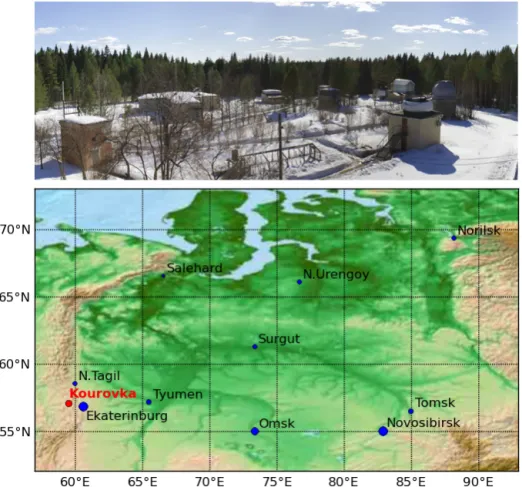
The atmospheric monitoring station of Kourovka was es-tablished in 2009 at the Kourovka astronomical observatory (Fig. 1), which was founded in 1965 as part of the Ural Federal University (the former Ural State University). It is located close to the western boundary of western Siberia (57.037◦N, 59.547◦E; 300 m a.s.l.), it is surrounded by pris-tine peatland, and is far from any large city (∼ 70 km from Ekaterinburg). There is no industry or any industrial dis-charge nearby. The observatory is situated in a clearing 100 m×100 m, within dense pine forest with an approxi-mate height of 15 m. Local cliapproxi-mate is continental. Based on published data for the region, over the past half-century the monthly mean temperatures range from −16◦C (January) to
+17◦C (July) with ∼ 460 mm of annual precipitation, peak-ing in summer (Shalaumova et al., 2010). The site is located
∼500 km to the south of the permafrost zone. The observa-tory infrastructure provides all the means needed to keep a
V. Bastrikov et al.: Continuous measurements of atmospheric water vapour isotopes 1765Discussion P ap er | Discussion P ap er | Discussion P ap er | Di scuss ion P ap er |
Fig. 1. Top to bottom: view of Kourovka astronomical observatory, map of Western Siberia (from the Ural Mountains on the west to the river Yenisei on the east) showing the location of major cities (blue circles) and the observatory (red circle).
28
Figure 1. Top to bottom: view of Kourovka astronomical observatory, map of western Siberia (from the Ural Mountains on the west to the
river Yenisei on the east) showing the location of major cities (blue circles) and the observatory (red circle).
constant year round temperature regime at the device area, non-interruptive power supply and protection from vandal-ism.
2.2 Meteorological data
Since July 2012, a meteorological station MetPak-II (Gill Instruments Ltd., Lymington, UK) has provided high-frequency (1 Hz) continuous measurement of the following atmospheric variables: barometric pressure (±0.05 kPa), rel-ative humidity (±0.8 % at 23◦C), air temperature (±0.1◦C), wind speed (±2 % at 12 m s−1), wind direction (±3◦ at 12 m s−1) and dew point temperature (±0.15◦C). These data are used to compare the humidity measurements performed by the isotope analyzer with meteorological measurements and to investigate the relationships between water vapour isotopic composition at the surface and local meteorological data (see Sects. 4.2 and 4.3).
2.3 Isotopic measurement set-up
Water vapour isotopic composition is measured with the laser spectroscopy analyzer L2130-i (Picarro Inc., Sunnyvale, CA, USA) based on WS-CRDS (Brand et al., 2009; Crosson et al.,
2002). The instrument was installed in Kourovka in mid-March 2012 and has been providing high-frequency (∼ 1 Hz) continuous measurements of δD and δ18O since April 2012.
The analyzer is installed in an air conditioned room (tem-perature 18 ± 1◦C). A shielded air intake is installed on the roof of the building (8 m a.g.l.) and a heated 6 m in-let line (O’Brien optical quality stainless steel tube, 9.5 mm (3/8 inch) OD) is connected with the analyzer. A 5 L min−1 pump ensures quick transport of air through the inlet tube. Electric heat tracing (type HKSI, HORST GmbH, Lorsch, Germany) maintains the temperature of the tube at 55–60◦C over the entire tube length.
The analyzer is programmed to perform self-calibrations after every six hours of ambient air measurement using the automated Picarro standards delivery module (SDM). Each calibration is made with two reference water samples: DW (distilled water, δD = −96.4 ‰, δ18O = −12.76 ‰) and YEKA (Antarctic snow and distilled water mix, δD =
−289.0 ‰, δ18O = −36.71 ‰). Each reference sample is measured continuously for 30 min. A third depleted refer-ence sample DOMEC (water standard from Laboratoire des Sciences du Climat et de l’Environnement (LSCE), δD =
1766 V. Bastrikov et al.: Continuous measurements of atmospheric water vapour isotopes
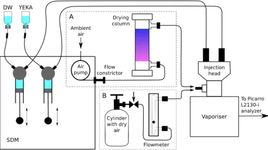
Figure 2. Illustration of the set-up used for (A) routine calibrations and (B) humidity–isotope response calibration.
assess the instrument linearity. The isotopic values of these reference waters in the VSMOW-SLAP scale were measured at LSCE by IRMS with accuracies of 0.5 ‰ for δD and 0.05 ‰ for δ18O.
An illustration of our calibration set-up is shown on Fig. 2. The liquid standard is drawn from container by syringe pump of the SDM and transferred via capillary line into the Picarro injection head (C0105) of the Picarro vaporisation module (A0211) which is set at 140◦C. Evaporated standard is then mixed with dried room air pumped at a rate of 12 L h−1 through a 450 cm3drying column filled with DRIERITE des-iccant (supplier no. 23001, W. A. Hammond Drierite Com-pany, Ltd., USA, www.drierite.com). The change of the des-iccant colour from blue to pink indicates when its activ-ity is depleted. Finally, the mixed standard water vapour is supplied into the Picarro analyzer. Adjustment of the reference water injection speed (between 0.002 µL s−1 and 0.08 µL s−1) allows water vapour concentration to be regu-lated within desired limits (in the range 800–30 000 ppmv). During calibration cycles, the humidity is usually set to 12 000 ppmv.
The following technical improvements of the standard Pi-carro configuration have been made:
– Substitution of the flexible metallised bags for reference
water standards with 15 mL glass bottles. This allows to visually control the absence of bubbles in the water, ab-sence of condensed water on the walls inside the bottle and remaining amount of the water standard. Condensed water could be easily removed from the walls by simple shaking, if needed. It is also easy to control the dryness of an empty bottle before filling it with the standard. The bottles are refilled to three-fourths of the volume once per week and installed in an upside down position. The water intake needle is introduced in the lower part of the bottle through the hole in the cap.
– Usage of disposable silicon septa inside the bottle
caps. This prevents bubble formation during insertion of a needle into the bottle.
– Replacement of ceramic syringe pumps with the newer
Picarro glass syringe pumps equipped with the soft plunger sealing (Tecan Systems, Inc., Ball-end 250 µL syringe, Ref. 19931 C X18A). This allows for the avoid-ance of air bubbling in the sealing between the plunger and syringe walls.
– At the humidity levels below 4000 ppmv, we observe
inconsistent calibration results (see Sect. 3.2) and thus substituted the air drying line (Fig. 2a) with the zero air gas supply from a 10 L tank cylinder (Fig. 2b). A cali-bration gas mixture of N2+O2(O2=20 % ±1 %) have been used (PGS-Service, Russia, www.pgs.ru) with the following content of impurities: H2≤0.0001 %, CO2≤0.0008 %, CO ≤ 0.0004 %, CH4 and other hy-drocarbons ≤ 0.0005 %, H2O at normal conditions
≤0.0002 %. The guaranteed dew point for the gas equals to −80◦C, which corresponds to approximately 0.5 ppmv of water vapour. For the flow rate control a purgemeter Sho-Rate 1350 with 3–65 Glass Tube (Serv’Instrumentation, France) have been used. The gas flow rate was kept within the range 10–35 L h−1.
3 Calibration protocol
In order to allow the water vapour measurements comparison with other data, it is important to perform a thorough char-acterisation of the individual instrumental system response. In this study we follow the calibration protocol described by Steen-Larsen et al. (2013). The major steps of the instrument calibration and data processing are discussed below. Prior to
V. Bastrikov et al.: Continuous measurements of atmospheric water vapour isotopes 1767 Discussion P ap er | Discussion P ap er | Discussion P ap er | Di scuss ion P ap er |
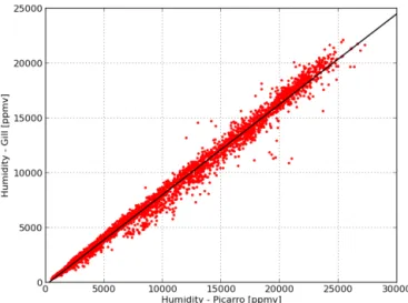
Fig. 3. Humidity measurements: Meteorological sensor (Gill Instruments) vs. Picarro. Black curve: linear fit (Eq. 3).
30
Figure 3. Humidity measurements: meteorological sensor (Gill
In-struments) vs. Picarro. Black curve: linear fit (Eq. 3).
these steps, we found it useful to perform a quality control of the raw data that includes the search and removal of random instrumental spikes in the data and artefacts due to power supply disturbances or other short-term technical problems.
3.1 Humidity correction
Picarro humidity measurements (absolute humidity mea-sured in ppmv) are compared to humidity values calculated from the Gill meteorological measurements (relative humid-ity and temperature) in Fig. 3. The best fit is given by a linear function (R2=0.992):
y = −231 + 0.825x, (3)
where x is the Picarro and y is the Gill humidity value (in ppmv), respectively. Equation (3) is hereafter used to trans-late all Picarro humidity data into the meteorological instru-ment scale.
In other studies, different results of comparing Picarro measurements with independent humidity observations have been reported. Aemisegger et al. (2012) also showed a lin-ear response of the analyzers when comparing to a dew point generator used to control humidity level in the range from 4000 to 31 000 ppmv. Tremoy et al. (2011) (in the range from 5000 to 36 000 ppmv) and Bonne et al. (2013) (in the range from 1000 to 18 000 ppmv) showed a non-linear response of the analysers compared to independent meteorological de-vice observations.
3.2 Humidity–isotope response calibration
The humidity–isotope response needs to be determined for each individual instrument, because isotopic measurements are sensitive to absolute water concentration (Steen-Larsen et al., 2013). The cause of this dependence is related to the spectral baseline being dependent on the height of the H216O
spectral peak. Non-perfect correction in the Picarro software for this influence means that a “manual” on-site characteri-sation is needed.
The instrument’s humidity–isotope response function was determined for the analyzer during its installation and is ver-ified several times a year. This calibration is established by introducing the two water standards (DW and YEKA) at dif-ferent humidity levels within the whole operational range. Resulting humidity–isotope response functions are shown in Fig. 4 (green – DW standard, blue – YEKA standard). The data are displayed for humidity levels below 5000 ppmv only, as the instrument response appears flat for higher levels. The
yaxis shows a bias with respect to the mean value measured at 12 000 ppmv. For the standard Picarro calibration set-up we obtained different humidity dependencies for δ18O mea-sured in different water standards and opposite dependencies for δD. The most plausible reason for this artefact is incom-plete air drying in the DRIERITE column. To confirm this hypothesis, a humidity calibration was performed with a sup-ply of dry gas from a tank cylinder rather than gas passed through the DRIERITE. The exact concentration of H2O in the filled container was measured as 0.5±0.1 ppmv. With this set-up, we obtained, within uncertainty, the same calibration curves for the two standards (red – DW standard, black – YEKA standard, with one conjoint fitting line shown in red). Moreover, the overall humidity dependency became signif-icantly less pronounced for the range 800–5000 ppmv. This indicates the importance of using “dry” air with very limited residual water vapour when performing calibrations at low humidity. Table 1 gives the analytical expressions used to ob-tain the best fit for the humidity–isotope response function in different cases and the associated coefficients.
Note that there are no data for the DRIERITE experiments below 800 ppmv due to the technical limitations of SDM. The behaviour of the humidity–isotope response functions for these conditions is therefore unknown.
Since all periodical self-calibrations were performed using dry air generated from DRIERITE, we used the humidity– isotope response functions from Eqs. (1)–(4) (Table 1) to correct the reference water sample measurements. To correct the ambient water vapour isotope measurements, we used the humidity–isotope response functions obtained using dry air (Table 1, Eqs. 5–6).
3.3 Known-standard calibration
For the period from June 2012 to September 2012, most of the instrument calibrations were invalidated due to a leakage in one of the standards delivery module syringes. The ce-ramic syringes of the SDM were replaced in September 2012 using a new type of glass syringe; this led to very stable and reproducible calibrations. The data discussed in this paper is therefore limited to the one-year period starting from 21 September 2012. The earlier data starting at the beginning of the instrument’s operation is limited to δD measurement.
1768 V. Bastrikov et al.: Continuous measurements of atmospheric water vapour isotopes Discussion P ap er | Discussion P ap er | Discussion P ap er | Di scuss ion P ap er |
Fig. 4. Picarro humidity–isotope response functions. Green error bars: calibration performed using DW standard and DRIERITE column, blue error bars: calibration performed using YEKA standard and DRIERITE column, red error bars: calibration performed using DW standard and dry gas, black er-ror bars: calibration performed using YEKA standard and dry gas. Solid lines represent linear fits to the data. For the measurements of DW and YEKA standards using dry air one conjoint fitting line is shown in red. The y-axis shows a bias with respect to the mean value measured at 12 000 ppmv.
31
Figure 4. Picarro humidity–isotope response functions. Green error bars: calibration performed using DW standard and DRIERITE column,
blue error bars: calibration performed using YEKA standard and DRIERITE column, red error bars: calibration performed using DW standard and dry gas, black error bars: calibration performed using YEKA standard and dry gas. Solid lines represent linear fits to the data. For the measurements of DW and YEKA standards using dry air one conjoint fitting line is shown in red. The y axis shows a bias with respect to the mean value measured at 12 000 ppmv.
Table 1. Humidity correction functions and coefficients for DW and YEKA standards.
N Standard Isotope Function a b
1 DW δ18O y = a ·exp(−x/b) 0.952 ± 0.153 1863 ± 344 2 (with DRIERITE) δD y = a + b/x 0.820 ± 0.107 −13 160 ± 315 3 YEKA δ18O y = a ·exp(−x/b) 3.770 ± 0.157 1653 ± 79 4 (with DRIERITE) δD y = a ·exp(−x/b) 6.224 ± 0.480 3270 ± 322 5 DW & YEKA δ18O y = a ·exp(−x/b) 8.394 ± 0.123 551.0 ± 11.3 6 (with dry gas) δD y = a ·exp(−x/b) −26.98 ± 3.80 140.4 ± 13.2
However, these limited results were compared well with model estimates and FTIR measurements (Gribanov et al., 2013).
During the first two winter months, the humidity level at which calibrations were performed was manually decreased to ∼ 4000 ppmv in order to reach a level close to the ambient air humidity. However, the instrumental noise induced a loss of accuracy in the calibrations (as reported in Sect. 3.2). We therefore set the humidity level back to ∼ 12 000 ppmv.
Figure 5 shows the complete set of calibrations con-ducted during the period from 21 September 2012 to 31 Au-gust 2013 with the VSMOW-SLAP slopes calculated from the measurements. Overall, 1672 calibrations have been made, among which 1552 (93 %) were successful (781 for DW standard and 771 for YEKA standard).
Two-standard calibrations were performed after every six hours of ambient air measurements. For each standard, the averaging window was selected within a steady plateau area,
usually during the last three minutes of the half-hour mea-surement. After each calibration, the first 13 min of ambient air measurements were discarded to ensure that any calibra-tion water vapour is purged out of the system. The length of these time periods was found to be reasonable for our par-ticular instrument on the basis of the measurement data. We refer the reader to the supplementary material for details.
Standard deviations calculated over the averaging win-dows range between: 0.4–2.5 ‰ for δD (with mean 0.9 ‰), 0.15–0.50 ‰ for δ18O (with mean 0.25 ‰) and 10–400 ppmv for humidity level (with mean 65 ppmv). Conversion of all humidity-corrected measurements to the VSMOW-SLAP scale upon known reference water samples have been per-formed at this step, assuming a linear instrumental drift be-tween calibrations and bracketing a given vapour measure-ment. Overall, the analyzer drift during the one-year pe-riod was < 2 ‰ for δD and < 0.5 ‰ for δ18O, resulting in
V. Bastrikov et al.: Continuous measurements of atmospheric water vapour isotopes 1769 Discussion P ap er | Discussion P ap er | Discussion P ap er | Di scuss ion P ap er |
Fig. 5. Picarro calibration data. Top to bottom: measured δ18O and δD values inh for DW standard (green dots) and YEKA standard (blue dots), calculated calibration slope for δ18O measurements (red dots) and δD measurements (purple dots), humidity concentration in ppmv (black dots).
32
Figure 5. Picarro calibration data. Top to bottom: measured δ18O and δD values in ‰ for DW standard (green dots) and YEKA standard (blue dots), calculated calibration slope for δ18O measurements (red dots) and δD measurements (purple dots), humidity concentration in ppmv (black dots).
VSMOW-SLAP slope change < 0.015 for δD and < 0.03 for
δ18O.
3.4 Total measurement uncertainty
Steen-Larsen et al. (2013) conservatively estimated the instrument precision and accuracy, when calibration was working properly, to be 1.4 ‰ for δD, 0.23 ‰ for
δ18O and 2.3 ‰ for d-excess at humidity levels between 1500 and 6000 ppmv, respectively. Following Steen-Larsen et al. (2013), we assume that we have similar precision and accuracy at these humidity levels and conservatively decide to use them for higher humidity levels.
At lower humidity levels, we observe an increase of the standard deviation of our measurements (see Fig. 4, red and black error bars) by a factor 4 at 1000 ppmv and a factor 8 at 500 ppmv. We therefore estimate the uncertainty between 1000 and 1500 ppmv to be 5.6 ‰ for δD, 0.92 ‰ for δ18O and 9.2 ‰ for d-excess, and between 500 and 1000 ppmv to be 11.2 ‰ for δD, 1.84 ‰ for δ18O and 18.5 ‰ for d-excess. Subsequently we decided not to report any measurements for values below 500 ppmv.
Such low humidity levels are encountered at Kourovka during winter. In total, 16 % of all hourly measurements have been made at humidity levels < 1500 ppmv (42 % of the win-ter measurements) and 2.5 % of the measurements have been made at humidity levels < 500 ppmv (6.4 % of the winter
measurements). In order to indicate the total uncertainty of the final calibrated data, a specific quality flag has been as-signed to each measurement depending on the relevant hu-midity level.
4 Results and discussions
Our Picarro isotopic analyzer has been operated continu-ously since April 2012 with only occasional short gaps due to electricity interruptions and minor breakdowns. Overall, for the reported period from 21 September 2012 to 31 Au-gust 2013, 6794 hourly Picarro measurements have been obtained, which corresponds to 82 % of the total duration (8280 h). The hourly averaged Picarro humidity and isotopic data and Gill meteorological data are presented in Fig. 6, af-ter applying all the corrections and calibrations discussed in the previous section.
Humidity concentration varies from ∼ 250 ppmv in win-ter up to ∼ 23 000 ppmv in summer, and co-varies with local surface air temperature. The seasonal cycle of δD and δ18O is parallel with the seasonal cycle of humidity and temper-ature, with the respective ranges of variation being −103 ‰ to −300 ‰ and −14 ‰ to −39 ‰. Maximum values are ob-served in summer (August), and minimum values in winter (January).
1770 V. Bastrikov et al.: Continuous measurements of atmospheric water vapour isotopes Discussion P ap er | Discussion P ap er | Discussion P ap er | Di scuss ion P ap er |
Fig. 6. Isotopic and meteorological measurements at Kourovka site. Top to bottom: d-excess, δ18O and δD inh, humidity concentration in ppmv, pressure in kPa, relative humidity in %, and temperature in ◦C. Deuterium excess values are not reported before September 2012, due to instabilities of calibrations during this period.
33
Figure 6. Isotopic and meteorological measurements at Kourovka site. Top to bottom: d-excess, δ18O and δD in ‰, humidity concentration in ppmv, pressure in kPa, relative humidity in %, and temperature in◦C. Deuterium excess values are not reported before September 2012, due to instabilities of calibrations during this period.
In addition to the seasonal pattern, significant variations are observed on a timescale of several days with respective magnitudes of 3000–8000 ppmv, 50–100 ‰, 10–15 ‰ and 2–8 ‰ in humidity, δD, δ18O and d-excess.
Deuterium excess values are only reported after Septem-ber 2012, due to the instabilities in the calibrations during the first months of measurement. They show a lagged seasonal cycle, with maximum values in winter (∼ 20 ‰) and mini-mum values in summer (∼ 5 ‰ during the day and ∼ −25 ‰ during the night). On a day-to-day basis, deuterium excess variations have a magnitude of less than 3 ‰. Opposite to this, the summer deuterium excess variability is much larger at the diurnal scale; this feature is further investigated in Sect. 4.3.
Our observed seasonal cycles in isotopes are consistent with earlier results obtained from northeast Siberia precipita-tion data by Kurita (2011). His record showed the peak δ18O occurring in late summer, and minimum in miwinter; his d-excess values decrease strongly during summer months, also reaching negative values. However, the maximum d-excess values were observed during mid-autumn and were attributed to increased kinetic effects due to the Artic-origin air mass contribution during this period. Yet this feature does not ap-pear in our 2012 record. Extending the Kourovka record over several years would allow the average seasonal cycle to be established and this contribution to be analysed.
Table 2. δD vs. δ18O (linear fit parameters for hourly averaged data).
Period N Slope Intercept R2 All data 6787 7.49 ± 0.01 −1.94 ± 0.27 0.99 All data (daytime) 2542 7.74 ± 0.01 6.75 ± 0.30 0.99 Autumn 1362 7.20 ± 0.03 −5.78 ± 0.65 0.98 Winter 2619 7.73 ± 0.02 4.40 ± 0.78 0.98 Spring 1101 6.85 ± 0.05 −14.3 ± 1.2 0.94 Spring (daytime) 408 7.24 ± 0.06 −3.55 ± 1.28 0.98 Summer 1705 5.57 ± 0.07 −39.6 ± 1.4 0.76 Summer (daytime) 634 7.02 ± 0.06 −7.74 ± 1.22 0.95 4.1 δD vs. δ18O
Figure 7 shows the relationship between surface vapour δD and δ18O through the complete campaign period (left panel) and for each season (right panels). Fitted parameters are presented in Table 2. Here and after, seasons are defined as follows (based on Kourovka climate): 21 September– 27 November (Autumn, N = 1362), 28 November–31 March (Winter, N = 2619), 1 April–31 May (Spring, N = 1101) and 1 June–31 August (Summer, N = 1705).
V. Bastrikov et al.: Continuous measurements of atmospheric water vapour isotopes 1771 Discussion P ap er | Discussion P ap er | Discussion P ap er | Di scuss ion P ap er |
Fig. 7. δD vs. δ18O. Left panel: all measurements, right panels: seasonal measurements, red dots: day-time measurements (from 12:00 to 21:00 LT), green dots: all other measurements, dashed line: linear fit through daytime measurements of the graph, solid line: linear fit through all measurements of the graph. See Table 2 for calculations of determination coefficients and slopes.
34
Figure 7. δD vs. δ18O. Left panel: all measurements, right panels: seasonal measurements, red dots: daytime measurements (from 12:00 to 21:00 LT), green dots: all other measurements, dashed line: linear fit through daytime measurements of the graph, solid line: linear fit through all measurements of the graph. See Table 2 for calculations of determination coefficients and slopes.
The linear slope fitted through all the measurements (red and green dots on Fig. 7) equals 7.5 for the whole data set and varies for different seasons from the maximum value (7.7) in winter to the minimum value (5.6) in summer (solid lines on Fig. 7). For all seasons, strong coefficients of de-termination are observed (R2>0.94), with the exception of summer where the coefficient of determination is smaller (R2=0.76).
As we observe strong diurnal cycles in the measurements time series, the relationship between δD and δ18O have been analyzed separately for the daytime measurements. For this we take the measurements performed during the daytime pe-riod from 12:00 to 21:00 local time (hereafter LT), which is free from strong variability (red dots on Fig. 7). In this case, we observe significant change of the slopes for spring (from 6.9 to 7.2) and summer (from 5.6 to 7.0) (dashed lines on Fig. 7) with higher coefficients of determination (R2>0.95). The overall value of the slope for the daytime measurements equals 7.7.
These results point out the significant role of local pro-cesses during the warm seasons in this region indicating a possible influence of continental recycling. During spring and summer, we observe both a loss of correlation and a change in slope, which are caused by the night measure-ments detachment from the overall strong correlation be-tween δD and δ18O. The reasons for this effect are discussed in Sect. 4.3.
Our slope values are comparable to the 6.8 value reported by Bonne et al. (2013) for the 1.5 year monitoring data in southern Greenland and the 6.5 value reported by Steen-Larsen et al. (2013) for NW Greenland in summer. In the latter work, separation of high d-excess measurements from the full data set also led to the higher slope values (7.4 for high d-excess measurements and 7.2 for non-high d-excess measurements).
4.2 δD vs. local meteorological data (humidity and temperature)
Figure 8 shows interdependencies of isotopic composition (δD) and meteorological data (temperature and humidity) for the full data set (left panels) and for each season (right pan-els) with fitted parameters presented in Table 3.
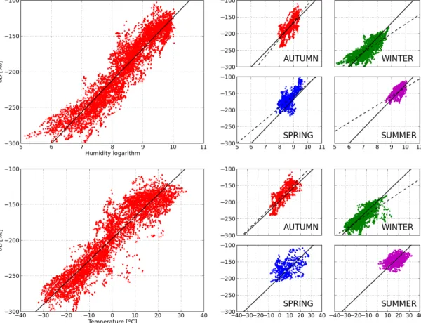
For δD, the strongest correlations are observed with the logarithm of humidity, which is consistent with what is ex-pected from Rayleigh distillation. We report R2=0.88 for all data, about 0.6 for autumn and winter, and 0.3–0.4 in spring and summer. The slopes are changing from 52 to 26 ‰ per log(humidity [ppmv]); the weakest ones can also be seen to occur in spring and summer.
A strong relationship is also observed between δD and temperature, as expected from the close relationship between temperature and logarithm of humidity, albeit less strong than the correlation with logarithm of humidity. We report
R2=0.84 for all data, about 0.6 for autumn and winter and much lower for spring and summer (0.15). The over-all relationship has a slope of 3.1 ‰◦C−1, with even lower isotope-temperature slopes in spring (1.0 ‰◦C−1) and sum-mer (0.9 ‰◦C−1).
For Rayleigh distillation, the slope between water vapour and temperature is very close to the slope between pre-cipitation isotopic composition and temperature and equals 0.8 ‰◦C−1for δ18O and 6 ‰◦C−1for δD. The overall slope value for our observations is about half the relationship ex-pected from Rayleigh distillation. Bonne et al. (2013) have analyzed the relationship between δ18O in vapour and local temperature for southern Greenland and obtained a slope of 0.37 ‰◦C−1, which is about half of the value expected from Rayleigh distillation. However, Steen-Larsen et al. (2014) observed the 0.81 ‰◦C−1value for the slope in NW Green-land during summer.
1772 V. Bastrikov et al.: Continuous measurements of atmospheric water vapour isotopesDiscussion P ap er | Discussion P ap er | Discussion P ap er | Di scuss ion P ap er |
Fig. 8. δD vs. logarithm-of-humidity (top) and δD vs. temperature (bottom). Left panels: all measure-ments, right panels: seasonal measuremeasure-ments, solid line: linear fit through all measuremeasure-ments, dashed line: linear fit through seasonal measurements. See Table 3 for calculations of determination coefficients and slopes.
35
Figure 8. δD vs. logarithm of humidity (top) and δD vs. temperature (bottom). Left panels: all measurements, right panels: seasonal
mea-surements, solid line: linear fit through all meamea-surements, dashed line: linear fit through seasonal measurements. See Table 3 for calculations of determination coefficients and slopes.
Table 3. δD vs. meteorological data (logarithm of humidity and temperature) (linear fit parameters for hourly averaged data).
Period N δD vs. logarithm of humidity δD vs. temperature
Slope Intercept R2 Slope Intercept R2
All data 6787 44.3 ± 0.2 −566 ± 2 0.88 3.06 ± 0.02 −197 ± 0.3 0.84 Autumn 1362 52.2 ± 1.2 −634 ± 10 0.59 3.19 ± 0.08 −189 ± 0.6 0.60 Winter 2619 29.7 ± 0.4 −464 ± 3 0.65 2.23 ± 0.04 −215 ± 0.6 0.56 Spring 1101 35.9 ± 1.3 −480 ± 11 0.42 – – 0.16 Summer 1705 26.5 ± 0.9 −397 ± 8 0.35 – – 0.15
Our data indicate that while local temperature is a key driver of autumn–winter seasonal variations of δD, which is consistent with temperature-driven distillation effects, this is not the case for spring–summer. During these seasons, the data depict a persistent but weaker relationship with loga-rithm of humidity (accounting for about 30 % of the vari-ance), and a minor impact of temperature. We conclude that in spring–summer local processes controlling local humidity variations are independent of surface temperature and may be related to continental recycling and local evapotranspiration (Welp et al., 2012; Berkelhammer et al., 2013), or convective activity.
4.3 Diurnal variations
The period from May to September is characterised by the frequent occurrence of days with a strong diurnal d-excess cycle, which is not seen during other seasons (Fig. 6). This diurnal variability arises from small variations in humidity (1000–3000 ppmv) and δ18O (1–5 ‰), but with no counter-part in δD. This diurnal decoupling between δD and δ18O contrasts with the overall strong correlation depicted at the daily to seasonal scale (Fig. 7).
Following the analysis of Berkelhammer et al. (2013), we have performed an objective cluster analysis to characterise dominant diurnal cycle patterns. SciPy k-means clustering
V. Bastrikov et al.: Continuous measurements of atmospheric water vapour isotopes 1773
routines have been used (Jones et al., 2001). The k-means clustering algorithm is one of the most used methods for vector quantisation. It is an iterative procedure, which par-titions n observations into k clusters trying to minimise the sum of the squared distances between each observation and corresponding cluster. The starting centroids for each of the clusters are randomly chosen. At each iteration the centre of mass is recomputed for each cluster obtained in the previous step and observations are redistributed between the clusters in accordance with which of the new centre is nearer.
For the clustering analysis we have used only diurnal cy-cles, which are more than two-thirds complete. We focus on the period 8 May 2013 to 31 August 2013 giving us 104 nearby complete diurnal cycles. The data have been averaged on the 15 min basis. We chose not to normalise or detrend the data and varied the number of clusters. However, we did not obtained significant difference between the clusters when we tried to partition the cycles into more than two clusters. Whereas for the two-clusters calculation, the difference be-tween the minimum d-excess values of the clusters (15 ‰) was 2.9 times larger than the standard deviation of the clus-ters. We have also performed an analysis of the meteorologi-cal conditions associated with each cluster. Here, we present the dominant patterns for d-excess, humidity and wind speed only and refer the reader to the Supplement for temperature, relative humidity, pressure and wind direction.
Figure 9 shows the dominant clusters for d-excess, humid-ity and wind speed. The red line (Cluster 1, 47 cycles) and the blue line (Cluster 2, 57 cycles) indicate the mean val-ues of each cluster, with corresponding standard deviations shown by shading. The yellow bars show the time of sun-rise (changing between 05:12 LT, on 8 May and 07:05 LT on 31 August) and similarly the dark red bars show sun-set (changing between 21:07 LT on 8 May and 23:03 LT on 31 August). These two clusters show similar variability dur-ing the day, but differ by the magnitude of the d-excess night depletion (decrease of 21 ‰ and 7 ‰, respectively), related to the magnitude of the daily humidity peak level (increase of 2400 ppmv and 1000 ppmv, respectively) and the night mean wind speed (0.27 m s−1and 0.78 m s−1, respectively).
The observed diurnal d-excess variability is similar to that reported by Berkelhammer et al. (2013), albeit they seem to only observe clusters similar to Cluster 1 (red line) and not Cluster 2 (blue line). This difference can be explained by the fact that the measurements of Berkelhammer et al. were carried out inside a mature open canopy (LAI = 1.9) pon-derosa pine forest, while our measurements are carried out in a clearing of size 100 × 100 metres within the dense forest. We suggest that this allows turbulent night mixing to strongly reduce or even mask the diurnal cycle of d-excess caused by transpiration and dew formation. Within all the diurnal cy-cles, we observe an inverse correlation (R = −0.74, Fig. 10a) between the night mean wind speed (between 23:00 LT and 07:00 LT) and the magnitude of d-excess drop (difference be-tween d-excess mean value for the interval from 15:00 LT to
Discussion
P
ap
er
|
Discussion
P
ap
er
|
Discussion
P
ap
er
|
Di
scuss
ion
P
ap
er
|
Fig. 9. Dominant clusters for (a) d-excess, (b) humidity and (c) wind speed. Yellow bars: sunrise time,
dark red bars: sunset time. The shading shows the standard deviation for each cluster.
36
Figure 9. Dominant clusters for (a) d-excess, (b) humidity and (c)
wind speed. Red line: Cluster 1, blue line: Cluster 2, yellow bars: sunrise time, dark red bars: sunset time. The shading shows the stan-dard deviation for each cluster.
18:00 LT and mean value for the interval from 07:00 LT to 08:00 LT).
Similar d-excess diurnal cycles had also been reported by Welp et al. (2012) in the meta-analysis of water vapour mea-surements from six different sites located in various ecosys-tems (forest, grassland, agricultural and urban settings), all of which showed the general feature of d-excess midday in-crease with remarkably similar phases in the time progres-sion. Throughout all the studies mentioned, the magnitude of d-excess daily variations ranges from ∼ 5 ‰ to ∼ 20 ‰ from site to site, but all share the same timing (decrease during the evening and the night with more rapid recovery in the morn-ing).
1774 V. Bastrikov et al.: Continuous measurements of atmospheric water vapour isotopes
Figure 10. Deuterium excess drop vs. (a) night mean wind speed and (b) morning humidity burst.
Within all the diurnal cycles, we observe a positive cor-relation (R = 0.49, Fig. 10b) between the magnitude of d-excess drop and the humidity value increase during the morn-ing burst (difference between humidity mean value for the interval from 09:30 LT to 10:30 LT and mean value for the in-terval from 05:00 LT to 06:00 LT). This finding is consistent with the mechanism proposed by Berkelhammer et al. (2013) whereby the diurnal d-excess cycle is a result of dew-fall and vapour-liquid interaction within the canopy. The morning burst is caused by initiation of transpiration and one would therefore expect (as our data also show) a positive correla-tion between the magnitude of d-excess drop and release of humidity in the morning.
5 Conclusions and perspectives
This study reports the successful use of a Picarro Inc. wa-ter vapour WS-CRDS analyzer for atmospheric wawa-ter vapour isotope measurements at the surface in western Siberia (Kourovka, Russia). The measurement system and calibra-tion protocol had been specifically adapted for the reliable performance at low humidity levels. Overall, the instrument demonstrated its ability to produce reliable measurements with an overall drift of less than 2 ‰ and 0.5 ‰ for δD and
δ18O, respectively. Frequent calibrations reveal a good repro-ducibility with standard deviations of 0.9 ‰ and 0.25 ‰ for
δD and δ18O, respectively.
At low humidity concentrations the measurements are subject to large errors. In particular, the Picarro standards delivery module requires further optimisation if it is to give reasonable calibration results for humidity levels be-low 4000 ppmv. We demonstrate that using dry air instead of DRIERITE produces excellent reproducibility for the isotope–humidity calibration curve established when using different standards.
During the monitoring campaign the isotopic composition varies in the range from −100 ‰ to −300 ‰ for δD, from
−15 ‰ to −40 ‰ for δ18O and from +25 ‰ to −25 ‰ for d-excess with the humidity concentration being in the range
250–23 000 ppmv. The data set reveals considerable seasonal variations of isotopic composition and humidity concentra-tion with a strong dependency on weather condiconcentra-tions. The strongest links are observed between δD and logarithm of humidity, and with temperature. However, these relationships are much weaker in spring–summer, especially for tempera-ture.
The summer period shows a strong diurnal variability of d-excess, which was not seen during other seasons. This vari-ability has a distinct relationship with sunset and sunrise and is consistent with interactions of dew-fall and canopy liq-uids with the atmospheric water vapour isotopes. During the night-time, d-excess experiences a strong decrease to nega-tive values with the minimum occurring close to sunrise, after which it returns to the value affected by synoptic variability. By means of objective cluster analysis, two dominant pat-terns for d-excess are distinguished and associated patpat-terns for meteorological parameters are determined. An inverse correlation is observed between the magnitude of d-excess diurnal decrease and the night wind speed and a positive cor-relation with the morning release of humidity.
The data obtained in this study provide a firm basis for further research of the atmospheric hydrological cycle of western Siberia. They are now available for comparison with remote-sensing measurements, outputs from moisture trajec-tory calculations, simulations of water vapour isotopic com-position from land surface and boundary-layer models, or at-mospheric general circulation models.
The work is part of a project investigating the water and carbon cycles in the permafrost and pristine peatlands of western Siberia and their projected changes under global warming. The full data set of isotopic and meteorological measurements discussed in this paper is available on the of-ficial site of the project WSibIso (“Impact of climate change on water and carbon cycles of melting permafrost of western Siberia”): http://www.wsibiso.ru, and in the web database of water isotope monitoring data: http://waterisotopes.lsce.ipsl. fr.
V. Bastrikov et al.: Continuous measurements of atmospheric water vapour isotopes 1775 The Supplement related to this article is available online
at doi:10.5194/amt-7-1763-2014-supplement.
Acknowledgements. This research was supported by the grant of
the Russian government under the contract 11.G34.31.0064. The authors thank John Gash for valuable edits and the anonymous reviewers for valuable suggestions during the review process, which improved the final version of this manuscript.
Edited by: A. Zahn
The publication of this article is financed by CNRS-INSU.
References
Aemisegger, F., Sturm, P., Graf, P., Sodemann, H., Pfahl, S., Knohl, A., and Wernli, H.: Measuring variations of δ18O and δ2H in atmospheric water vapour using two commercial
laser-based spectrometers: an instrument characterisation study, At-mos. Meas. Tech., 5, 1491–1511, doi:10.5194/amt-5-1491-2012, 2012.
Aemisegger, F., Pfahl, S., Sodemann, H., Lehner, I., Seneviratne, S. I., and Wernli, H.: Deuterium excess as a proxy for continental moisture recycling and plant transpiration, Atmos. Chem. Phys., 14, 4029–4054, doi:10.5194/acp-14-4029-2014, 2014.
Baer, D. S., Paul, J. B., Gupta, M., and O’Keefe, A.: Sensitive ab-sorption measurements in the near-infrared region using off-axis integrated-cavity output spectroscopy, Appl. Phys. B-Lasers O., 75, 261–265, 2002.
Barkan, E. and Luz, B.: Diffusivity fractionations of H162 O/H172 O and H162 O/H182 O in air and their implications for iso-tope hydrology, Rapid Commun. Mass Sp., 21, 2999–3005, doi:10.1002/rcm.3180, 2007.
Berkelhammer, M., Hu, J., Bailey, A., Noone, D. C., Still, C. J., Barnard, H., Gochis, D., Hsiao, G. S., Rahn, T., and Turnipseed, A.: The nocturnal water cycle in an open-canopy forest, J. Geophys. Res.-Atmos., 118, 10225–10242, doi:10.1002/jgrd.50701, 2013.
Bonne, J.-L., Masson-Delmotte, V., Cattani, O., Delmotte, M., Risi, C., Sodemann, H., and Steen-Larsen, H. C.: The iso-topic composition of water vapour and precipitation in Ivit-tuut, southern Greenland, Atmos. Chem. Phys., 14, 4419–4439, doi:10.5194/acp-14-4419-2014, 2014.
Brand, W. A., Geilmann, H., Crosson, E. R., and Rella, C. W.: Cav-ity ring-down spectroscopy versus high-temperature conversion isotope ratio mass spectrometry; a case study on δ2H and δ18O of pure water samples and alcohol/water mixtures, Rapid Commun. Mass Sp., 23, 1879–1884, doi:10.1002/rcm.4083, 2009. Butzin, M., Werner, M., Masson-Delmotte, V., Risi, C.,
Franken-berg, C., Gribanov, K., Jouzel, J., and Zakharov, V. I.: Vari-ations of oxygen-18 in West Siberian precipitation during the
last 50 yr, Atmos. Chem. Phys. Discuss., 13, 29263–29301, doi:10.5194/acpd-13-29263-2013, 2013.
Ciais, P. and Jouzel, J.: Deuterium and oxygen 18 in precipitation: isotopic model, including mixed cloud processes, J. Geophys. Res.-Atmos., 99, 16793–16803, 1994.
Craig, H.: Standard for reporting concentrations of deuterium and oxygen-18 in natural waters, Science, 133, 1833–1834, 1961. Craig, H. and Gordon, L.: Deuterium and oxygen-18 variations
in the ocean and marine atmosphere, in: Stable Isotopes in Oceanography Studies and Paleotemperatures, 26–30 July 1965, Spoleto, Italy, 1965.
Crosson, E. R., Ricci, K. N., Richman, B. A., Chilese, F. C., Owano, T. G., Provencal, R. A., Todd, M. W., Glasser, J., Kachanov, A. A., Paldus, B. A., Spence, T. G., and Zare, R. N.: Stable isotope ratios using cavity ring-down spectroscopy: Deter-mination of13C/12C for carbon dioxide in human breath, Anal. Chem., 74, 2003–2007, doi:10.1021/ac025511d, 2002.
Dansgaard, W.: Stable isotopes in precipitation, Tellus, 16, 436– 468, doi:10.1111/j.2153-3490.1964.tb00181.x, 1964.
Ellehoj, M. D., Steen-Larsen, H. C., Johnsen, S. J., and Mad-sen, M. B.: Ice-vapor equilibrium fractionation factor of hydro-gen and oxyhydro-gen isotopes: experimental investigations and impli-cations for stable water isotope studies, Rapid Commun. Mass Sp., 27, 2149–2158, doi:10.1002/rcm.6668, 2013.
Farlin, J., Lai, C.-T., and Yoshimura, K.: Influence of synoptic weather events on the isotopic composition of atmospheric mois-ture in a coastal city of the western United States, Water Resour. Res., 49, 3685–3696, doi:10.1002/wrcr.20305, 2013.
Farquhar, G. D., Cernusak, L. A., and Barnes, B.: Heavy water frac-tionation during transpiration, Plant Physiol., 143, 11–18, 2007. Field, R. D., Jones, D. B. A., and Brown, D. P.: Effects of
postcondensation exchange on the isotopic composition of wa-ter in the atmosphere, J. Geophys. Res.-Atmos., 115, D24305, doi:10.1029/2010JD014334, 2010.
Galewsky, J., Rella, C., Sharp, Z., Samuels, K., and Ward, D.: Sur-face measurements of upper tropospheric water vapor isotopic composition on the Chajnantor Plateau, Chile, Geophys. Res. Lett., 38, L17803, doi:10.1029/2011GL048557, 2011.
Gat, J. R.: Oxygen and hydrogen isotopes in the hydrological cycle, Annu. Rev. Earth Pl. Sc., 24, 225–262, 1996.
Gonfiantini, R.: Standards for stable isotope measurements in natu-ral compounds, Nature, 271, 534–536, 1978.
Gribanov, K., Jouzel, J., Bastrikov, V., Bonne, J.-L., Breon, F.-M., Butzin, F.-M., Cattani, O., Masson-Delmotte, V., Rokotyan, N., Werner, M., and Zakharov, V.: ECHAM5-wiso water vapour isotopologues simulation and its comparison with WS-CRDS measurements and retrievals from GOSAT and ground-based FTIR spectra in the atmosphere of Western Siberia, Atmos. Chem. Phys. Discuss., 13, 2599–2640, doi:10.5194/acpd-13-2599-2013, 2013.
Gryazin, V., Risi, C., Jouzel, J., Kurita, N., Worden, J., Franken-berg, C., Bastrikov, V., Gribanov, K., and Stukova, O.: The added value of water isotopic measurements for understanding model biases in simulating the water cycle over Western Siberia, At-mos. Chem. Phys. Discuss., 14, 4457–4503, doi:10.5194/acpd-14-4457-2014, 2014.
Gupta, P., Noone, D., Galewsky, J., Sweeney, C., and Vaughn, B. H.: Demonstration of high-precision continuous measurements of water vapor isotopologues in laboratory and remote field
deploy-1776 V. Bastrikov et al.: Continuous measurements of atmospheric water vapour isotopes
ments using wavelength-scanned cavity ring-down spectroscopy (WS-CRDS) technology, Rapid. Commun. Mass. Sp., 23, 2534– 2542, 2009.
Han, L.-F., Groening, M., Aggarwal, P., and Helliker, B. R.: Reli-able determination of oxygen and hydrogen isotope ratios in at-mospheric water vapour adsorbed on 3A molecular sieve, Rapid. Commun. Mass. Sp., 20, 3612–3618, doi:10.1002/rcm.2772, 2006.
IAEA: Final Report on Fourth interlaboratory comparison exercise for δ2H and δ18O analysis of water samples (WICO2011), Inter-national Atomic Energy Agency (IAEA), 2012.
Jacob, H. and Sonntag, C.: An 8-year record of the seasonal varia-tion of2H and18O in atmospheric water vapour and precipitation at Heidelberg, Germany, Tellus B, 43, 291–300, 1991.
Jones, E., Oliphant, T., and Peterson, P. SciPy: Open source scien-tific tools for Python, available at: http://www.scipy.org/, 2001– 2014.
Jouzel, J.: Isotopes in cloud physics: Multistep and multistage pro-cesses, The Terrestrial Environment B, edited by: Fritz, P. and Fontes, J. C., Vol. 2, Handbook of Environmental Isotopes Geo-chemistry, Elsevier, 61–112, 1986.
Kerstel, E. R. T. and Gianfrani, L.: Advances in laser-based isotope ratio measurements: selected applications, Appl. Phys. B-Lasers O., 92, 439–449, 2008.
Kerstel, E. R. T., van Trigt, R., Dam, N., Reuss, J., and Mei-jer, H. A. J.: Simultaneous determination of the2H/1H,17O/16O, and18O/16O isotope abundance ratios in water by means of laser spectrometry, Anal. Chem., 71, 5297–5303, 1999.
Kurita, N.: Origin of Arctic water vapor during the ice-growth season, Geophys. Res. Lett., 38, L02709, doi:10.1029/2010GL046064, 2011.
Kurita, N., Newman, B. D., Araguas-Araguas, L. J., and Aggarwal, P.: Evaluation of continuous water vapor δD and δ18O measure-ments by off-axis integrated cavity output spectroscopy, Atmos. Meas. Tech., 5, 2069-2080, doi:10.5194/amt-5-2069-2012, 2012. Kurita, N., Fujiyoshi, Y., Wada, R., Nakayama, T., Matsumi, Y., Hiyama, T. and Muramoto, K.: Isotopic variations associated with North-South displacement of the Baiu front, SOLA, 9, 187– 190, 2013.
Kurita, N., Yoshida, N., Inoue, G., and Chayanova, E. A.: Modern isotope climatology of Russia: a first assessment, J. Geophys. Res.-Atmos., 109, D03102, doi:10.1029/2003JD003404, 2004. Majoube, M.: Fractionnement en oxygène 18 et en deutérium entre
l’eau et sa vapeur, J. Chim. Phys., 68, 1423–1436, 1971. Merlivat, L.: Molecular diffusivities of H162 O, HD16O and H182 O in
gases, J. Chem. Phys., 69, 2864–2871, 1978.
Merlivat, L. and Jouzel, J.: Global climatic interpretation of the deuterium-oxygen 18 relationship for precipitation, J. Geophys. Res.-Oceans, 84, 5029–5033, doi:10.1029/JC084iC08p05029, 1979.
Merlivat, L. and Nief, G.: Fractionnement isotopique lors des changements d’état solide-vapeur et liquide-vapeur de l’eau à des températures inférieures à 0◦C, Tellus, 19, 122–127, doi:10.1111/j.2153-3490.1967.tb01465.x, 1967.
Rozanski, K., Araguás-Araguás, L., and Gonfiantini, R.: Iso-topic patterns in modern global precipitation, in: Geophraphi-cal Monograph Series, edited by: Swart, P. K., Lohmann, K. C., McKenzie, J., and Savin, S., Vol. 78, American Geophysical Union, Washington DC, 1–36, 1993.
Shalaumova, Y. V., Fomin, V. V., and Kapralov, D. S.: Spatiotempo-ral dynamics of the USpatiotempo-rals climate in the second half of the 20th century, Russ. Meteorol. Hydrol., 35, 107–114, 2010.
Steen-Larsen, H. C., Johnsen, S. J., Masson-Delmotte, V., Stenni, B., Risi, C., Sodemann, H., Balslev-Clausen, D., Blu-nier, T., Dahl-Jensen, D., Ellehøj, M. D., Falourd, S., Grind-sted, A., Gkinis, V., Jouzel, J., Popp, T., Sheldon, S., Simon-sen, S. B., Sjolte, J., SteffenSimon-sen, J. P., Sperlich, P., Sveinbjörns-dóttir, A. E., Vinther, B. M., and White, J. W. C.: Continuous monitoring of summer surface water vapor isotopic composition above the Greenland Ice Sheet, Atmos. Chem. Phys., 13, 4815– 4828, doi:10.5194/acp-13-4815-2013, 2013.
Steen-Larsen, H. C., Masson-Delmotte, V., Hirabayashi, M., Win-kler, R., Satow, K., Prié, F., Bayou, N., Brun, E., Cuffey, K. M., Dahl-Jensen, D., Dumont, M., Guillevic, M., Kipfstuhl, S., Landais, A., Popp, T., Risi, C., Steffen, K., Stenni, B., and Sveinbjörnsdottír, A. E.: What controls the isotopic compo-sition of Greenland surface snow?, Clim. Past, 10, 377–392, doi:10.5194/cp-10-377-2014, 2014.
Stewart, M. K.: Stable isotope fractionation due to evaporation and isotopic exchanges of falling water drops: applications to atmo-spheric processes and evaporation of lakes, J. Geophys. Res., 80, 1133–1146, 1975.
Strong, M. Z. D., Sharp, D., and Gutzler, D. S.: Diagnosing moisture transport using D/H ratios of water vapor, Geophys. Res. Lett., 34, L03404, doi:10.1029/2006GL028307, 2007.
Sturm, P. and Knohl, A.: Water vapor δ2H and δ18O
measure-ments using off-axis integrated cavity output spectroscopy, At-mos. Meas. Tech., 3, 67–77, doi:10.5194/amt-3-67-2010, 2010. Tremoy, G., Vimeux, F., Cattani, O., Mayaki, S., Souley, I., and
Favreau, G.: Measurements of water vapor isotope ratios with wavelength-scanned cavity ring-down spectroscopy technology: new insights and important caveats for deuterium excess mea-surements in tropical areas in comparison with isotope-ratio mass spectrometry, Rapid Commun. Mass Sp., 25, 3469–3480, doi:10.1002/rcm.5252, 2011.
Tremoy, G., Vimeux, F., Mayaki, S., Souley, I., Cattani, O., Risi, C., Favreau, G., and Oi, M.: A 1-year long 18O record of wa-ter vapor in Niamey (Niger) reveals insightful atmospheric pro-cesses at different timescales, Geophys. Res. Lett., 39, L08805, doi:10.1029/2012GL051298, 2012.
Uemura, R., Matsui, Y., Yoshimura, K., Motoyama, H., and Yoshida, N.: Evidence of deuterium excess in water vapor as an indicator of ocean surface conditions, J. Geophys. Res.-Atmos., 113, D19114, doi:10.1029/2008JD010209, 2008.
Welp, L. R., Lee, X., Griffis, T. J., Wen, X.-F., Xiao, W., Li, S., Sun, X., Hu, Z., Martin, M. V., and Huang, J.: A meta-analysis of water vapor deuterium-excess in the midlatitude at-mospheric surface layer, Global Biogeochem. Cy., 26, GB3021, doi:10.1029/2011GB004246, 2012.
Wen, X.-F., Zhang, S.-C., Sun, X.-M., Yu, G.-R., and Lee, X.: Water vapor and precipitation isotope ratios in Beijing, China, J. Geo-phys. Res., 115, doi:10.1029/2009JD012408, 2011.