HAL Id: halshs-00575003
https://halshs.archives-ouvertes.fr/halshs-00575003
Preprint submitted on 9 Mar 2011
HAL is a multi-disciplinary open access
archive for the deposit and dissemination of
sci-entific research documents, whether they are
pub-lished or not. The documents may come from
teaching and research institutions in France or
L’archive ouverte pluridisciplinaire HAL, est
destinée au dépôt et à la diffusion de documents
scientifiques de niveau recherche, publiés ou non,
émanant des établissements d’enseignement et de
recherche français ou étrangers, des laboratoires
Asymptotic age structures and intergenerational trade
Grégory Ponthière
To cite this version:
WORKING PAPER N° 2009 - 34
Asymptotic age structures and
intergenerational trade
Grégory Ponthière
JEL Codes: J11, J13, J14
Keywords: Age structure, OLG model, fertility, mortality,
demographic transition, intergenerational trade
P
ARIS
-
JOURDAN
S
CIENCES
E
CONOMIQUES
L
ABORATOIRE D
’E
CONOMIE
A
PPLIQUÉE
-
INRA
48,BD JOURDAN –E.N.S.–75014PARIS TÉL. :33(0)143136300 – FAX :33(0)143136310
www.pse.ens.fr
CENTRE NATIONAL DE LA RECHERCHE SCIENTIFIQUE – ÉCOLE DES HAUTES ÉTUDES EN SCIENCES SOCIALES ÉCOLE NATIONALE DES PONTS ET CHAUSSÉES – ÉCOLE NORMALE SUPÉRIEURE
Asymptotic Age Structures and
Intergenerational Trade
Gregory Ponthiere
September 11, 2009
Abstract
While demographers Lotka (1939) and Lopez (1961) proposed condi-tions on (exogenous) fertility and mortality laws under which populacondi-tions with distinct initial age structures exhibit the same asymptotic age struc-ture, this paper re-examines the issues of age structure stabilization and convergence, by considering a population whose fertility and mortality are endogenously determined in the economy. For that purpose, we develop a three-period OLG model where human capital accumulation and inter-generational trade a¤ect fertility and longevity. It is shown that the age structure must converge asymptotically towards a stable structure, whose form depends on the structural parameters of the economy. Moreover, populations with distinct initial age structures will end up with the same long-run age structure when fertility and mortality laws are converging, which requires converging terms of trade between coexisting generations in the di¤erent populations under study.
Keywords: Age structure, OLG model, fertility, mortality, demographic transition, intergenerational trade.
JEL codes: J11, J13, J14
1
Introduction
The history of mankind is, among other things, a history of cooperations - and sometimes con‡icts - between coexisting generations. At any epoch, the coexis-tence of individuals of di¤erent ages generated its own set of intergenerational arrangements, duties and trades, whose goal was, quite often, to take advantage of the age heterogeneity.1 But the age heterogeneity is also an output of intergenerational relations, as fertility and longevity and thus the age structure -depend on the precise form of intergenerational settlements. Hence, the study of the long-run dynamics of economies and populations requires to consider the joint dynamics of age structures and intergenerational relations.
This paper aims precisely at developing a model of coexisting generations, whose relative sizes are both an output and an input of intergenerational re-lations. Our focus on the interplay between age heterogeneity and intergener-ational relations will allow us, in particular, to study major mechanisms lying behind the observed long-run dynamics of age structures.
Ecole Normale Supérieure, Paris and PSE. E-mail: [email protected]
1Such intergenerational settlements include, for instance, child care, education activities,
As this was stressed by demographers (see Lee, 2003), the age structure of populations has been evolving signi…cantly across epochs. While human societies were, at the middle of the 18th century, mainly composed of what can be roughly called ‘young’ persons, the share of the ‘young’ started falling during the second part of the 19th century in industrialized economies, whereas the shares of middle-aged and elderly people started growing, and kept growing even more during the 20th century. That evolution is illustrated on Figure 1 by the case of Sweden.2 The share of people younger than 35 years, which consisted of about 68 % of the population around 1850, started falling after 1850, and amounts today to only 42 % of the Swedish population.
0% 10% 20% 30% 40% 50% 60% 70% 80% 90% 100% 1751 1801 1851 1901 1951 2001
share of 0-34 year-old share of 35-69 year-old share of 70-104 year-old
Figure 1: Age structure in Sweden, 1751-2008
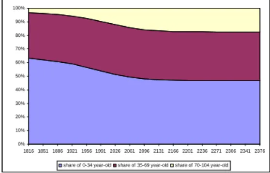
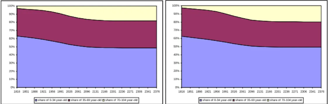
This non-constancy of the age structure is mainly due to large changes in fertility and mortality over time. Demographers regard the evolution of age structures as an outcome of the demographic transition process: human societies have, during the last two centuries, switched from a regime with a high fertility and a high mortality to a regime with a low fertility and a low mortality.3 The observed ageing of societies during the second part of the 19th century and the 20th century constitutes thus only a subproduct of those evolutions of births and deaths. Hence, all economies having experienced the demographic transition are also characterized by the evolution of age structure just described (see Figures 2 and 3 for England and Wales and France).4
In front of such sizeable evolutions of age structures over time, a natural question to raise is the one of the likelihood of a stabilization of age structures: can we expect that age structures will stabilize at some point in the future, and, if yes, what will the stable age structure look like? Another natural question is the one of the convergence of age structures across populations: will the long-run age structure be the same in all populations?
In what is still regarded today as a major result of theoretical demography, Alfred Lotka (1939) identi…ed conditions that are su¢ cient for the asymptotic stabilization of an age structure.5 The so-called Lotka Theorem states that,
2Sources: The Human Mortality DataBase (2008). See de la Croix, Lindh and Malmberg
(2009) for a study of long run demographic and economic changes in Sweden.
3See Lee (2003).
4Sources: The Human Mortality Database (2008).
0% 10% 20% 30% 40% 50% 60% 70% 80% 90% 100% 1841 1891 1941 1991
share of 0-34 year-old share of 35-69 year-old share of 70-104 year-old
Figure 2: Age structure in England and Wales, 1841-2006
0% 10% 20% 30% 40% 50% 60% 70% 80% 90% 100% 1816 1866 1916 1966
share of 0-34 year-old share of 35-69 year-old share of 70-104 year-old
Figure 3: Age structure in France, 1816-2008
provided (i) age-speci…c fertility rates are constant, (ii) age-speci…c death rates are constant, (iii) age-speci…c migration rates are zero, a population must nec-essarily end up, as time goes to in…nity, with a constant age structure, which is independent from the initial age structure and size of the population. Lotka Theorem states actually a result of strong convergence: populations tend, if sub-ject to the same, constant fertility and mortality laws, to "forget their past", which is a property known as strong ergodicity.6 That result, which concerns stable populations (i.e. subject to constant fertility and mortality laws), was generalized by Alvaro Lopez (1961) in the context of unstable populations (i.e. subject to varying fertility and mortality laws), in what is known as a weak convergence theorem. According to Lopez, if populations are subject to the same time-varying fertility and mortality laws, populations with distinct initial age structures must exhibit, in the long-run, the same age structure.
The importance of Lotka and Lopez’s results for the economic study of hu-a sthu-able populhu-ation structure, hu-as whether the populhu-ation size grows or fhu-alls depends ultimhu-ately on the relative strengths of mortality and fertility.
6Note that, as stressed by Preston et al (2001, p. 146), Lotka’s result can be extended to
the case of populations with the same age-speci…c migration rates, so that condition (iii) is not crucial for Lotka’s result.
man societies could hardly be overemphasized.7 On the descriptive side, the evolution of economic aggregates over time (production, consumption, savings, employment, etc.) is dependent on how the population is structured in terms of age.8 On the normative side, it is also clear that the age heterogeneity of populations is a major source of concern for policy making. Thus, there is a strong need to know under which conditions the age heterogeneity can stabilize. However, those two contributions, made at the highest level of generality, do not inform us about the precise form of the asymptotic age structure. To answer that question, one must add assumptions on how fertility and mortality are determined, and make explicit how these are in‡uenced by, among other things, the form of intergenerational relations. But, as we shall see, endogenizing fertility and mortality is not only relevant for characterizing asymptotic age structures, but, also, for the restatement of the conditions guaranteeing the convergence of age structure across populations.
For those purposes, we develop here a three-period overlapping genera-tions model (OLG) with human capital accumulation, where both fertility and longevity are endogenous, and analyze the dynamics of age structures under that theoretical framework.9 In that economy, the di¤erent generations that co-exist at each period of time are characterized by trade relations, in the spirit of the seminal model by Ehrlich and Lui (1991). Young adults, as parents, transfer resources to their children, in order to raise them and educate them, but they transfer also resources to their own parents, so that intergenerational trade is here oriented both downwards and upwards. But an important di¤erence with respect to the model of Ehrlich and Lui, in addition to the endogeneity of mor-tality, is that contribution rates to the children and the elderly are here not constants, but variables depending on the level of human capital.
While the literature includes several OLG models with both endogenous fertility and longevity (Blackburn and Cipriani, 2002; Gallor and Moav, 2005; de la Croix and Licandro, 2007; Strulik and Weisdorf, 2008), the speci…city of this paper is that it pays a particular attention to the dynamics of the age structure, and to its relationships with intergenerational trade. The present model shares with Blackburn and Cipriani (2002) the three-period OLG structure with human capital accumulation, but introduces intergenerational trade as a motive for fertility decision, and considers the interplay between intergenerational trade and age structure dynamics. The present paper shares also with Galor and Moav (2005) the presence of a pure taste for children in the fertility decision, but concentrates on age heterogeneity within the population rather than on heterogeneity within each cohort. Finally, endogenous fertility and mortality are also treated in a model of human capital accumulation by de la Croix and Licandro (2007) and Strulik and Weisdorf (2008), but they concentrate on a society without intergenerational trade, unlike the present framework.
Thus the particularity of this study is to concentrate on the interplay between age heterogeneity, intergenerational trade and human capital accumulation, in order to examine whether Lotka and Lopez’s stabilization and convergence re-sults remain true under endogenous fertility and mortality. It is shown that,
7On the relations between Lotka and Lopez’ results, see Challier and Michel (1996). 8For a recent empirical study of the impact of age-structure on GDP growth, see Lindh
and Malmberg (2009).
9As such, this paper complements other theoretical pieces of work concerned with the
if children are treated both as consumption goods and as investment goods by their parents, the age structure must asymptotically converge towards a stable structure, whose form depends on the structural economic and demographic pa-rameters characterizing the population. Moreover, it is shown that populations with distinct initial age structures exhibit the same asymptotic age structure, provided fertility and mortality laws are converging, which requires converging terms of trade between coexisting generations in the populations under study.
This paper is organized as follows. Section 2 presents the model. Section 3 examines the long-run production dynamics. The dynamics of age structures is studied in Section 4. Section 5 provides a numerical illustration on the basis of France (1816-2008), and extrapolates the long-run age structure under several postulates for the survival process. Section 6 concludes.
2
The model
2.1
Environment
Let us consider a three-period OLG model. Each period of life has a length normalized to 1.
All agents live the …rst period of life for sure. This consists of a period of childhood, during which the child does not produce anything, and bene…ts from the resources of his parent.
A proportion 1t+1of the cohort born at time t will enjoy the second period of life. That period is a period of young adulthood, during which agents work, help their parents and educate their children. Reproduction is monosexual.
Finally, only a proportion 2t+2of the part of the cohort that survived to the second period will reach the third period of life. That period is a period during which agents are retired, and live thanks to the generosity of their children.
In this model, life expectancy at birth is: (1 1
t+1)1 + 1t+1(1 2t+2)2 + 1
t+1 2t+2(3) = 1 + 1t+1+ 1t+1 2t+2.
Children born at time t inherit, during their …rst period of life, ht units of human capital from their parents.
2.2
Survival conditions
Survival conditions at all ages are assumed to be shaped by the current stock of human capital, i.e. the stock of knowledge prevailing at the time of existence of the agents.10 Formally, the probability of survival to the second period of life of a person born at t 1, denoted by 1
t, depends positively on the stock of human capital htby means of the survival function:
1
t 1(ht) (1)
where 1(h
t) exhibits the following properties: 1(:) 0, 10(:) > 0 and 100(:) < 0. We assume also that 1(h
t) is bounded from below and from above: limht!0
1(h
t) = ~1> 0 and limht!1
1(h
t) = 1< 1.
1 0This assumption di¤ers from the postulate according to which individual longevity
de-pends on the human capital stock prevailing at the birth of the agent. In our setting, agents do, on the contrary, bene…t from the advances of knowledge during their whole life.
Similarly, the probability of survival from the second to the third period of life, 2
t, depends positively on the stock of human capital: 2 t 2(ht) (2) with 2(:) 0, 20(:) > 0, 200(:) < 0, lim ht!0 20(h t) < 1, and limht!1 20(h t) = 0. We assume also limht!0
2(h
t) = ~2> 0 and limht!1
2(h
t) = 2< 1.
2.3
Production
At the young adult age, (surviving) agents produce a good, according to a technology that is assumed, for simplicity, to be linear in human capital:
yt= wht (3)
where yt denotes the output per head, while w is the wage per unit of human capital. For the sake of the presentation, this wage will be normalized to unity in the rest of this paper (i.e. w = 1).
The stock of human capital ht+1 depends on the past human capital ht, and on the amount of education expenditures that each adult dedicates to the education of each child, as follows
ht+1= A etht
nt
h1t (4)
where et is the fraction of parental income ht dedicated to education, nt is the number of children, A is a productivity parameter (A > 0), while is the elasticity of ht+1to education spending per child (i.e. 0 < < 1).
2.4
Agents’decisions
Young adults work during the second period, and decide the number of children nt and the fraction of their income dedicated to education et.11 But before considering those decisions, let us …rst specify intergenerational transfers.
Intergenerational transfers Following Ehrlich and Lui (1991), it is as-sumed that young adult agents must take care of their family: children (con-sumption and education) and old parents (con(con-sumption only). Contributions to the consumption of other family members are compulsory, and each young adult takes the family contribution rates as given.12
Each young adult must give a proportion t of his resources to each of his ntchildren, to cover food and clothing costs, as well as other expenditures (e.g. toys, leisure activities, travel, etc.). That fraction is a function of the level of human capital prevailing at the time of the birth of the child:
t (ht) (5)
where 0 < t < 1 for any ht. We thus allow here for a non-constancy of the (relative) child cost, which may vary with the level of human capital. The
1 1That decision structure is close to the one developed by Erhlich and Lui (1991), where
mortality is exogenous.
1 2This approach di¤ers from the one of Ehrlich and Lui (1991) in the basic version of their
(relative) contribution to each child is assumed to be bounded from below and from above: limht!0 (ht) = ~ > 0 and limht!1 (ht) = < 1. As far as
the precise shape of the function (ht) is concerned, a recent study by Farrell and Shields (2007) on the behaviour of children as consumers suggests that the contribution rate tis likely to be non decreasing in the level of income: 0(ht) 0. Actually, as shown by Farrell and Shields, while some goods, which represent a small share of children’s spending, such as drinks, sweets, toys and books, are normal goods, the goods that represent a larger share of their spending, such as clothes, travel, and leisure, are luxury goods (i.e. with an income elasticity larger than 1). In the present one-good model, the elasticity of expenditures per child with respect to parental income ht, which is equal to 1 +
0(h t)
(ht)ht, is
larger than 1 if and only if 0(h
t) 0. Hence we shall assume, throughout this paper, that the contribution rate tis non decreasing in ht.13
Regarding the help to the elderly, it is assumed, for simplicity, that all young adults must dedicate some …xed proportion of their resources to the old, surviving, cohort, through a social insurance system that pools the risks of having surviving elderly parents on the whole young adults cohort. Thus, each young adult, whatever his parent survives or not to the old age, dedicates a proportion t 2t of his resources to the old, surviving, cohort.14 As for the help to the children, that fraction t is a function of the level of human capital prevailing at the time of the retirement of the old:
t (ht) (6)
where 0 < t< 1 for any ht. Here again, the contribution rate is assumed to be bounded from below and from above: limht!0 (ht) = ~ > 0 and limht!1 (ht) =
< 1. As far as the shape of (ht) is concerned, it is reasonable, in the light, for instance, of the large empirical evidence on the rise of the cost of long term care (per dependent person) as the economy develops, to assume that the ex-penditure dedicated to the old is, like the exex-penditure dedicated to the young, a non decreasing function of income ht: 0(ht) 0.15
Budget constraints Each young adult earns an income ht by his work, and uses that income to help his children and parents. Moreover, a young adult spends a fraction et of his resources for the higher education of his children (0 et 1). That fraction is, unlike t, chosen by the adult agent. One can interpret that asymmetry as re‡ecting the fact that, as far as basic consumption is concerned, social norms and customs are strongly at work: each society pro-duces its norms regarding how one has to treat one’s children and one’s elderly parents, and those norms are strictly respected. However, parents bene…t from a much larger degree of freedom regarding (high) education spending.
Second-period consumption ctis what remains of labour income once inter-generational transfers and education spending have been paid:
ct= (1 tnt t 2t et)ht (7)
1 3We shall also assume, in the rest of this paper, that lim
ht!0 0(ht) < 1 and
limht!1 0(ht) = 0.
1 4It is only in the special case where there is no elderly people alive (i.e. 2
t= 0) that young
adults neglect the previous generation.
1 5On the rise of the LTC costs per dependent person, see Cutler (1996) and Norton (2000).
Precise …gures on the rise of the share of LTC expenditures in GDP can be found in a recent report by the European Commission (2009).
This is decreasing in the number of children, and decreasing in the proportion of survivors among the elderly, 2
t. Note, however, that, while the number of children ntis chosen by agents, the proportion of surviving elderly 2t is not.
A young adult expects also to consume, if he is still alive at the retirement age, a consumption dt+1, which comes exclusively from the contributions of the young cohort (for simplicity, there is no savings in this economy):
dt+1= t+1 2t+1ht+1
nt 1t+1 2 t+1
= nt 1t+1 t+1ht+1 (8)
The factor in brackets corresponds to what is given by each young adult at period t+1, while the second factor consists of the ratio of young adults over old adults. The impact of the young cohort’s contribution on the old’s consumption depends thus on the sizes of those two demographic groups.
Optimal fertility and education Agents’ preferences are assumed to take a standard log-linear form in second-period and third-period consumptions, and in the number of children. Agents are also supposed to be expected utility maximizers, with a zero utility from being dead. Moreover, at the time of their decisions, agents form myopic anticipations regarding future survival conditions, and thus believe that the probabilities 1
t+1and 2t+1are equal to the currently prevailing probabilities, i.e. 1
t and 2t. Similarly, agents take contributory rates tand t as given constants, even though these may evolve over time.16
Hence, if one abstracts from childhood, the expected lifetime welfare is:17 Ut= log(ct) + log(nt) + 2tlog(dt+1) (9) where captures the relative strength of the taste for children (0 < < 1). Note that this expression treats children as consumption goods and investment goods (through dt+1), but abstracts from any altruistic concerns.18
Substituting for consumption and for the resources at the old age yields: Ut= log((1 tnt t 2t et)ht) + log(nt) + 2tlog 1tn1t tAetht (10)
The …rst-order condition for optimal fertility is: nt=
( + 2
t(1 )) 1 t 2t
t(1 + + 2t)
(11) Optimal fertility is, without surprise, increasing in the taste for children , and decreasing in the cost per child t.19 It is also decreasing in the contribution
1 6Thus, the young adult expects to bene…t, once old, from the same relative aid as the one
he o¤ered when being young.
1 7We abstract here from pure time preferences. Actually, there is not really a need for these
in the present context, where the survival probability 2
t acts as a ‘natural’ discount factor,
assigning lower weight to future consumption on the grounds of its risky nature.
1 8This model di¤ers thus from Barro and Becker (1989), where altruism towards children
makes parent care about the utility of the whole dynasty following them. In the literature on endogenous fertility and mortality, see de la Croix and Licandro (2007) on the quality versus quantity trade-o¤, in a context where parents care about the survival of their children, unlike the present, purely egoistic context.
1 9Fertility is here strictly positive, as we have + 2
t(1 ) > 0for any level of 2t under
< 1. This interior solution di¤ers from Ehrlich and Lui (1991), where = 0and = 1, so that a corner solution with the minimum number of surviving children prevails, as the marginal net return for investing in the quality of children always exceeds the marginal net return from investing in their quantity.
rate t: as the contribution to the elderly goes up, parents’available resources are reduced, so that fewer children can be made. The chosen fertility is also decreasing in the elasticity , which re‡ects the quantity versus quality trade-o¤. The higher is, the lower the contribution of the quantity of children to the elderly’s consumption is ceteris paribus.
The impact of the probability of survival 2
t on the number of children is ambiguous, and depends actually on the relative sizes of - the taste for children - and t - the contribution to the surviving old -.20 Actually, we have
@nt @ 2 t
? 0 () (1 )(1 t 2t)(1 + + 2t)? ( + 2t(1 )) ( t+ t + 1) It is di¢ cult to see the sign of the derivative in general, as this depends on , and t. It is only in some polar cases that the sign of @nt=@ 2t can be identi…ed. For instance, when tends to 1, the LHS vanishes to 0, and the RHS remains positive, so that @nt=@ 2t < 0. But for lower levels of , things are less obvious. Note, however, that the demographic transition requires @nt=@ 2t< 0, which implies, for a given level of , some restrictions on and t(see infra).
The …rst-order condition for optimal education is: et= 2 t 1 t 2t 1 + + 2 t (12) The optimal fraction et of resources dedicated to education is increasing in , as we expect. Note also that the optimal education is decreasing in t: the higher the contribution rate to the old is, the lower the optimal education is ceteris paribus. The chosen education is also decreasing in the intensity of the taste for children . Regarding the impact of 2
t on education, we have @et @ 2 t ? 0 () (1 + )(1 2 t 2t) t 2t 2 ? 0
Here again, the in‡uence of the survival probability to the old age is ambigu-ous. For ttending towards 0, @et=@ 2t is positive, but once some contribution is required for the elderly, things become less clear. In the extreme case where both t and 2t tend towards 1, the derivative is negative. While @et=@ 2t is decreasing in t, it depends positively on : the higher the taste for the number of children is, the higher is the e¤ect of 2
t on the education spending.21 In sum, the probability of survival to the old age has here quite ambiguous e¤ects on the individual fertility and education decisions. This is due to the twofold role of that survival probability: on the one hand, 2t raises, ceteris paribus, the contribution to the old, which is likely to restrain fertility and education investment because of a negative income e¤ect; on the other hand, 2 t raises the expected welfare gains from survival to the old age, which is a stimulus for more children and more education: this is a standard horizon e¤ect.
Finally, note an interesting property of education spending per child etht=nt: it is independent from the contribution rate t. Thus, while a rise of the con-tribution rate to the old reduces optimal fertility and education, this leaves
2 0This kind of indeterminate result is close to the one in Zhang et al (2001), where the e¤ect
of a higher 2
t on fertility depends on whether the taste for the "quantity" of children exceeds
or not the taste for the "quality" of children, which is modelized there as guided by altruism.
2 1Note that the second-order derivative is negative, so that the in‡uence of 2
t on education,
if positive, must be decreasing with 2 t.
education spending per child unchanged. On the contrary, a rise of the con-tribution rate to each child t reduces fertility, but leaves education spending unchanged, implying a rise of education spending per child. The two intergen-erational contribution rates have thus distinct e¤ects on education spending per child, and, as we shall now see, on the dynamics of production.
3
Long-run production dynamics
Let us now characterize the long-run production dynamics of the economy under study. Given that the survival probabilities 1
t and 2t are, like the output yt, a function of the human capital stock ht, and that contribution rates tand t are also functions of ht, it follows that fertility and education are also a function of ht. Hence, the constancy of the human capital stock htover time brings the constancy of all variables: yt, 1t, 2t, nt, t, t, et, ct and dt:
Substituting for education and fertility in the human capital accumulation equation yields: ht+1= A (ht) 2(ht) + 2(h t)(1 ) ht G(ht) (13)
The issue of the existence of a steady-state equilibrium amounts to studying whether the transition function G(ht) admits a …xed point, that is, a human capital level ht such that G(ht) = ht. Proposition 1 summarizes the long-run dynamics of the economy under study, which can take three distinct forms.22 Proposition 1 The long-run dynamics of the economy belongs to one of the three following cases:
Case 1: if A +~~ ~2(12 ) < 1 and A
2
+ 2(1 ) < 1, then h = 0
is the unique steady-state, which is stable: any economy with h0> 0 will converge towards h = 0.
Case 2: if A +~~ ~2(12 ) < 1 and A
2
+ 2(1 ) > 1, then there exist
two steady-states: h = 0 and h > 0; h is locally stable, while h is unstable; any economy with h0< h will converge towards h = 0, while any economy with h0> h will exhibit perpetual growth.
Case 3: if A +~~ ~2(12 ) > 1 and A
2
+ 2(1 ) > 1, then h = 0 is
the unique steady-state, which is unstable. Any economy with h0> 0 will exhibit perpetual growth.
Proof. See the Appendix.
Regarding the determinants of the long-run dynamics of human capital and output, let us …rst notice the crucial role played by the elasticity of productivity with respect to education spending per child, . For instance, Case 3 can hardly occur for a low level of . The taste for the number of children (i.e. ) plays in
2 2Note that the case where A ~ ~2
+~2(1 ) > 1and A
2
+ 2(1 ) < 1cannot occur,
the other direction, and makes Case 3 less likely, as a strong taste for children reduces education investment, and lowers human capital accumulation.
The dynamics of output depends also on the contribution function (:), and, more precisely, on its limit values ~ and . The higher those limit contribution rates to the children are, the more likely a high (stationary or non-stationary) equilibrium is, because high contribution rates reduce fertility and favour edu-cation investment per child. However, the contribution rate to the old, t, does not a¤ect output dynamics, as education spending per child is invariant to t.
Moreover, the long-run dynamics of output depends on the limit survival probabilities to the old age ~2 and 2. It might be the case, for instance, that the survival probability to the old age is low when the human capital is close to zero, implying that we are in either Case 1 or Case 2, but ~2 does not tell us everything regarding the long-run dynamics, as this depends also on 2. If 2 is large enough, we can expect to have perpetual output growth (above the unstable steady-state), whereas the economy will converge towards 0 if 2 is not high enough. Furthermore, it should be stressed that, although the survival probability to the old age 2(h
t) is a major determinant of output dynamics, the probability of survival to the young adult age, 1(h
t), plays here no role at all, as it is here neutral for fertility and education decisions.
Proposition 1, which describes the dynamics of human capital and output under di¤erent cases, can also be used to account for the demographic changes that took place over the last two centuries, and, in particular, for the demo-graphic transition. Clearly, as 1(ht) and 2(ht) are increasing functions of human capital, a growth of ht over time - which occurs in Case 2 for h0> h and in Case 3 for any h0 > 0 - must generate a rise in life expectancy. More-over, provided is su¢ ciently large and is su¢ ciently low (which must be true under Cases 2 and 3), the rise of 2
t caused by the growth of htimplies a fall of fertility. Hence, the long-run dynamics of this model is compatible with the demographic transition: as human capital accumulates, both mortality and fertility fall, in conformity with the transition.
Whereas that result is also in line with the one of Blackburn and Cipriani (2002), it should be stressed that, in our model, the connection between the mortality decline and the fertility decline depends also, unlike in Blackburn and Cipriani, on the size of intergenerational transfers. Clearly, we have @nt=@ 2t < 0 only if is large and is low, but, also, provided the contribution rate to the elderly t is su¢ ciently large. This condition is likely to be satis…ed as human capital accumulates, but only if 0(ht) = 0 and is large, or if 0(ht) > 0. Hence the existence of a large demographic transition imposes some restrictions on the level and pattern of the upward oriented intergenerational transfers.
4
Age structure dynamics (1): theory
Let us now turn to the predictions of the model regarding the long-run dynamics of the age structure. For that purpose, we will …rst characterize the age structure by means of age group ratios. Then, we will examine under which conditions the age structure stabilizes over time, and characterize analytically the asymptotic age structure. Finally, we will consider the implications of this model regarding the convergence of populations with distinct initial age structures.
4.1
The population’s age structure
The groups of children, young adult and old adults at time t, denoted by, re-spectively, Ntc, Nty, and Nto, are equal to
Ntc = Nt 1c 1t nt Nty = Nt 1c 1t Nto = Nt 2c 1t 1 2t
Hence the age structure of the economy can be summarized by the ratios
t Nc t Nc t + N y t + Nto = nt 1 1 tnt nt 1 1tnt+ nt 1 1t+ 2t t Nty Nc t + N y t + Nto = nt 1 1 t nt 1 1tnt+ nt 1 1t+ 2t t No t Nc t + N y t + Nto = 2 t nt 1 1tnt+ nt 1 1t+ 2t
where tdenotes the share of children in the population, tis the share of the middle-aged, and t is the share of the elderly in the population. In the rest of this paper, we shall thus denote an age structure by the triplet ( t; t; t). Each ratio, t, tand t, is a function of htand ht 1, as these depend on past and current fertility and mortality:
t = (ht; ht 1) t = (ht; ht 1) t = (ht; ht 1)
Note that, as age group ratios are functions of current and past human cap-ital stocks, the study of the stabilization of age structure requires a distinction between the di¤erent cases mentioned above concerning the dynamics of human capital. However, as we shall now see, whether the economy lies in Cases 1, 2 or 3 will not make any di¤erence as far as the issue of stabilization is concerned, but will de…nitely matter for the precise form of the asymptotic age structure.
4.2
The asymptotic age structure
As stated in Proposition 2, the age structure of the population tends necessarily to stabilize over time, whatever the long-run dynamics of the economy falls under Cases 1, 2 or 3. In other words, the ratios t, t and t tend, in the long-run, to converge towards some constant, stable levels.
Proposition 2 Under Cases 1, 2 or 3, the age structure of the population ( t; t; t) tends asymptotically towards a stable age structure ( ; ; ), where limt!1 t, limt!1 tand limt!1 t:
Cases 1 ~ 1(( +(1 )~2)(1 ~~2))2 (~1;~2;~;~) ~2(~(1+ +~2))2 (~1;~2;~;~) 2a: h0< h ~1(( +(1 )~2)(1 ~~2))2 (~1;~2;~;~) ~2(~(1+ +~2))2 (~1;~2;~;~) 2b: h0= h 1(h )(( +(1 ) 2(h ))(1 (h ) 2(h )))2 ( 1(h ); 2(h ); (h ); (h )) 2(h )( (h )(1+ + 2(h )))2 ( 1(h ); 2(h ); (h ); (h )) 2c: h0> h 1(( +(1 ) 2)(1 2))2 ( 1; 2; ; ) 2( (1+ + 2))2 ( 1; 2; ; ) 3 1(( +(1 ) 2)(1 2))2 ( 1; 2; ; ) 2( (1+ + 2))2 ( 1; 2; ; ) Cases 1 ~ 1( +(1 )~2)(1 ~~2)~(1+ +~2) (~1;~2;~;~) 2a: h0< h ~1( +(1 )~2)(1 ~~2)~(1+ +~2) (~1;~2;~;~) 2b: h0= h 1 (h )( +(1 ) 2(h ))(1 (h ) 2(h )) (h )(1+ + 2(h )) ( 1(h ); 2(h ); (h ); (h )) 2c: h0> h 1( +(1 ) 2)(1 2) (1+ + 2) ( 1; 2; ; ) 3 1 ( +(1 ) 2)(1 2) (1+ + 2) ( 1; 2; ; ) where 1; 2; ; 1 + (1 ) 2 (1 2) 2+ 1 + (1 ) 2 (1 2) (1 + + 2) + 2 (1 + + 2) 2
Proof. See the Appendix.
The intuition behind that asymptotic stabilization result goes as follows. Fertility rates and mortality rates, although functions of human capital, are bounded from above and from below, so that even if ht takes extreme values, this remains compatible with a stationary demography. Thus, given that ratios t, tand tdepend on fertility and mortality rates only, the long-run dynamics of human capital, by leading to a stabilization of fertility and mortality rates, implies also a stabilization of the age structure ( t; t; t).23
Note, however, that Proposition 2 does not imply that the long-run popu-lation size is constant. As in Lotka Theorem (1939), the asymptotic constancy of the age structure does not imply the asymptotic constancy of the population size: homothetic growth or reduction may occur (depending on whether the strength of fertility exceeds the one of mortality or not), but the relative sizes of all age-groups must always remain the same in the long-run.
Regarding the determinants of the asymptotic age structure ( ; ; ), these are of four distinct types: (1) the individual taste for children (i.e. ); (2) the elasticity of human capital with respect to education spending (i.e. ); (3) survival functions 1(:) and 2(:); (4) intergenerational contribution functions
(:) and (:).
As far as survival functions 1(:) and 2(:) are concerned, it is worth un-derlining that, except in Case 2b, only limit-values ~1, 1; ~2 and 2matter for the asymptotic age structure, but the other characteristics of survival functions are irrelevant. Thus, in order to know the long-run proportion of old people in
2 3If the long-run equilibrium of human capital is a stationary equilibrium, long-run fertility
and mortality rates are also constant, implying a constant asymptotic age structure. But if the long-run human capital is not stationary, the boundedness of fertility and mortality will also make the age structure stabilize over time.
the population, there is no need, in general, to know the precise shape of the survival function: only limit values matter.24 Clearly, the limit values ~1and 1 contribute to raise the long-run proportion of young people , and to decrease the long-run proportion of old persons , while the e¤ect on the long-run pro-portion of middle aged agents is ambiguous. On the contrary, limit values ~2 and 2 have exactly the opposite e¤ects.
Contribution rates (:) and (:) have also signi…cant e¤ects on the asymptotic age structure.25 The impacts of (:) and (:) are quite di¤erent: whereas the former decreases the proportion of the young and raises the ones of the middle-aged and the elderly, the latter reduces the proportions of the young and the middle aged, but raises the one of the elderly. That in‡uence of intergenerational trade is worth being underlined. True, it was often stressed, following the work by Ehrlich and Lui (1991), that the scope and form of intergenerational trade depend on the age structure. But that relation is here two-directional : the age structure is also in‡uenced by intergenerational trade, that is, by what each adult gives to his children and surviving parents, because fertility and education are determined by contribution rates tand t. A corollary of this is that any attempt to forecast the asymptotic age structure must consider how intergenerational relations are evolving when human capital accumulates. That will be the task of the next section, but, before that, let us come back on the issue of the convergence between populations with distinct initial age structures.
4.3
The convergence between di¤erent populations
As this was stressed in Section 1, Lotka Theorem (1939) states that, under identical, constant fertility and mortality laws, populations tend to "forget their past": whatever their initial age structure was, these exhibit, in the long-run, the same age structure. This result was extended by Lopez (1961), who showed that, to obtain the convergence towards a given age structure, it is not necessary that populations are subject to the same time-invariant fertility and mortality laws, but, only, to the same (possibly time-varying) fertility and mortality laws. Proposition 3 suggests that, in general, the convergence of two populations to-wards the same age structure does not even require populations to be subject to the same (possibly time-varying) fertility and mortality laws: only the as-ymptotic convergence of those laws is required.
Proposition 3 Take two populations A and B with the same structural pa-rameters ; ; ~1; 1; ~2; 2 and the same contribution functions (h
t) and (ht), but with di¤ erent initial age structures A0; A0; 0A and B0; B0; B0 , and with distinct initial human capital levels hA0 > 0 and hB0 > 0. We assume
A
0; A0; A0 6= B0; B0; B0 and hA0 < hB0.
Under Cases 1 and 3, A and B exhibit the same asymptotic age structure. Under Case 2,
- if hA
0 < hB0 < h , A and B exhibit the same asymptotic age structure.
2 4On the contrary, under Case 2b, the long-run age structure depends on the level of the
steady-state human capital, so that the precise shape of the survival function matters (and not only limit-values).
- if hA
0 < h < hB0, A and B do not exhibit the same asymptotic age structure.
- if h < hA
0 < hB0, A and B exhibit the same asymptotic age structure. Proof. The proof follows from Propositions 1 and 2. It is straightforward to see that, in Cases 1 and 3, h0does not in‡uence the long-run level of fertility and mortality, so that the asymptotic age structure must be the same for all economies, whatever their initial conditions were. However, regarding Case 2, the convergence of age structures across populations requires the initial levels of human capital to be on the same side of the (unstable) steady-state h . Otherwise, the convergence of age structure cannot occur.
Proposition 3 states that, if we exclude the Case 2 where hA
0 < h < hB0, two populations with di¤erent initial conditions will necessarily end up with the same long-run age structure. This convergence does not require that the two populations follow the same fertility and mortality rates. Clearly, under di¤erent initial levels of human capital, the two populations will exhibit di¤er-ent fertility rates and mortality rates, but those populations will nonetheless converge asymptotically towards the same age structure, as fertility rates and mortality rates will tend to converge as human capital evolves over time. Hence, to have a convergence of age structures, what is required is not identical (pos-sibly time-varying) fertility and mortality laws, but, merely converging fertility and mortality laws. This - weaker - condition is satis…ed for various initial con-ditions, but it is true that, if the structural parameters of the economies under study (assumed to be identical) are such that Case 2 holds, then, if we have hA0 < h < hB
0, the convergence of fertility and mortality will not take place, and the age structures of populations A and B will remain di¤erent.
Although Proposition 3 suggests that the convergence of populations towards the same age structure is likely (except for populations with extremely di¤erent initial levels of human capital under Case 2), it should be stressed, however, that this convergence remains conditional on populations exhibiting the same structural parameters. Actually, asymptotic age structures depend on the elas-ticity , on the taste for children , on the limit survival probabilities and on the contribution functions (:) and (:). If, for any reason, the populations under study di¤er on these, then the long-run age structure will also di¤er.
5
Age structure dynamics (2): back to history
Let us now turn back to the empirical data on the evolution of age structures across epochs, to investigate to what extent the present, simple framework can replicate the observed dynamics of demographic ratios over time. Moreover, turning back to the data will also be an opportunity to cast a new light on the precise form of the long-run equilibrium age structure under plausible assump-tions on the structural parameters of the economy.
5.1
Functional forms
For that purpose, we need to postulate some functional forms for survival func-tions. For simplicity, we shall assume that 1(ht) and 2(ht) take the forms:
1(h t) = ~1+ ( 1 ~1) h t 1 + ht 2(h t) = ~2+ ( 2 ~2) h t 1 + ht
where and are positive parameters. Those functional forms satisfy the properties stated in Section 2: limht!0
1(h t) = ~1 > 0; limht!1 1(h t) = 1< 1; lim ht!0 2(h t) = ~2> 0 and limht!1 2(h t) = 2< 1.
Regarding the contribution rates to each child and to each old, we assume (ht) = ~ + ( ~) ht 1 + ht (ht) = ~ + ( ~) ht 1 + ht
where we have 0 < ~ < 1 and 0 < ~ < 1, while and are non-negative parameters, implying that the parental contribution rate to each child and each elderly is non-decreasing in human capital.
5.2
Calibration
In this subsection, we calibrate our model in such a way as to …t the data concerning the economic growth process and the demographic evolutions in France (1816-2008). Clearly, this emphasis on a particular economy involves a signi…cant simpli…cation, as economic and demographic evolutions do not have exactly the same timing and the same size across countries. This simulation exercise has thus no pretension to exhaustiveness.
As far as the lower bounds of survival probabilities are concerned, we shall assume that ~1 = 0:018 and ~2 = 0:005, which implies a life expectancy at birth equal to 1 + 0:018 + (0:018 0:005) = 1:018, which is close to 36 years. Regarding the upper bounds of survival probabilities, demographers disagree on the existence or non-existence of some maximum age at death, and on its level (see Lee, 2003). We shall assume here that 1= 0:95 and 2= 0:6, which implies a maximum life expectancy at birth equal to 1+0:95+(0:95 0:6) = 2:52, which is close to 88 years. This calibration, which can be regarded as based on a pessimistic scenario, will serve only as a benchmark.
Regarding the calibration of , we rely on fertility estimates in the early 19th century. These estimates point to about 6 children per women. However, France started its demographic transition far before other countries, and fertility started falling there already at the end of the 18th century. Actually, at the beginning of the 19th century, the total fertility rate in France was about 4.5 children per women, so that n = 2:25.26
From the optimal fertility, we have, under 2= ~2, 2:25 = ( + 0:005(1 0:23)) (1 t(0:005))
t(1 + + 0:005)
We know that t must take a low value, given that transfers in developing economies are generally ascendants (i.e. from children to parents), while t should be higher. Fixing t= ~ = 0:03 and t= = 0:1 yields = 0:069:
Regarding the calibration of production parameters A and , note that, according to Maddison (2008), real GDP per capita was equal to about 1,135 $ in 1820 in France (in international Geary-Khamis 1990 $), and to 22,675 $ in 2008. Hence the annual average compound growth rate of real GDP per capita is equal to 226751135
1
186 1 = 0:0162 = 1:62% per year. Given that periods are here 35
years long, this coincides with a periodic growth factor of (1:0162)35= 1:75498. Hence we have ht+1 ht = A (ht) 2(h t) + 2(h t)(1 ) = 1:75498
Regarding the calibration of the parameter , it should be …rst reminded that can be interpreted as the elasticity of output per capita growth with respect to the share of income per head dedicated to education per child.27 Given that, according to Barro and Sala-i-Martin (1995), the elasticity of output per capita growth with respect to the share of income dedicated to education is close to 0.23 when controlling for fertility, we shall assume here that equals 0.23.
Assuming average 2equal to 0.15 and average = 0:1 and substituting for and yields:
A = 1:75498 0:069 + (0:15)(0:77) 0:1(0:23)(0:15)
0:23
which yields A = 4:383. Thus we shall, throughout this numerical exercise, use this value for the productivity parameter A, and use also, for convenience, h0= 1 as a starting value for the stock of human capital.
The table below summarizes the calibration in the benchmark case.
Parameters A h0 ~ ~1 1 ~2 2
Values 0:230 4:383 1:000 0:069 0:030 0:100 0:018 0:950 0:005 0:600
5.3
Results
In order to replicate the past trend of the age structure in France (1816-2008), various combinations of the - so far non calibrated - parameters , , , ~, and can be used. Given that there is no space here to provide an exhaustive study of the age structure patterns associated to all sets of parameters, we shall con…ne ourselves here to select some parameters values allowing us to replicate the observed trend of the age structure over 1816-2008, and, then, to extrapolate from those parameters the future age structure pattern.
If we set = 0:5 and = 0:12 in the survival functions 1(:) and 2(:), it is possible to replicate the age structures of the early 19th century and the late
2 7Indeed, we have ht+1 ht
ht = A
et
nt 1, where etis the fraction of ytdedicated to the
education of all children, so that the ratio in brackets is the share of income given to the education of a child.
20th century, under a light growth of the contribution rate to each child (i.e. = 0:230, = 0:15), and under a constancy of the contribution rate to the elderly (~ = 0:1, = 0). The result of that simulation is shown on Figure 4.28
0% 10% 20% 30% 40% 50% 60% 70% 80% 90% 100% 1816 1851 1886 1921 1956 1991 2026 2061 2096 2131 2166 2201 2236 2271 2306 2341 2376 share of 0-34 year-old share of 35-69 year-old share of 70-104 year-old
Figure 4: Age structure in France: simulated long-run dynamics
Figure 4 shows, for France, the past, present and future age structures that are associated with the above calibration of the model. It is the equivalent of Figure 3 in Section 1, but simulated from the model, and extending the time horizon beyond the actual data (stopping in 2008), until 2400. Note …rst that, in comparison with Figure 3, Figure 4 shows a dynamics of age structure that is smoother than the actual one for the 19th and the 20th century. Given that our model is concerned only with long-run evolutions, this does not come as a surprise, but is not problematic for the issue at stake.
Regarding the future, the model predicts a stabilization of the age structure around year 2150, at a level that is signi…cantly di¤erent from the one prevailing today. Actually, the current proportion of the French population older than 70 years is about 11 percent, while the relative size of that group will stabilize at about 17.4 percent. That rise of the proportion of the elderly is naturally made at the cost of the two other age groups, and, in particular, of the young.
How plausible is the above picture as a predictor of future age structure in France? Actually, Figure 4 derives its plausibility not only from its ability to …t the past trend of the age structure, but, also, from the fact that the predicted trends are not a simple empirically-based extrapolation from past data, but are rooted in a theoretical model. However, despite this, one may argue that there exist various combinations of parameters that may …t with the past data, so that there is no unique possible future picture. In particular, the above picture was based on a pessimistic scenario concerning maximum longevity prospects, which may be questioned, as we shall now discuss.
5.4
Pessimistic
versus optimistic scenarios
The simulations carried out above relied on 1 = 0:95 and 2 = 0:6, which implied a maximum life expectancy at birth equal to about 88 years. That assumption is fully compatible with the views defended by the least optimistic demographers (see Olshanksy and Carnes, 2001). While such a life expectancy
is signi…cantly higher than the one prevailing today, one may argue that such a limitation of longevity is hardly plausible, and that there is no obvious reason why the accumulation of knowledge would not allow for further expansions of the human lifespan. That questioning of "pessimistic" scenarios on longevity limits has been made, among others, by Oeppen and Vaupel (2002).
Within the present model, that questioning can be captured by raising the limit probabilities 1 and 2, that is, the values of 1(ht) and 2(ht) when ht tends to in…nity. In order to explore the impact of raising 1 and 2, we computed the evolution of age structure, still for France, under the assumptions 1= 0:99 and 2 = 0:8, corresponding to a limit life expectancy at birth of 97 years, and contrasted the age structure dynamics with the one under 1= 0:99 and 2= 0:99, corresponding to a limit life expectancy at birth of 104 years.
Figures 5 and 6 show the age structure dynamics resulting from those two alternative assumptions on limit survival conditions.29
0% 10% 20% 30% 40% 50% 60% 70% 80% 90% 100% 1816 1851 1886 1921 1956 1991 2026 2061 2096 2131 2166 2201 2236 2271 2306 2341 2376 share of 0-34 year-old share of 35-69 year-old share of 70-104 year-old
Figure 5: Max life expectancy = 97 years
0% 10% 20% 30% 40% 50% 60% 70% 80% 90% 100% 1816 1851 1886 1921 1956 1991 2026 2061 2096 2131 2166 2201 2236 2271 2306 2341 2376 share of 0-34 year-old share of 35-69 year-old share of 70-104 year-old
Figure 6: Max life expectancy = 104 years
When comparing Figure 5 with Figure 4, there does not seem to be a major change, except that the long-run proportion of agents older than 70 years is signi…cantly increased under 1 = 0:99 and 2 = 0:8: this grows from about 17.4 percent of the population to 18.2 percent, which is a statistically signi…-cant change. Under the most optimistic scenario, i.e. 2 = 0:99, the long-run proportion of people older than 70 years is also larger, and equal to 19.6 percent. Those signi…cant changes show the sensitivity of the forecasts to the as-sumptions made on maximum life expectancy. That point being stressed, the sensitivity of forecasts should not be exaggerated: the changes in the long-run composition of the population induced by variations in 1and 2 remain of relatively small sizes with respect to the benchmark case. Thus, although the long-run age structure depends on limit survival probabilities, and, as such, relies on some non-observable assumptions, there are no extreme di¤erentials be-tween the forecasts obtained under various scenarios. True, the optimistic one makes the elderly represent about 20 % of the population, which is enormous in comparison with what prevails today. But even in the pessimistic scenario, with
2 9Note that, in each case, the parameter in 2(h
t)had to be modi…ed, in order to still
have a compatibility of the simulated age structures with the observations for the 19th and 20th centuries. is now assumed to be equal to 0.08 under 2= 0:80, and equal to 0.06 under
a maximum life expectancy of 88 years, the old will represent more than 17.4 percent of the whole population near 2150, which is much larger than today.
Moreover, large changes in limit survival probabilities do not seem to a¤ect strongly the dynamics of the adjustment towards the long-run age structure. Under each scenario, the age structure will stabilize in the middle of the 22nd century, and this timing is invariant to changes in the limit survival probabilities.
6
Concluding remarks
The goal of this paper was to study the dynamics of age heterogeneity, and, in particular, to examine whether the asymptotic stabilization results of Lotka (1939) and Lopez (1961) still hold when fertility and mortality are endogenous. We wanted also to characterize the form of the asymptotic age structure.
For those purposes, we studied a three-period OLG economy with human capital accumulation and endogenous fertility and mortality, and where coex-isting generations are linked through intergenerational trade. In that model, children are treated both as a consumption good and as an investment good. We showed that the long-run dynamics of output is determined by the intensity of the taste for children, the elasticity of future human capital with respect to education spending, the limit values of the survival probability to the old age and of the cost of raising a child.
It was also shown that the age structure will necessarily converge asymp-totically towards some particular form, determined by the fundamentals of the economy. Regarding the factors determining the asymptotic age structure, this model highlighted the crucial roles played by limit values of the survival func-tions to the young adulthood and old adulthood, as well as the in‡uence of contribution rates to the children and to the elderly. What the asymptotic age heterogeneity will be depends on what the intergenerational terms of trade are. Note that the addition of postulates on the determinants of fertility and mortality does not only allow us to cast a new light on the precise form of the asymptotic age structure, but allows us also to reconsider the assumptions that guarantee the convergence of populations with distinct age structures towards a unique age structure. While Lopez (1961) argued that such a convergence holds when populations are subject to the same time-varying fertility and mortality laws, we show that this convergence holds as long as fertility and mortality laws are merely converging across nations, convergence which requires converging terms of trade between generations in all populations.
The model was then used to replicate numerically the past evolution of the age structure in France (1816-2008), and to extract, from that evolution, the future evolution of the age structure over 2008-2400. We showed that the model can approximate the long-run trend of the age structure over the period. Apply-ing the model to the future yields also some forecasts, under various scenarios regarding the maximum life expectancy that can be reached. The age structure at which the French population will stabilize is signi…cantly sensitive to the pos-tulated limit survival probabilities, but that sensitivity is of limited size, and the timing of the adjustment - around 2150 - is robust to the di¤erent scenarios. To conclude, it should be stressed that this model su¤ers from some restric-tions, which invite further research. First, the microfoundations of fertility and education are here purely egoistic, and, as such, complement the works inspired
by Barro and Becker (1989). This way of looking at the fertility decision is not neutral, and it would be worth reconsidering the age structure dynamics in a Barro-Becker type of economy, where intergenerational relations involve altruis-tic concerns. Secondly, this paper still relies on some postulate on the maximum longevity, …xed to three periods (i.e. equivalent to 105 years). This limitation plays a major role in the possibility to demonstrate the asymptotic stabilization of age structures. Moreover, replacing it by some other, weaker postulate would introduce new parameters in the asymptotic age structure. Hence much work remains to be done on long-run age structure dynamics.
7
References
Barro, R. & Becker, G. (1989): "Fertility choice in a model of economic growth", Economet-rica, 57, 2, pp. 481-501.
Barro, R. & Sala-i-Martin, X. (1995): Economic Growth, McGraw-Hill, New York. Binion, R. (2000): "Marianne au foyer. Révolution politique et transition démographique en France et aux Etats-Unis", Population, 55(1), pp. 81-104.
Blackburn, K. & Cipriani, G.P. (2002): "A model of longevity, fertility and growth", Journal of Economic Dynamics and Control, 26, pp. 187-204.
Boucekkine, R., de la Croix, D. & Licandro, O. (2002): "Vintage human capital, demo-graphic trends, and endogenous growth", Journal of Economic Theory, 104, pp. 340-375.
Challier, M-C., & Michel, P. (1996): Analyse Dynamique des Populations. Les Approches Démographiques et Economiques, Economica, Paris.
Cutler, D. (1996): "Why don’t markets insure long term risk?", Working Paper, Harvard University.
de la Croix, D. & Licandro, O. (2007): "The Child is the Father of Man", CORE Discus-sion Paper 2007-72.
de la Croix, D., Lindh, T. & Malmberg, B. (2009): "Demographic change and economic growth in Sweden: 1750-2050", Journal of Macroeconomics, 31(1), pp. 132-148.
Ehrlich, I. & Lui, F. (1991): "Intergenerational Trade, longevity and economic growth", Journal of Political Economy, 99, 5, pp. 1029-1059.
European Union (2009): The 2009 Ageing Report, joint report prepared by the European Commission (DG ECFIN) and the Economic Policy Committee (AWG).
Farrell, L., & Shields, M. (2007): "Children as consumers: investigating child diary ex-penditure data", Canadian Journal of Economics, 40(2), pp. 445-467.
Galor, O., & Moav, O. (2005): "Natural selection and the evolution of life expectancy", CEPR, Minerva Center for Economic Growth Paper 02-05.
The Human Mortality Database (2009): University of California, Berkeley, USA, and Max Planck Institute for Demographic Research, Germany, available at http://www.mortality.org. Lee, R. (2003): "The demographic transition: Three centuries of fundamental change", Journal of Economic Perspectives, 17, 4, pp. 167-190.
Lindh, T. & Malmberg, B. (2009): "European Union economic growth and the age struc-ture of the population", Economic Change and Restructuring, forthcoming.
Lopez, A. (1961): Problems in Stable Population Theory, Princeton University, O¢ ce of Population Research.
Lotka, A. (1939): Théorie Analytique des Associations Biologiques. Part II. Analyse Démographique avec Application Particulière à l’Espèce Humaine, Actualités Scienti…ques et Industrielles, n 780, Paris, Hermann et Cie.
Maddison, A. (2008): Statistics on World Population, GDP and Per Capita GDP, down-loaded from A. Maddison’s homepage at the Groningen Growth and Development Center.
Norton, E. (2000): "Long Term Care", in A. Cuyler & J. Newhouse (eds.): Handbook of Health Economics, volume 1, chapter 17, pp. 955-994.
Oeppen, J. & Vaupel, J. (2002): "Broken limits to life expectancy", Science, 296:5570, pp. 1029-1030.
Olshansky, S.J. & Carnes, B.A. (2001): The Quest for Immortality, W.W. Norton, New-York.
Preston, S., Heuville, P., & Guillot, M. (2001): Demography. Measuring and Modeling Population Processes, Blackwell, Oxford.
Strulik, H. & Weisdorf, J. (2008): "Birth, death, and development: a simple uni…ed growth theory", Department of Economics, University of Copenhagen, Discussion Paper 2008-32.
Zhang, J., Zhang, J. & Lee, R. (2001): "Mortality decline and long-run economic growth", Journal of Public Economics, 80, pp. 485-507.
8
Appendix
8.1
Long-run output dynamics
The question of the existence of a steady-state equilibrium can be reformulated as whether the transition function G(ht) admits a …xed point. Let us thus study the properties of G(ht).
Note …rst that, given A > 0, we have G(ht) 0. We can also see that G(0) = 0.
The ratio G(ht)=ht, equal to G(ht)=ht= A
(ht) 2(ht) + 2(h
t)(1 )
is increasing in ht, as the ratio in brackets is increasing in ht under 0(ht) 0. Moreover, we have, under limht!1
2(h t) = 2 < 1 and limht!1 (ht) = < 1: lim ht!1 G(ht)=ht= A 2 + 2(1 )
which can be larger or smaller than unity, depending on whether: lim
ht!1
G(ht)=htQ 1 () A
2
+ 2(1 ) Q 1 The derivative G0(ht) is:
G0(ht) = A (ht) 2 (ht) + 2(h t)(1 ) +htA (ht) 2 (ht) + 2(h t)(1 ) 1 (h t) 20(ht) + 0(ht) 2(ht)( + 2(ht)(1 )) [ + 2(h t)(1 )]2 so that G0(ht) 0. Note that, under limht!0
2(h t) = ~2 > 0, 0 < limht!0 20(h t) < 1, and limht!0 0(ht) < 1 , we have: lim ht!0 G0(ht) = A ~ ~2 + ~2(1 )
We are now in position to prove Proposition 1.
In Case 1, G(ht) is below the 45 line in the neighborhood of 0 (as G(0) = 0 and limht!0G0(ht) < 1), and remains below the 45 line when httends to +1
(as limht!1G(ht)=ht< 1). Thus, given that G0(ht) 0, and that G(ht)=ht is
increasing in ht, G(ht) always remains below the 45 line, so that no positive steady-state exists.
In Case 2, G(ht) is also below the 45 line in the neighborhood of 0, but lies above the 45 line when ht tends to +1 (as limht!1G(ht)=ht > 1). As
a consequence, given the continuity of G(ht), it must be the case that G(ht) crosses the 45 line at least once at a positive h = h . Regarding the uniqueness of that non-trivial steady-state, one cannot a priori rule out the existence of several steady-states, as no functional form is imposed on the survival function. The uniqueness of a positive steady-state equilibrium under Case 2 can be proved by reductio ad absurdum. Let us assume that h is not the unique strictly positive steady-state equilibrium. As G(ht) …rst crosses the 45 line from below, the multiplicity of steady-states would imply that G(ht) would have to cross the 45 line from above at least once, and, then, again, from below, as we know that limht!1G(ht)=ht> 1. Let us denote by h
+ the intermediate steady-state, which is obtained when G(ht) crosses the 45 line from above. Given that G(ht) crosses the 45 line from above at h+, it must be the case that this equilibrium is locally stable. However, at that steady-state, G0(h+) is
G0(h+) = A (h+) 2(h+) + 2(h+)(1 ) +h+A (h+) 2(h+) + 2(h+)(1 ) 1 (h+ ) 20(h+) + 0(h+) 2(h+)( + 2(h+)(1 )) [ + 2(h+)(1 )]2
At that steady-state, we have, by de…nition, G(h+) = h+, so that the …rst term, equal to G(h+)=h+, equals 1. But given that the second term of G0(h+) is, under 0(h+) 0, strictly positive, we have jG0(h+)j > 1, which is incompatible with the stability of the steady-state. Thus a contradiction is reached. If a non-zero steady-state exists, this must be unstable. Hence, if G(ht) …rst crosses the 45 line from below, it cannot cross it again from above. But given that limht!1G(ht)=ht> 1, the transition function must end up above the 45 line,
so that there must be a unique steady-state equilibrium. Hence h is the unique positive steady-state. That steady-state is clearly unstable, as G(ht) crosses the 45 line from below, so that an economy starting with h0 < h will converge towards 0, while an economy with h0> h will exhibit perpetual growth. That instability appears clearly if one substitutes h+ for h in the above formula. We necessarily have jG0(h )j > 1, in conformity with instability.
In Case 3, G(ht) is above the 45 line in the neighborhood of 0, and remains above the 45 line when httends to +1. Thus, given that G0(ht) 0, and that G(ht)=ht is increasing in ht, it always remains above the 45 line, so that no positive steady-state exists: the economy exhibits eternal growth.
8.2
Long-run age structure dynamics
To demonstrate Proposition 2, let us consider the 3 cases studied in Section 3, and show that, in each case, the demographic ratios t, tand ttend towards constant levels , and .
Under Case 1, we know that limt!1ht= 0. Hence, we have: lim
t!1nt=
+ (1 )~2 (1 ~~2) ~(1 + + ~2)
which is, under ~2 > 0, a positive constant. Note that also limt!1nt 1 = limt!1nt=(
+(1 )~2)(1 ~~2)
~(1+ +~2) .
Hence, the ratio ttends, in the long-run, towards:
lim t!1 t= ~1 ( +(1 )~ 2)(1 ~~2) ~(1+ +~2) 2 ~1 ( +(1~(1+ +~)~2)(1 ~~2) 2) 2 + ~1 ( +(1~(1+ +~)~2)(1 ~~2) 2)+ ~2 =
which is a positive constant, as ~1; ~2; ~ and ~ are positive constants.
The same kind of rationale can be used to show that tand ttend towards constant levels and . As a consequence, the entire age structure ( t; t; t) tends towards an equilibrium age structure ( ; ; ).
Under Case 2a, i.e., Case 2 with h0 < h , we have limt!1ht = 0. Hence the same conclusions as in Case 1 hold.
Under Case 2b, that is, Case 2 with h0= h , we know that limt!1ht= h . Thus we have
lim t!1nt=
+ (1 ) 2(h ) (1 (h ) 2(h )) (h )(1 + + 2(h ))
which is a positive constant. Note that also limt!1nt 1= limt!1nt. Hence, the ratio ttends, in the long-run, towards:
limt!1 t= 1 (h ) ( +(1 ) 2 (h(h )(1+ + 2 (h))(1 (h ) 2 (h)) )) !2 ( +(1 ) 2 (h ))(1 (h ) 2 (h )) (h )(1+ + 2 (h )) 2 1(h )+ 1(h )( +(1 ) 2 (h ))(1 (h ) 2 (h )) (h )(1+ + 2 (h )) + 2(h ) =
which is, given that 1(h ), 2(h ), (h ) and (h ) are positive con-stants, a positive constant.
The same kind of rationale can be used to show that tand ttend towards constant levels and .
Under Case 2c, that is, Case 2 with h0 > h , we know that limt!1ht = +1. Thus we have
lim t!1nt=
+ (1 ) 2 (1 2) (1 + + 2)
which is a positive constant. Note that also limt!1nt 1= limt!1nt. Hence, the ratio ttends, in the long-run, towards:
lim t!1 t= 1 ( +(1 ) 2)(1 2) (1+ + 2) 2 1 ( +(1 ) 2)(1 2) (1+ + 2) 2 + 1 ( +(1 ) 2)(1 2) (1+ + 2) + 2 =
which is, given that 1, 2, and are positive constants, a positive constant. The same kind of rationale can be used to show that tand ttend towards constant levels and .
Finally, regarding Case 3, we know that limt!1ht= +1, so that the same rationale as in Case 2c applies.