Local gravity field continuation for the purpose of in-orbit calibration of GOCE SGG observations

(1)

HAL Id: hal-00296752

https://hal.archives-ouvertes.fr/hal-00296752

Submitted on 17 Jun 2003

HAL is a multi-disciplinary open access

archive for the deposit and dissemination of

sci-entific research documents, whether they are

pub-lished or not. The documents may come from

teaching and research institutions in France or

abroad, or from public or private research centers.

L’archive ouverte pluridisciplinaire HAL, est

destinée au dépôt et à la diffusion de documents

scientifiques de niveau recherche, publiés ou non,

émanant des établissements d’enseignement et de

recherche français ou étrangers, des laboratoires

publics ou privés.

Local gravity field continuation for the purpose of

in-orbit calibration of GOCE SGG observations

R. Pail

To cite this version:

R. Pail. Local gravity field continuation for the purpose of in-orbit calibration of GOCE SGG

obser-vations. Advances in Geosciences, European Geosciences Union, 2003, 1, pp.11-18. �hal-00296752�

(2)

Advances in Geosciences (2003) 1: 11–18 c

European Geosciences Union 2003

Advances in

Geosciences

Local gravity field continuation for the purpose of in-orbit

calibration of GOCE SGG observations

Roland Pail

Institute of Geodesy, Department of Theoretical Geodesy, Graz University of Technology, Steyrergasse 30, A-8010 Graz, Austria

Abstract. The use of ground gravity data in well-surveyed areas, continued upward to satellite altitude, is one of the most promising external absolute in-orbit calibra-tion/validation methods for GOCE satellite gravity gradient (SGG) observations. Based on a synthetic gravity test en-vironment – providing in addition to statistical error infor-mation also absolute error estimates – several upward con-tinuation methods, e.g. least squares collocation, equivalent source techniques using point masses or area density distri-butions defined on a spherical surface section, are described, assessed and compared. It turns out that all these strictly local approaches fail to work sufficiently accurate. Conse-quently, a combined adjustment strategy is proposed, sup-porting the high-quality gravity field information within the well-surveyed test area with a low-accuracy, but globally de-fined Earth model. Under quite realistic assumptions the up-ward continuation is performed with rms errors in the order of 1 mE. The most crucial limiting factor of this method is spectral leakage in the course of an adequate representation of the initial gravity information, which can be overcome by an enlargement of the parameter model in combination with

a priori filtering of the initial gravity data.

Key words. Satellite gravity gradiometry – GOCE –

cali-bration – least squares adjustment

1 Introduction

The sensors of the satellite gravity field mission GOCE (ESA, 1999) comprise a highly sophisticated measurement system. In particular, GOCE will be the first satellite equipped with a gradiometer. Since an adequate quality as-sessment of the observation time series is a crucial com-ponent for reaching the mission goals, potential calibra-tion/validation procedures have to be identified and inves-tigated. A detailed definition of the terms ‘calibration’ and ‘validation’ can be found in Koop et al. (2001).

Correspondence to: R. Pail (pail@geomatics.tu-graz.ac.at)

There are different approaches for the on-board relative, and the absolute calibration of the GOCE measurement sys-tem, which will have to be combined to finally obtain abso-lutely calibrated physical parameters (ESA, 1999; Koop et al., 2001; Pail, 2002):

– Satellite measuring instrument test before launch. – On-board calibration (‘relative’), e.g. by means of the

Attitude and Orbit Control System (AOCS), i.e. exactly defined thruster firings.

– Comparing gradiometer measurements with the

domi-nant, time-varying gravity gradient terms (e.g. Earth’s flattening term J2).

– Cross-comparison of SST and SGG solutions in the

overlapping band of the spectrum.

– Intercomparison between gravity field products from other satellite missions (CHAMP, GRACE, altimetry, ...).

– Comparison with existing (global) gravity field models. – Use of ground data in well-surveyed areas.

Among those cal/val methods, the use of well-surveyed ar-eas on the Earth’s surface, where the gravity field is known to high accuracy, is one of the most promising approaches (Visser et al., 2000). For this purpose gravity data have to be continued upward to the GOCE satellite altitude of about 250 km and compared with the actual gravity gradient obser-vations. Consequently, two operations have to be performed: an upward continuation of the ground gravity data to the satellite level, and simultaneously a field transformation in terms of a differentiation in order to convert ground gravity information (gravity anomalies, deflections of the vertical) into gravity gradients.

The present paper concentrates on the upward continua-tion and gravity conversion problem, while some hints on

(3)

12 R. Pail : Local gravity field continuation

(a) (b)

Fig. 1. (a) Gravity anomalies [mGal] defined on rough topography and (b) Vertical gravity gradients [mE] at satellite altitude h = 250 km

based on synthetic Earth model coefficients in the spectral bandwidth 0 ≤ l ≤ 120.

the comparison with the actual gravity gradient observations can be found in Pail (2002), Cesare (2002).

The highly accurate gravity information is spatially lim-ited to a few percent of the Earth’s surface (e.g. Europe, North America, Japan, parts of Australia, ...). This restric-tion of the definirestric-tion domain causes edge effects and leads to omission errors, to a poor representation of the long-wavelength component, and thus results in a poor field con-tinuation quality predominantly of the trend component. An-other critical aspect is the reasonable selection of the lo-cation, dimension and spectral properties of the test area. Choosing a test region with a very smooth gravity field, and thus a small variance, leads to a very low signal to noise ratio, i.e. the noise component of the gravity sensor should be very clearly detected. On the other hand, in the present context our primary goal is the absolute calibration/validation of the gravity sensor, i.e. the quantitative assessment of its output. Consequently, a high gravity signal, preferably over a wide spectral range, is indispensable to perform this task. In order to be useful for cal/val purposes, the error of the upward con-tinued gravity information must be in the same order as the gradiometer error budget, i.e. about 4 mE (1 mE = 10−9s−2) in the measurement bandwidth of 5 mHz to 100 mHz (Ce-sare, 2002).

2 Test field definition

Since potential systematic deficiencies of the continuation methods are only inadequately reflected by statistical (in-ner) error estimates, an independent validation of these tech-niques is required, and one of the most promising approaches is synthetic Earth modelling (Pail, 2000). Based on a pre-viously defined synthetic density distribution in the Earth’s

interior, the corresponding potential quantities can be sim-ulated everywhere on and beyond the surface of the syn-thetic Earth body, thus providing an excellent test environ-ment. Generating synthetic test fields for bounded regions and comparing the continuation results with the known exact solution yields absolute error estimates, reflecting all poten-tial deficiencies of the respective continuation method.

One problem which is common to all methods is a sub-stantially degraded accuracy of the continuation results at the boundaries of the test field. A detailed analysis of these edge effects indicates, that considering gravity gradients at a satel-lite altitude of about h = 250 km, an edge frame of at least 2◦to 3◦of the test field is affected, and thus the test field di-mensions have to be sufficiently large to ensure a good con-tinuation quality at least in the inner regions.

In the present study, the topography of a European region with a dimension of 16◦_×₂₈◦_{, i.e. 36}◦_≤_{θ ≤}₅₂◦_{in latitude}

and 0◦ _≤_{λ ≤}₂₈◦_{in longitude, is used. The corresponding}

gravity signals, i.e. gravity anomalies defined on the rough topography as the input (Fig. 1a), and vertical gravity gra-dients (VGG) at 250 km as the ‘true’ output (Fig. 1b), are based on the synthetic Earth model, which is parameterized in terms of spherical harmonic coefficients complete up to degree/order 300. However, for computational purposes, we restrict ourselves in the sequel to systems of maximum de-gree and order lmax = 120. The rms of the vertical gravity

gradient field at 250 km displayed in Fig. 1b is 199 mE.

3 Field continuation techniques: simulations and re-sults

The problem of field continuation is a well-investigated is-sue, and a variety of methods have been developed.

(4)

How-R. Pail : Local gravity field continuation 13

(a) (b)

Fig. 2. Least squares collocation: (a) Vertical gravity gradient deviations [mE] at satellite altitude h = 250 km; initial gravity anomalies

composed of spectral components 13 ≤ l ≤ 120 defined on a 1/4◦grid, superposed by noise of 1 mGal; local covariance model; (b) corre-sponding error estimates [mE].

ever, in the present context a few quite new aspects arise: the exceptionally large upward continuation distance, combined with a test field of regional size. The field dimension required to produce data along a sufficiently long track is too large to apply techniques based on planar approximation, such as standard Fourier transform or other numerical approxima-tions of Poisson’s integral (cf. Heiskanen and Moritz, 1967). On the other hand, the size of well-surveyed areas on the Earth is by far too small to inconsiderately apply standard harmonic base functions with global support such as spheri-cal harmonics. Thus a fair compromise has to be found be-tween the requirement of harmonicity of the base functions, and the bounded definition domain of information available. In the following, several potential solution strategies for this specific upward continuation problem are developed, com-pared and assessed.

3.1 Planar approximations of Poisson’s integral and Fourier techniques

The Fourier Transform or similar techniques approximating Poisson’s integral are standard methods applied for the pur-pose of field transformations of local potential fields (e.g., Schwarz et al., 1990; Xia et al., 1993). However, there are a number of requirements to be fulfilled in order to adequately use a planar 2D-Fourier Transform. The most restrictive one certainly is, that the potential quantity has to be given at equidistant grid points on the plane, i.e. in a strict sense neither a curvature of the surface nor a realistic topography are allowed to apply Fourier transform. Several case studies show, that due to the quite large test field dimension required for a reasonable calibration of satellite data, these methods, which are based on planar approximation, are not appropriate

for the present purposes (Pail, 2002).

There are also several pointwise integration techniques over a part of the sphere (e.g. Heiskanen and Moritz, 1967). Haagmans et al. (1993) present the application of a 1D FFT technique on the sphere.

3.2 Least squares collocation

Least squares collocation (LSC) is the traditional method for gravity field transformations, being widely used in many geodetic branches, and was also proposed for cal/val pur-poses. In Visser et al. (2000) error propagation based on the LSC technique was applied to investigate the dependence of the continuation solution on the accuracy, resolution and fre-quency characteristics of the initial gravity data as well as on the test field size. Arabelos and Tscherning (1996, 1998) investigate gross error rejection strategies and the identifica-tion of point or area related errors, as well as the potential identification of systematic errors such as bias and tilt.

In the present study, LSC is applied using alternatively a local two component covariance function model (Rapp, 1979), as well as a global covariance model (Tscherning and Rapp, 1974).

In the first simulation, the strictly local model is ap-plied to a test field which contains only spectral components 13 ≤ l ≤ 120 related to the synthetic Earth model. (De-gree l = 13 corresponds to the largest resolvable wavelength with respect to the actual test field dimension.) These grav-ity signals are superposed by a measuring noise of 1 mGal (1 mGal = 10−5m s−2). Figure 2a illustrates the deviation of the continuation result from the exact vertical gravity gra-dient at a satellite altitude of h = 250 km. Naturally the largest errors occur at the edges due to the bounded test area.

(5)

(a) (b)

Fig. 3. Least squares collocation: (a) Vertical gravity gradient deviations [mE] at satellite altitude h = 250 km; initial gravity anomalies

composed of spectral components 0 ≤ l ≤ 120 defined on a 1/4◦grid, superposed by noise of 1 mGal; global covariance model; (b) corre-sponding error estimates [mE].

Excluding an edge frame of 3◦, the rms deviation in the re-maining field interior is 3.2 mE. Figure 2b shows the corre-sponding error estimates, demonstrating that the covariance propagation is quite consistent with the real error behaviour. In the second case study, which is now based on an input gravity field containing signals with all spectral components 0 ≤ l ≤ 120, we apply a global covariance model, includ-ing the exact degree variances of the synthetic model for the global component. Figures 3a and b show the differences to the exact solution and the corresponding error estimates. Figure 3a plainly illustrates that the dominant error contri-bution is due to the long wavelength component. The rms of this difference field is substantially enhanced to about 15 mE, which is also consistent with the error covariances displayed in Fig. 3b.

3.3 Equivalent source techniques

These methods are based on the equivalent source principle of potential theory, stating that there is an infinite number of possible density distributions of different type, such as point masses, area and mass density distributions, dipoles and ar-bitrary multipoles, which generate identical gravitational ef-fects on the surface, and due to the superposition principle of potential fields even an arbitrary combination of different types of sources fulfils these requirements. The key idea of all equivalent source techniques is to search for such a source distribution, which approximates the available gravity infor-mation on the surface in an optimized way. Since the gravi-tational signals produced by these sources located below the surface are harmonic on and everywhere beyond the surface, they meet the requirements for potential field transformations such as upward continuation.

In the sequel we will concentrate on two representatives of equivalent sources:

– point masses;

– area density distributions.

Concering the point mass approach, we use a strategy pub-lished by Lehmann (1995). An algorithm determining only the magnitudes and the depths of the masses via least squares optimization and previously fixed lateral positions is applied to the solution of the oblique boundary value problem of potential theory. The key concept is a constraint nonlinear optimization of point masses, essentially a nonlinear least squares method of Levenberg-Marquardt type including an active set strategy for linear inequality constraints with re-spect to the source depth.

The most crucial criterion for a successful application of the point mass technique is the proper choice of the possible depth range where the sources are located, influencing the spectral properties of the potential field on the surface. Nu-merous simulations reveal that only a multi-step procedure, i.e. a separation of the initial gravity field into at least two components with low pass and high pass spectral content, re-spectively, and a separate fitting of point mass sets located in two depths bands, results in quite reliable results. However, the best solution achieved shows deviations of about 25 mE from the exact vertical gravity gradient.

As a second equivalent source technique, an area density distribution is used. So far this approach has been developed only for the planar case (Xia et al., 1993), and is extended in Pail (2002) also to the spherical case, proposing an or-thonormalized function approach tailored to a local area on the sphere, where spherical harmonics are used as initial base functions (Pail et al., 2001).

(6)

R. Pail : Local gravity field continuation 15

(a) (b)

Fig. 4. Combined adjustment: Vertical gravity gradient deviations [mE] at satellite altitude 250 km; (a) only global gravity model: noise

1 σ_EGM; (b) global gravity model (noise 5 σ_EGM) plus local gravity data defined on a 1/6◦grid, superposed by noise of 1 mGal.

Summarizing a variety of simulations performed applying this equivalent source technique, the rms gravity gradient de-viations from the exact solution can not be squeezed substan-tially below 10 mE.

3.4 Spherical harmonic expansion by least squares adjust-ment, supported by global Earth model

From the previous investigations of field continuation meth-ods we have to conclude, that a strictly local solution can not reach the accuracies required, predominantly due to the poor trend field representation and resulting omission errors in the course of the upward continuation. Consequently, it suggests itself to look for an adequate support of the highly accurate, but spatially restricted gravity information in the low degree regions of the spectrum. As a matter of course, the best avail-able gravity information is merged in the recent global Earth models. Although the accuracy of current Earth models such as OSU91a (Rapp et al., 1991) or EGM96 (Lemoine et al., 1998) is too low for cal/val purposes except for the very long wavelengths (Visser et al., 2000), they could be used in com-bination with the high-accuracy local gravity field informa-tion. Thus we intend to benefit from the advantages (and to cope with the insufficiencies) of both components, i.e. the global availability of (rather low accuracy) gravity informa-tion of Earth models and the highly accurate (but only re-gionally available) data within the test area.

In principle, any aforementioned method could be sup-ported by global information. In the following, however, a different approach is proposed. Gathering all the gravity ob-servations performed on the spatially bounded test area in a vector ` and the corresponding error covariances in the ma-trix 6`, using a standard Gauss-Markov model and applying

the best linear uniformly unbiased estimation with respect to

the 6_`−1-norm leads to the normal equation system

(AT 6_`−1A) x = AT 6_`−1` (1)

for the parameter vector x composed of the harmonic coeffi-cients: x = { ¯Clm; ¯Slm}. The design matrix A represents the

linear (or linearized) relation between observations ` and pa-rameters x, and thus contains the base functions of the spheri-cal harmonics expansion. However, due to the fact that these spherical harmonics are globally defined, whereas the data are available only on a fraction of the whole globe, the nor-mal equations AT 6_`−1A are numerically singular.

Introducing the harmonic coefficients related to a global Earth model as a kind of prior information in the vector xo,

and denoting the corresponding error covariances by 6o, the

modified normal equation system reads

(6_o−1+AT 6_`−1A) x = 6_o−1xo+AT 6`−1` , (2)

which can be solved for the unknown coefficients x, provided that the accuracy of the prior information 6ois sufficient to

make the normal equations (6_o−1+AT 6_`−1A)regular. Applying covariance propagation, the corresponding pa-rameter error covariances are

6xˆ =(6o−1+AT6 −1

` A)

−1 _. ₍₃₎

In the present simulation the initial free air gravity field with a spatial extension of 36◦ _≤ _{θ ≤} ₅₂◦ _{by 0}◦ _≤ _{λ ≤} ₂₈◦

and defined on the rough topography is composed of all syn-thetic harmonic coefficients 0 ≤ l ≤ 120. Since the present approach includes trend field information by means of an a priori known Earth model, it enables to represent also the low frequency component of the test field, and the corresponding coefficients of degrees l < 13 can be introduced both in the test field and in the parameter model.

In the first simulation only the prior information related to the global Earth model is taken into account. Since the

(7)

(a) (b)

Fig. 5. Combined adjustment: Vertical gravity gradient deviations [mE] at satellite altitude 250 km; (a) Spectral leakage: global gravity

model (noise 5 σEGM) plus local gravity anomaly data composed of spectral components 0 ≤ l ≤ 150 defined on a 1/4◦grid, superposed

by noise of 1 mGal, parameterization up to lmax=120; (b) global gravity model (noise 5 σEGM) plus local gravity anomaly data composed

of spectral components 0 ≤ l ≤ 300 defined on a 1/4◦grid, low pass filter with cut-off wavelength 211 km applied to the gravity field; parameterization up to lmax=190.

present study is based on a synthetic gravity model, we have to assume that the corresponding coefficients are known to some specified accuracy. Therefore, as prior information xo

we use the exact coefficients of this model, but each coeffi-cient value is superposed by random noise with a variance

σ_EGM2 corresponding to the error variances of EGM96. Cor-respondingly, the error covariances 6oare composed of the

EGM96 covariances. Naturally in this simplest configuration Eq. (2) reduces to a trivial equation system with the solution

ˆ

x = xofor the coefficients and 6xˆ =6ofor the parameter

covariances. Figure 4a shows the deviations of the vertical gravity gradient [mE] at satellite altitude h = 250 km from the exact solution. In fact, this figure simply reflects the prop-agation of the noise component initially applied to the coef-ficients xoonto the VGG at satellite level. The rms deviation

of the field in Fig. 4a – neglecting a boundary region of 3◦on each side – is about 22.5 mE.

Based on the synthetic gravity model, in the test field re-gion free air anomaly data are simulated on an equiangular grid with a node spacing of 1/6◦×1/6◦, additionally apply-ing a measurapply-ing noise of σ = 1 mGal to the gravity observa-tions on the grid. Considering the quality of presently avail-able free air gravity data in Europe, this noise amplitude is a very conservative assumption. Additionally, since statistical error estimates tend to be too optimistic, the noise applied to the coefficients xowas enhanced to 5 σEGM. Figure 4b

dis-plays the differences from the exact solution in terms of the VGG [mE] at satellite altitude h = 250 km. Again neglect-ing an edge frame of 3◦ for the statistical analysis, the rms deviation of this difference field is approximately 0.63 mE. In order to cross-check the degradation of the continuation quality when having a smaller number of local gravity data available, we recompute the previous simulation with a grid

spacing of 1/4◦instead of 1/6◦, but with the same a priori global accuracy of 5 σEGM. The rms deviation of 0.91 mE

is only slightly worse than in the previous case study using a 1/6◦grid (Fig. 4b), demonstrating that the major error com-ponent is due to the degraded global model accuracy.

In the previous simulations it was implicitly assumed that the initial gravity field is solely composed of signal compo-nents up to a specified degree lmax = 120. In practice, it

is hopeless to meet such a very strict requirement, because the initial gravity anomaly field can not be perfectly sepa-rated into spectral components of low and high degrees l. This effect of an incomplete parameter model is denoted by spectral leakage, because high frequency signal components are not adequately parameterized and therefore are leaking into the degrees resolved. In order to demonstrate the effect of spectral leakage, a gravity input field based on the syn-thetic coefficients up to degree lmax = 150 was generated

on a 1/4◦grid, again superposed by a white noise component of 1 mGal. On the contrary, the parameter model applied is composed of a full set of harmonic coefficients only up to degree and order lmax = 120. Figure 5a shows the

contin-uation solution in terms of deviations of the VGG at satellite altitude h = 250 km. The huge rms of 18.7 mE is simply due to the fact, that the initial signals of degrees l = 121 to l = 150 inherent in the gravity anomaly input are inade-quately represented by the inconsistent parameter model, and are at least partially mapped to the coefficients of degrees

l ≤120.

There are two approaches to reduce the spectral leakage problem: Either the parameter model must be sufficiently large to accurately represent the initial gravity signals, or the high frequency components have to be properly eliminated before applying the least squares adjustment. In practice,

(8)

R. Pail : Local gravity field continuation 17

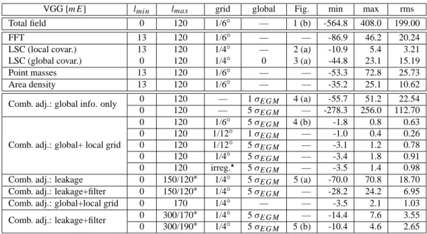
Table 1. Statistical parameters of the vertical gravity gradient deviations [mE] at satellite altitude 250 km applying different continuation

methods to several configurations (confer text), excluding an edge frame of 3◦

VGG [mE] lmin lmax grid global Fig. min max rms

Total field 0 120 1/6◦ — 1 (b) -564.8 408.0 199.00 FFT 13 120 1/6◦ — — -86.9 46.2 20.24 LSC (local covar.) 13 120 1/4◦ — 2 (a) -10.9 5.4 3.21 LSC (global covar.) 0 120 1/4◦ 0 3 (a) -44.8 23.1 15.19 Point masses 13 120 1/6◦ — — -53.3 72.8 25.73 Area density 13 120 1/6◦ — — -35.2 25.1 10.62 0 120 — 1 σEGM 4 (a) -55.7 51.2 22.54

Comb. adj.: global info. only

0 120 — 5 σEGM — -278.3 256.0 112.70

0 120 1/6◦ 5 σEGM 4 (b) -1.8 0.8 0.63

0 120 1/12◦ 1 σEGM — -1.0 0.4 0.26

Comb. adj.: global+ local grid 0 120 1/12◦ 5 σ_EGM — -3.1 1.2 0.78 0 120 1/4◦ 5 σEGM — -3.4 1.8 0.91

0 120 irreg.? 5 σ_EGM — -3.5 1.4 0.98 Comb. adj.: leakage 0 150/120∗ 1/4◦ 5 σ_EGM 5 (a) -70.0 70.8 18.70 Comb. adj.: leakage+filter 0 150/120∗ 1/4◦ 5 σ_EGM — -28.2 24.2 6.95 Comb. adj.: global+local grid 0 170 1/4◦ — — -3.5 2.1 1.03 0 300/170∗ 1/4◦ 5 σEGM — -14.4 7.6 3.55

Comb. adj.: leakage+filter

0 300/190∗ 1/4◦ 5 σEGM 5 (b) -10.4 4.6 2.65 ?_{locations randomly distributed, with a mean distance of 1/4}◦

∗

max. degree of signal / of parameterization

a combination of both approaches suggests itself. Conse-quently, in the next simulation a FFT low pass filtering proce-dure was applied to the test field containing spectral compo-nents up to a maximum degree lmax=150, in order to reduce

the high pass component. Since degree l = 120 corresponds to a spatial wavelength of about 334 km, this value is used as the filter cut-off wavelength. The VGG rms error is reduced from initially 18.7 mE for the unfiltered solution to less than 7 mE, but this gain in accuracy does not suffice for practical calibration/validation purposes, and therefore the additional enhancement of the parameter model has to be envisaged.

Due to the fact that the base functions in Eq. (2) are correlated, in general the normal equation system is full. Therefore, its solution requires enhanced computational ca-pabilities. A parallel computing strategy is applied to solve these large and generally full normal equation systems. In the framework of the project ‘Scientific Supercomputing’ at Graz University of Technology, a parallel computing system based on the Beowulf concept is operable. At the present stage, it is composed of 24 dual-processor (866 MHz) PCs, each with 1 GB RAM and 18 GB local hard disk (Plank, 2001).

In the last case study, such a large system shall be ana-lyzed. The initial gravity signal contains spectral compo-nents up to degree lmax=300, and the parameter model was

enlarged up to degree lmax=190, leading to a normal

equa-tion system of more then 665 million independent elements, corresponding to a memory requirement of about 5.5 GB. A prior low pass filtering of the initial gravity field with a fil-ter cut-off wavelength of 211 km (corresponding to degree

lmax = 190) was applied, and a combined adjustment was

computed, again assuming an accuracy of the global model of 5 σEGM. The rms deviations of the resulting difference

field displayed in Fig. 5b are reduced to 2.65 mE. This con-siderable gain of accuracy proves, that in practice the strategy to enlarge the parameter model, together with a prior filtering of the initial gravity field, is well-suited to reduce the leakage problem.

3.5 Summary and discussion

Table 1 summarizes the major statistical properties of the vertical gravity gradient deviations at a satellite altitude of

h = 250 km related to a variety of case studies, some of them explicitly described in the previous Sects. 3.1 to 3.4, reducing edge effects by excluding an edge frame of 3◦.

From these results it can be concluded that the combined adjustment method is well suited to solve the continuation problem, while all the other strictly local methods discussed in the Sects. 3.1 to 3.3 fail in an adequate representation and thus in a correct continuation particularly of the low fre-quency component. Consequently, the introduction of some kind of trend field information is indispensable to solve the continuation problem.

In Sect. 3.4 it was pointed out, that in practice the most crucial problem will be spectral leakage, because the ini-tial gravity anomaly field can not be perfectly separated into spectral components of low and high degrees l. In fact this problem is of aporetic nature, because if such a perfect har-monic representation would be possible, the whole problem could be solved easily, due to the fact that in this case also

(9)

18 R. Pail : Local gravity field continuation a correct field continuation and field transformation

with-out energy shifts among the spectral components could be performed. The underlying reason for this argumentation is again the bounded definition domain of the gravity data. However, this problem can be considerably reduced by ex-tending the parameter model to sufficiently large degrees

lmax in order to properly represent the initial gravity

infor-mation, in combination with an a priori low pass filtering of the input gravity signal.

At this point it should be emphasized that these simula-tions are based on some very conservative assumpsimula-tions espe-cially concerning the accuracy of the global information and the resolution of the ground gravity data. Even in this case the resulting rms deviations are below the 3 mE-level. How-ever, since the solution strategy applied is a kind of weighted merging of a quite inaccurate global gravity information and the high-accuracy local gravity data, the effects of the rel-ative contributions of these two components – with special concern to the influences on the numerical stability of the corresponding normal equations – will require further analy-sis in the case of larger systems.

An extended version of this paper can be found in Pail (2002).

Acknowledgements. This study was performed in the course of the

GOCE project “From E¨otv¨os to mGal+”, funded by the European Space Agency (ESA) under contract no. 14287/00/NL/DC.

References

Arabelos, D. and Tscherning, C. C.: Support of Spaceborne Gravimetry Data Reduction by Ground Based Data, ESA-Project CIGAR IV, WP 3, Final Report, 95–156, 1996.

Arabelos, D. and Tscherning, C. C.: Calibration of satellite gra-diometer data aided by ground gravity data, J. Geod., 72, 617– 625, 1998.

Cesare: Performance requirements and budgets for the gradiomet-ric mission, Technical Note, GOC-TN-AI-0027, Alenia Spazio, Turin, Italy, 2002.

ESA: Gravity Field and Steady-State Ocean Circulation Mission. Reports for mission selection, The four candidate Earth explorer core missions, SP-1233(1), European Space Agency, 1999. Haagmans, R., de Min, E., and van Gelderen, M.: Fast evaluation

of convolution integrals on the sphere using 1D FFT, and a com-parison with existing methods for Stokes’ integral, Manuscripta Geodaetica, 18, 5, 227–241, 1993.

Heiskanen, W. A. and Moritz, H.: Physical Geodesy, W. H. Free-man and Company, San Francisco, London, 1967.

Koop, R., Visser, P., and Tscherning, C. C.: Aspects of GOCE cal-ibration, in: Proc. International GOCE User Workshop, April 2001, ESA/ESTEC, WPP-188, 51–56, European Space Agency, Noordwijk, 2001.

Lehmann, R.: Gravity field approximation using point masses in free depths, The International Association of Geodesy (IAG), Section IV Bulletin, no. 1, 129–140, 1995.

Lemoine, F. G., Kenyon, S. C., Factor, J. K., Trimmer, R. G., Pavlis, N. K., Chinn, D. S., Cox, C. M., Klosko, S. M., Luthcke, S. B., Torrence, M. H., Wang, Y. M., Williamson, R. G., Pavlis, E. C., Rapp, R. H., and Olson, T. R.: The Development of the Joint NASE GSFC and the National Imagery and Mapping Agency (NIMA) Geopotential Model EGM96, National Aeronautics and Space Administration, Goddard Space Flight Center, Greenbelt, Maryland, 1998.

Pail, R.: Synthetic Global Gravity Model for Planetary Bodies and Applications in Satellite Gravity Gradiometry, Dissertation, Mit-teil. geod¨at. Inst. TU Graz, 85, 135 p., Graz University of Tech-nology, 2000.

Pail, R.: In-orbit calibration and local gravity field continuation problem, ESA-Project “From E¨otv¨os to mGal+”, ESA/ESTEC Contract 14287/00/NL/DC, Final Report, WP 1, 9-112, Euro-pean Space Agency, Noordwijk. (www-geomatics.tu-graz.ac.at/ mggi/research/e2mgp/e2mgp.htm), 2002.

Pail, R., Plank, G., and Schuh, W.-D.: Spatially restricted data dis-tribution on the sphere: the method of orthonormalized functions and applications, J. Geod., 75, 44–56, 2001.

Plank, G.: Implementation of the PCGMA-package on massive par-allel systems, ESA project ‘From E¨otv¨os to mGal+, ESA/ESTEC Contract 14287/00/NL/DC, Final Report, WP 3, 183-216, Euro-pean Space Agency, Noordwijk, 2001.

Rapp, R. H.: Potential coefficient and anomaly degree variance modelling revisited, OSU Rep. no. 2, The Ohio State Univ., Columbus, Ohio, 1979.

Rapp, R., Wang, Y., and Pavlis, N.: The Ohio state 1991 geopo-tential and sea surface topography harmonic coefficient models, OSU Report 410, Department of Geodetic Science and Survey-ing, The Ohio State University, Columbus, Ohio, 1991. Schwarz, K. P., Sideris, M. G., and Forsberg, R.: The use of FFT

techniques in physical geodesy, Geophys. J. Int., 100, 485–514, 1990.

Tscherning, C. C. and Rapp, R. H.: Closed covariance expressions for gravity anomalies, geoid undulations, and deflections of the vertical implied by anomaly degree variance models, OSU Rep. no. 208, Department of the Geodetic Science and Surveying, The Ohio State Univ., Columbus, Ohio, 1974.

Visser, P., Koop, R., and Klees, R.: Scientific data production qual-ity assessment, ESA-Project “From E¨otv¨os to mGal”, Final Re-port, WP 4.1, 157–176, 2000.

Xia, J., Sprowl, D. R., and Adkins-Heljeson, D.: Correction of to-pographic distortions in potential-field data: A fast and accurate approach, Geophysics, 58, 515–523, 1993.