Evolution of a vortex in a strongly stratified shear flow. Part 2. Numerical simulations

(1)

HAL Id: insu-03025142

https://hal-insu.archives-ouvertes.fr/insu-03025142

Submitted on 26 Nov 2020

HAL is a multi-disciplinary open access

archive for the deposit and dissemination of

sci-entific research documents, whether they are

pub-lished or not. The documents may come from

teaching and research institutions in France or

abroad, or from public or private research centers.

L’archive ouverte pluridisciplinaire HAL, est

destinée au dépôt et à la diffusion de documents

scientifiques de niveau recherche, publiés ou non,

émanant des établissements d’enseignement et de

recherche français ou étrangers, des laboratoires

publics ou privés.

Part 2. Numerical simulations

Paul Billant, Julien Bonnici

To cite this version:

Paul Billant, Julien Bonnici. Evolution of a vortex in a strongly stratified shear flow. Part 2.

Nu-merical simulations. Journal of Fluid Mechanics, Cambridge University Press (CUP), 2020, 893,

�10.1017/jfm.2020.227�. �insu-03025142�

(2)

For Peer Review

This draft was prepared using the LaTeX style file belonging to the Journal of Fluid Mechanics 1

Evolution of a vortex in a strongly stratified

shear flow. Part 2. Numerical simulations.

Paul Billant

1

† and Julien Bonnici

1

1_{LadHyX, CNRS, ´}_{Ecole polytechnique, 91128 Palaiseau Cedex, France}

(Received xx; revised xx; accepted xx)

We conduct direct numerical simulations of an initially vertical Lamb-Oseen vortex in an ambient shear flow varying sinusoidally along the vertical in a stratified fluid. The Froude number Fhand the Reynolds number Re, based on the circulation and radius a0of the

vortex, have been varied in the ranges: 0.16 Fh6 0.5 and 3000 6 Re 6 10000. The shear

flow amplitude ˆUS and vertical wavenumber ˆkz lie in the ranges: 0.026 2⇡a0UˆS/ 6 0.4

and 0.1 6 ˆkza0 6 2⇡. The results are analysed in the light of the asymptotic analyses

performed in part 1.

The vortex is mostly advected in the direction of the shear flow but also in the perpendicular direction owing to the self-induction. The decay of potential vorticity is strongly enhanced in the regions of high shear. The long-wavelength analysis for ˆ

kza0Fh ⌧ 1 predicts very well the deformations of the vortex axis. The evolutions of

the vertical shear of the horizontal velocity of the vortex and of the vertical gradient of the buoyancy at the location of maximum shear are also in good agreement with the asymptotic predictions when ˆkza0Fhis sufficiently small. As predicted by the asymptotic

analysis, the minimum Richardson number never goes below the critical value 1/4 when ˆ

kza0Fh⌧ 1. The numerical simulations show that the shear instability is triggered only

when ˆkza0Fh & 1.6 for sufficiently high buoyancy Reynolds number ReFh2. There is

also a weak dependence of this threshold on the shear flow amplitude. In agreement with the numerical simulations, the long-wavelength analysis predicts that the minimum Richardson number goes below 1/4 when ˆkza0Fh & 1.7 although this is beyond its

expected range of validity. Key words:

1. Introduction

In this paper, we continue the analysis of the evolution of a vortex embedded in a vertically sheared flow in a strongly stratified fluid. The main purpose is to determine the conditions under which the vertical shear can grow sufficiently to lead to the development of the shear instability.

This instability is thought to be an important process for the generation of small scales in stratified flows (Riley & deBruynKops 2003; Laval et al. 2003; Lindborg 2006; Brethouwer et al. 2007). In the case of a columnar counter-rotating vortex pair, Deloncle et al. (2008) and Waite & Smolarkiewicz (2008) have reported that the vertical shear generated by the zigzag instability can lead to the development of the shear instability.

(3)

For Peer Review

2 P. Billant and J. Bonnici

This occurs when the buoyancy Reynolds number Reb = ReFh2 (Re is the classical

Reynolds number and Fh the horizontal Froude number) is above a threshold since the

minimum Richardson number is inversely proportional to Reb (Riley & deBruynKops

2003; Deloncle et al. 2008; Augier & Billant 2011). The subsequent destabilization of the Kelvin-Helmholtz billows leads to small-scale turbulence with spectral characteristics similar to those of randomly forced stratified turbulence (Augier et al. 2012; Waite 2013). However, a counter-rotating vortex pair is a very specific flow. Here, we consider the more generic configuration of a single vortex in an ambient shear flow. Such idealized flow contains two elementary ingredients often at play in stratified flows: an horizontal flow with vertical vorticity embedded in a vertical shear flow. In Bonnici & Billant (2020) (referred to hereinafter as part 1), we have studied such a flow by means of a long-wavelength analysis for kzFh ⌧ 1, where kz = ˆkza0 is the dimensionless vertical

wavenumber of the sinusoidal shear flow. This analysis provides a complete description of the vortex dynamics: the evolution of the vortex axis and angular velocity as well as secondary flows created as the vortex is bent. From these results, we have shown that the minimum Richardson number can not go below the critical value 1/4 when kzFh⌧ 1. In

the present paper, we will conduct DNS of this flow for both small and finite kzFh and

analyse its dynamics in the light of the asymptotic analysis.

The paper is organized as follows. The initial conditions, control parameters, and numerical method are described in _{§2. An overview of two typical simulations is first} given in §3. Then, the long-wavelength analysis is first briefly summarized in §4.1 and its predictions for the deformations of the vortex axis are compared to the numerical simulations in§4.2. We then focus on the evolution of the flow at the vortex center and the mid-vertical level where the vertical shear is maximum (§4.3). Again, the asymptotic analysis is used to rationalize the numerical results. Finally, section§5 concentrates on the evolution of the Richardson number for finite kzFh. Section§6 summarizes and discusses

the results.

2. Formulation of the problem

2.1. Initial conditions and governing equations As in part 1, the initial flow is chosen as

u(x, t = 0) = US+ uv, (2.1)

where USis a sinusoidal shear flow and uva columnar vortex with a Lamb-Oseen profile:

US = USsin(kzz)ex, uv=

1 exp( r2₎

r e✓, (2.2) where (x, y, z) and (r, ✓, z) are cartesian and cylindrical coordinates, respectively. (ex, ey, ez) and (er, e✓, ez) are the associated unit vectors. The horizontal and vertical

velocities in cartesian coordinates are denoted uh= (u, v) and w.

In (2.2), the length and time have been non-dimensionalized by the vortex radius a0

and the turnover time 2⇡a2

0/ of the vortex. The shear amplitude US and wavenumber

kz are therefore non-dimensional: US = ˆUS2⇡a0/ , kz= ˆkza0, where ˆUS and ˆkz are the

corresponding dimensional quantities. The governing equations are the incompressible Navier-Stokes equations under the Boussinesq approximation (see part 1). The Reynolds, Froude and Schmidt numbers are defined as

Re =

2⇡⌫, Fh=2⇡a2 0N

, Sc = ⌫

, (2.3)

(4)

For Peer Review

Evolution of a vortex in a strongly stratified shear flow. Part 2. 3

Fh Re kz US lz nx ny nz t 0.1 6000 ⇡ 0.2 2 512 512 256 0.005 0.1 10000 2 0.2 3.142 512 512 256 0.005 0.1 6000 2 0.4 3.142 512 512 256 0.005 0.5 6000 0.3 0.2 20.94 384 384 448 0.01 0.5 6000 ⇡ 0.2 2 832 832 256 0.005 0.5 6000 3⇡/2 0.2 1.333 832 832 448 0.005 Table 1. Overview of the physical and numerical parameters of some typical simulations. For

all simulations, the horizontal dimensions of the domain are lx= ly= 18.

with ⌫ the viscosity,  the di↵usivity and N the Brunt-Väisälä frequency which is assumed constant.

2.2. Numerical method

The equations are integrated numerically by means of a pseudo-spectral method with periodic boundary conditions and a fourth-order Runge-Kutta time advancement scheme (Deloncle et al. 2008). An elliptic truncation of the top one-third of the modes in each direction is applied. The viscous and di↵usive terms are integrated exactly. The horizontal size of the computational domain is taken large lx = ly = 18 in order to minimize

the e↵ect of the periodic boundary conditions. Periodic boundary conditions are indeed responsible for the presence of image vortices located in the virtual boxes adjacent to the computational domain. The strain field due to these image vortices is proportional to

/(2⇡l2

x) and /(2⇡l2y). Periodic boundary conditions also imply that the net circulation

over the domain should be zero (Pradeep & Hussain 2004; Otheguy et al. 2006). Since a single vortex with a non-zero circulation is simulated here, a small background uniform vertical vorticity /(lxly) is therefore artificially present.

Although these two artifacts could be suppressed by implementing the method pro-posed by Rennich & Lele (1997), we have chosen to minimize them by simply taking a large box. Several tests with larger boxes (Bonnici 2018) have shown that setting lx = ly = 18 gives results almost independent of the box size while being not too

computationally expensive. The vertical size is set to lz = 2⇡/kz, so that a single

wavelength of the shear flow is simulated.

Table 1 lists the parameters of some typical simulations. The number of grid points in the x and y directions have been varied from nx= ny= 384 to nx= ny = 832 depending

on the values of the Reynolds and Froude numbers. The number of grid points in the vertical direction ranges from nz= 256 to nz= 448 depending on the values of kz, Re and

Fh. Typically, a high resolution is required for the parameters where the shear instability

develops because it generates small billows while a moderate resolution is sufficient for the other cases. When kz increases, the horizontal and vertical resolutions have to be

increased also since the vertical gradients are larger. The accuracy of the results has been checked by increasing the resolution or the domain horizontal sizes in several runs. The time step varies from t = 0.0025 to t = 0.01. All the numerical simulations have been carried out for Sc = 1. The Froude number has been always kept below unity so as to remain in the strongly stratified regime. The shear amplitude US is also always

kept below unity meaning that the vortex is stronger than the shear flow. The vertical wavenumber has been varied in the range 0.16 kz6 2⇡. The Reynolds number has been

(5)

For Peer Review

3. Overview of the dynamics

3.1. Qualitative description

We first begin by a description of two di↵erent simulations in order to give an overview of the flow dynamics.

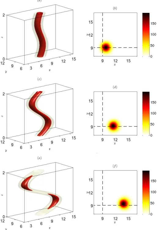
Figures 1 and 2 display the potential vorticity ⇧ = !·⇥rb + 1/F2

hez⇤, where ! is

the vorticity and b the buoyancy, at di↵erent times for kz= ⇡, Fh= 0.1 and kz = 3⇡/2,

Fh = 0.5, respectively, whereas US and Re are fixed to US = 0.2 and Re = 6000.

The first column shows three-dimensional contours while the second column represents a corresponding horizontal cross-section at the vertical level z = lz/4. The vortex is

mostly displaced in the direction of the shear flow, but also slightly in the perpendicular direction as seen in the horizontal cross-sections. Hence, the vertical plane containing the vortex axis is actually oblique relative to the (x, z) plane. The displacement in the y direction is weaker in figure 1 than in figure 2.

A common feature of both simulations is that the potential vorticity decreases faster in the regions of high shear z = 0, lz/2 than in the regions of weak shear z = lz/4, 3lz/4

(figures 1e, 2e,g). Thus, the vortex seems to be torn apart into two separate pancake vortices at large times.

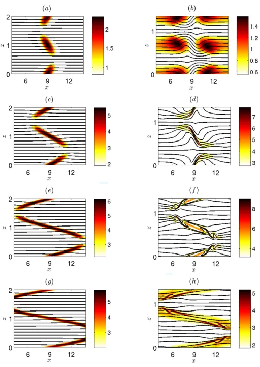
Figure 3 displays the corresponding total vertical shear of the horizontal velocitypSz=

p

(@u/@z)2_{+ (@v/@z)}2_{(color) in the vertical cross-section at y = 9, i.e. passing through}

the vortex center at t = 0. The superimposed black lines show the total density ⇢t =

(⇢0/g)(b + z/Fh2), where ⇢0 is the reference density and g the gravity. For kz = ⇡,

Fh= 0.1 (left column of figure 3), the shear is maximum in the vortex core at the point

xc= 9, zc= 0, lz/2 (note that these coordinates correspond to those of the computational

domain where the vortex center is initially in the middle x = 9, y = 9). As the vortex is progressively bent, pSz grows monotonically with time and becomes rapidly much

higher than the maximum ambient shear max (pS¯z) = kzUS ' 0.6 (figure 3a,c,e,g). The

iso-density lines remain nearly flat since the stratification is strong for this case. Figure 4a shows that the minimum of the Richardson number (black solid line)

Ri = 1 F2 h + @b @z Sz (3.1) decreases with time from min(Ri) = 1/(FhkzUS)2= 253 at t = 0 down to min (Ri) = 3.7

at t = 22 and then slowly re-increases. The quantity min (Ri) thus remains well above the critical value 1/4 necessary for the development of the shear instability of a steady parallel inviscid shear flow (Miles 1961; Howard 1961).

For kz= 3⇡/2, Fh= 0.5 (right column of figure 3), the growth of the maximum shear

p

Szis not monotonic. There is a first stage where the shear is very weak within the vortex

core (see figure 3b at t = 4), i.e. the response of the vortex tends to cancel the ambient shear. Then, the vortex becomes tilted as for kz= ⇡, Fh= 0.1, and the maximum shear is

encountered in the vicinity of xc= 9, zc= 0, lz/2 (figure 3d ) with values approximately

ten times larger than the ambient maximum shear max (pS¯z) ' 0.9. The regions of

high shear are remarkably thin. Later on, the flow strongly dissipates in these regions and the shear becomes maximum at points away from (xc, zc) (figure 3f,h). During this

evolution, the iso-density lines are strongly deformed in contrast to kz = ⇡, Fh = 0.1.

Some overturns can even be seen at some locations at t = 26 (figure 3f ). As seen in figure 4a, the minimum Richardson number for this simulation (grey solid line) decreases from min(Ri) = 1/(FhhzUS)2= 4.5 at t = 0 to a value below Ric = 0.25 for 116 t 6 37. The

(y, z) cross-section at x = 9 of the buoyancy at t = 26 (figure 4c) confirms the presence

(6)

For Peer Review

Figure 1. (Colour online) Left column: three-dimensional contours of the potential vorticity at di↵erent times for Fh = 0.1, kz = ⇡, US = 0.2 and Re = 6000. Right column: corresponding

horizontal cross-sections in the plane z = lz/4 where the advection is the most intense. The

times shown are (a,b) t = 4, (c,d ) t = 13, (e,f ) t = 26. In (a,c,e), the isocontours correspond to 20% (light grey or yellow) and 60% (dark grey or red) of the initial maximum value.

(7)

For Peer Review

Figure 2. (Colour online) Same as figure 1 except that Fh= 0.5, kz= 3⇡/2. The times shown

(8)

For Peer Review

Figure 3. (Colour online) Vertical cross-sections of the shear pSz (color) and of the total

density ⇢t (black contour lines) in the plane y = 9, for Fh = 0.1, kz = ⇡ (left column) and

Fh= 0.5, kz = 3⇡/2 (right column), for US = 0.2 and Re = 6000. The times shown are (a,b)

t = 4, (c,d ) t = 13, (e,f ) t = 26, (g,h) t = 36.

of Kelvin-Helmholtz billows near zc = 0, lz/2. In contrast, no billows can be seen in

these regions in the corresponding (x, z) cross-section at y = 9 (figure 4b). This means that the axes of the Kelvin-Helmholtz billows are mostly oriented in the x direction, i.e. they are parallel to the direction of the ambient shear flow. The black contours in figure 4 delineate the regions where Ri < 0.25. In addition to the unstable regions near

(9)

For Peer Review

0 10 20 30 40 50 t 0 2 4 6 8 mi n ( Ri ) (a)

Figure 4. (Colour online) (a) Minimum Richardson number as a function of time for US= 0.2,

Re = 6000, and Fh= 0.1, kz = ⇡ (black solid line) and Fh= 0.5, kz = 3⇡/2 (grey solid line)

from the DNS. The horizontal black dash-dotted line shows the critical value Ri = 0.25. (b,c) Vertical cross-sections of the buoyancy b at t = 26 in the planes y = 9 (b) and x = 9 (c) for Fh= 0.5, kz = 3⇡/2, US = 0.2, and Re = 6000. The black contours represent the lines where

Ri = 0.25.

(xc, zc), there exist also other unstable regions above and below each pancake vortex at

z = lz/4 and z = 3lz/4 as seen in the (x, z) cross-section (figure 4b). We can also see

some billows and overturns in these regions (figures 4b and 3f ) but in this case, their axes are perpendicular to the direction of the ambient shear. When they occur, these unstable regions appear only in a second stage after those near (xc, zc).

3.2. Time evolution of the vertical shear at the center

For kz = ⇡, Fh = 0.1, the Richardson number is always minimum at the center

point (xc = 9, yc = 9, zc = lz/2) and at the symmetric point (xc = 9, yc = 9, zc = 0).

For kz = 3⇡/2, Fh = 0.5, the Kelvin-Helmholtz instability also develops first at these

points. It is therefore interesting to investigate the evolution of the vertical shear at these locations.

To this end, we first decompose the flow into a mean flow varying only along the vertical and with time ¯u(z, t) and a complementary flow u⇤_:

u = ¯u + u⇤, (3.2) where the overbar denotes the horizontal average over the computational domain, which for any quantity q is defined as

¯ q = 1 lxly Z ly 0 Z lx 0 q(x, y, z, t)dxdy. (3.3) At t = 0, we have ¯u = US and u⇤= uv so that ¯u and u⇤will be called ”shear flow” and

”vortex flow”, respectively.

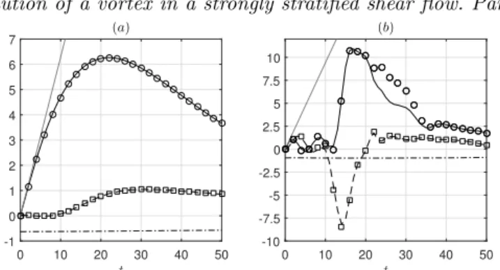
Figure 5a shows the evolution of the di↵erent shear components @ ¯u/@z, @u⇤_{/@z, and}

@v⇤_{/@z at the center (x}

c = 9, yc = 9, zc = lz/2) for Fh = 0.1, kz = ⇡, US = 0.2 and

Re = 6000. The quantity @¯v/@z is always equal to zero at the center and is not plotted. More generally, @¯v/@z always remains very small at any vertical position compared to

(10)

For Peer Review

t 0 10 20 30 40 50 -1 0 1 2 3 4 5 6 7 (a) t 0 10 20 30 40 50 -10 -7.5 -5 -2.5 0 2.5 5 7.5 10 (b)

Figure 5. Time evolution of @ ¯u/@z (black dash-dotted lines), @u⇤/@z (black dashed lines), and @v⇤/@z (black solid lines) at the vortex center xc= 9, yc= 9, zc= lz/2 for (a) Fh= 0.1, kz= ⇡,

and (b) Fh = 0.5, kz = 3⇡/2 for US = 0.2 and Re = 6000. The straight grey lines represent

the relation kzUSt. The symbols show the horizontal vorticity components !x⇤(circles) and !⇤y

(squares).

@ ¯u/@z. We see that the mean shear @ ¯u/@z (dash-dotted line) remains almost constant and equal to kzUS = 0.63. In contrast, the shear component @v⇤/@z (solid line) grows

first linearly and then saturates at t_{' 22 at the value @v}⇤_{/@z = 6.3, i.e. ten times the}

ambient shear _{|@ ¯u/@z|. The other component @u}⇤_{/@z remains very weak up to t = 10}

and then increases up to @u⇤_/@z _{' 1 at t = 30. This quantity therefore saturates at a}

lower value and later than its counterpart @v⇤_/@z.

The initial behaviour of the vertical shear of the vortex @u⇤_{/@z and @v}⇤_{/@z can be}

simply understood by considering that the vortex is displaced at the velocity U (z) in the x direction, i.e. uv(x U t, y), as assumed by Lilly (1983). This gives:

@uv @z = dU dzt @uv @x . (3.4) Since uv = ( ⌦y, ⌦x), where ⌦(r) is the angular velocity of the vortex, we have

@vv/@x = ⌦ = 1 and @uv/@x = 0 at the center r = 0. Thus, (3.4) yields

@uv

@z = 0, @vv

@z = kzUSt, (3.5) at z = lz/2. The straight grey line in figure 5a confirms that @v⇤/@z increases initially

at the rate kzUSt. This also explains why @u⇤/@z remains very small initially. The

subsequent evolutions will be explained later thanks to the asymptotic analysis performed in part 1.

In figure 5a, we have also plotted with symbols the horizontal vorticity components !⇤

x and !y⇤ where !⇤ =r ⇥ u⇤. They are nearly superposed to @v⇤/@z and @u⇤/@z,

respectively, because the vertical velocity is very small compared to the horizontal velocity. In other words, !⇤

x' @v⇤/@z and !⇤y' @u⇤/@z.

Similarly, figure 5b displays the time evolution of @ ¯u/@z, @u⇤_{/@z, and @v}⇤_{/@z at the}

center point for Fh= 0.5 and kz= 3⇡/2, still for US = 0.2 and Re = 6000. In contrast to

the case Fh= 0.1, kz= ⇡ (figure 5a), @v⇤/@z follows the relation (3.5) only at the very

beginning t. 2. Instead, both shear components @u⇤_{/@z and @v}⇤_{/@z first oscillate with}

a phase lag and with a period around 2⇡, i.e. the period corresponding to the angular velocity on the vortex axis ⌦ = 1. Because of these oscillations, we can notice that @v⇤_{/@z goes back to zero around t}_{' 4} _{5 while @u}⇤_{/@z is approximately opposite to}

@ ¯u/@z. Thus, the total shear Sz is weak at the center as already observed in figure 3b at

(11)

For Peer Review

t 0 10 20 30 40 50 0 1 2 3 4 5 6 7 8 9 (a) t 0 10 20 30 40 50 0 1 2 3 4 5 6 7 8 9 (b)

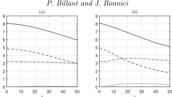
Figure 6. Time evolutions of the global kinetic energy ¯Ek+ Ekh⇤ + Ekz⇤ (black solid line), the

mean flow kinetic energy ¯Ek (black dash-dotted line), the vortex horizontal kinetic energy E⇤kh

(black dashed line), the vortex vertical kinetic energy E⇤

kz (grey dashed line) and the potential

energy Ep(grey solid line) for (a) Fh= 0.1, kz = ⇡ and (b) Fh= 0.5, kz= 3⇡/2 for US= 0.2,

Re = 6000.

Then, @u⇤/@z and @v⇤/@z are both abruptly amplified up to an absolute value around 10. Remarkably, @u⇤/@z becomes now negative and saturates earlier than @v⇤/@z. Later on, |@u⇤_/@z_{| decreases very quickly while |@v}⇤_/@z_{| decays more slowly. The vorticity}

components !⇤

x and !⇤y have been also plotted in figure 5b. They are again almost

identical to @v⇤_{/@z and @u}⇤_{/@z except} _!⇤

x for 21 6 t 6 35. This corresponds to the

time interval when the Kelvin-Helmholtz billows exist. They produce a finite vertical velocity w⇤_{, making the term @w}⇤_{/@y in !}⇤

x no longer negligible. In contrast, the term

@w⇤_{/@x is still negligible in !}⇤

y, most probably because the axes of the Kelvin-Helmholtz

billows are aligned with the x direction.

3.3. Global energy and enstrophy evolutions

Figure 6 presents the evolutions of the energies integrated over the whole computational domain for the two simulations for kz= ⇡, Fh= 0.1, and kz= 3⇡/2, Fh= 0.5, previously

described. The kinetic energies have been decomposed into a mean part and a vortex part using the decomposition (3.2):

¯ Ek = 1 lz Z V ¯ u2 2 dV , E ⇤ kh= 1 lz Z V u⇤ h 2 2 dV , E ⇤ kz= 1 lz Z V w⇤2 2 dV , (3.6) where E⇤

kh and E⇤kz are the horizontal and vertical kinetic energies of the vortex part.

The integral over the computational domain V is divided by lz in order to enable the

comparisons between simulations carried out with distinct vertical wavelengths (Note that we do not divide by V in order to be able to compare simulations with di↵erent horizontal domain sizes). Similarly, the global potential energy per vertical length unit is: Ep= 1 lz Z V F2 hb2 2 dV . (3.7) The kinetic energy of the mean flow ¯Ek (black dash-dotted lines) remains approximately

constant even if it increases slightly at the beginning for kz = 3⇡/2, Fh= 0.5 (figure 6b).

In contrast, the horizontal kinetic energy of the vortex E⇤

kh(black dashed lines) decreases

regularly following an approximately linear trend. The vertical kinetic energy E⇤ kz (grey

dashed lines) and the potential energy Ep (grey solid lines) remain always very weak

compared to the horizontal kinetic energy.

Likewise, figure 7 displays the evolutions of the global enstrophies per vertical length

(12)

For Peer Review

t 0 10 20 30 40 50 0 25 50 75 100 125 150 175 (b) t 0 10 20 30 40 50 60 0 25 50 75 100 125 150 (a)

Figure 7. Time evolutions of the global total enstrophy ¯Z +Zh⇤+Zz⇤(black solid line), the mean

flow enstrophy ¯Z (black dash-dotted line), the vortex horizontal enstrophy Zh⇤ (black dashed

line) and the vortex vertical enstrophy Z⇤

z (grey dashed line) for (a) Fh= 0.1, kz= ⇡ and (b)

Fh= 0.5, kz= 3⇡/2 for US= 0.2, Re = 6000.

unit, decomposed using (3.2): ¯ Z = 1 lz Z V ¯ !2 2 dV , Z ⇤ h= 1 lz Z V !⇤h 2 2 dV , Z ⇤ z = 1 lz Z V ⇣⇤2 2 dV , (3.8) where ¯! is the vorticity of the shear flow and !⇤h and ⇣⇤ the horizontal and vertical

vorticities of the vortex part. The global horizontal enstrophy of the vortex Zh⇤ (black

dashed lines) increases and then decreases while its vertical counterpart Zz⇤(grey dashed

lines) continuously decays. Remarkably, the growth of Zh⇤ is much more pronounced for

kz= ⇡, Fh= 0.1 than for kz = 3⇡/2, Fh = 0.5 although the vertical wavenumber kz is

higher in this second case. The enstrophy of the mean shear ¯Z remains approximately constant like the mean kinetic energy ¯Ek. Since the mean enstrophy ¯Z for kz= 3⇡/2 is

more than twice the one for kz= ⇡, the maximum of the total enstrophy (solid lines) is

comparable in the two simulations even if max (Z⇤

h) is lower for kz= 3⇡/2.

4. Comparison to the long-wavelength asymptotic analysis

4.1. Reminder

In part 1, we have performed a long-wavelength asymptotic analysis for kzFh⌧ 1, i.e.

for small vertical Froude number Fv = kzFh= /(a0lzN ). Leading order viscous e↵ects

have been also taken into account. This analysis has provided evolution equations for the position of the vortex center at each level z:

x = U (z)t + x(z, t), (4.1) y = y(z, t), (4.2) where @ x @t =  A(z, t) 2 @2 _y @z2 ✓ #(z, t) +@Cw @t (z, t) ◆_d2_U dz2 F 2 h, (4.3) @ y @t =  _@ @z ✓ A(z, t) 2 t dU dz ◆ +A(z, t) 2 @2 _x @z2 + @_Sw @t (z, t) d2_U dz2 F 2 h. (4.4)

where_CwandSware the e↵ects of internal waves excited at t = 0 and that decay quickly

afterwards. The parameters_{A and # correspond to the self-induction of the vortex and} an advection correction, respectively. The expressions of all these parameters are given in part 1.

(13)

For Peer Review

An approximation for the solution of (4.3-4.4) has been found in part 1 in the form x = Fh2  Cw(z, t) + Z t 0 #(z, )d d 2_U dz2, (4.5) y = Fh2  Sw(z, t) d2_U dz2 + Z t 0 @ @z ✓ A(z, ) 2 dU dz ◆ d . (4.6) In addition, the asymptotic analysis has shown that the angular velocity of the vortex evolves according to @⌦ @t =  Fh2t⌦3+ t2 2Re ˜r @⇣0 @ ˜r ✓ dU dz ◆2 , (4.7) where ⇣0= (1/˜r)@ ˜r2⌦/@ ˜r is the vertical vorticity and ˜r is the local radius with respect

to the center of the vortex at the level z: ˜r2_{= (x} _{U (z)t} _x)2_{+ (y} _y)2_{. The first}

term in the right-hand side of (4.7) ensures the conservation of potential vorticity while the second term describes the leading viscous e↵ect. This e↵ect is proportional to t2

because the vertical shear grows like tdU/dz at leading order. Internal waves have been neglected in (4.7) since their e↵ects have been shown to be very weak In part 1, the equation (4.7) has been solved asymptotically. In particular, an analytic expression for the angular velocity on the vortex axis has been obtained:

⌦(˜r = 0, z, t) = q 1

(1 + 2 T3_/3)2_{+ T}2

, (4.8) where T = Fht|dU/dz| and (z) = 1/ ReFh3|dU/dz| . This expression is in very good

agreement with the exact result obtained by numerical integration of (4.7). It will be therefore used in the following.

In addition, the asymptotic analysis has provided the horizontal velocity at order O[(kzFh)2] and the vertical velocity and buoyancy at leading order. They allowed us to

predict the evolution of the vertical shear of the horizontal velocity, the vertical buoyancy gradient and the Richardson number at the vortex center at z = lz/2. These predictions

will be compared to the DNS in section§4.3. Before, we begin by presenting in the next section a comparison between the location of the vortex center observed in the DNS and the asymptotic predictions (4.1)-(4.2).

4.2. Deformations of the vortex axis

In order to estimate the position of the vortex center in the numerical simulations, we have used two methods: one based on the potential vorticity ⇧ and the other on the vertical vorticity ⇣. In each case, the displacements of the vortex center have been estimated from vorticity centroids:

x⇧c (z, t) = hx⇧ih h⇧ih , yc⇧(z, t) = hy⇧ih h⇧ih , (4.9) or x⇣c(z, t) = hx⇣ih h⇣ih , yc⇣(z, t) = hy⇣ih h⇣ih , (4.10) where the brackets denote

h'ih=

Z

'>'c

'dxdy. (4.11)

(14)

For Peer Review

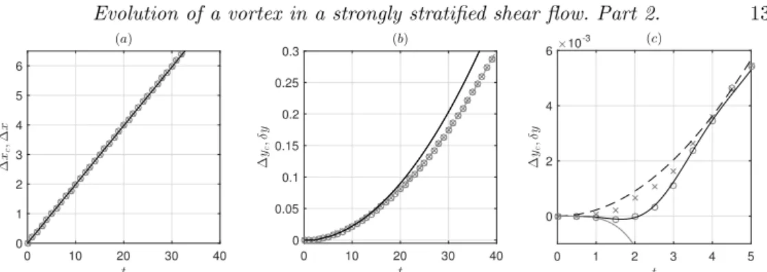
0 10 20 30 40 t 0 1 2 3 4 5 6 ∆ xc ,∆ x (a) 0 10 20 30 40 t 0 0.05 0.1 0.15 0.2 0.25 0.3 ∆ yc , δy (b) 0 1 2 3 4 5 t 0 2 4 6 ∆ yc , δy ×10-3 (c)

Figure 8. (a,b) Comparison between the vertical vorticity centroids x⇣

c and yc⇣ (grey open

circles), the potential vorticity centroids x⇧

c and y⇧c (grey crosses) and the asymptotic

predictions for the displacements x and y (black solid lines) in the plane z = lz/4. (c)

displays a close-up view of the initial evolution of y⇣c (grey open circles), yc⇧ (grey crosses),

and y (black solid line). The asymptotic prediction in the absence of internal waves, i.e. by settingCw =Sw = 0 in (4.5)-(4.6) has been also reported (black dashed line). The short-time

asymptotic prediction for y has been plotted as well (grey solid line). The parameters are Fh= 0.5, kz= 0.3, US= 0.2, and Re = 6000.

The horizontal integration is carried out only in the regions where the vorticity is larger than a critical value ⇧c, ⇣c. In this way, we exclude the small background vorticity due to

the fact that the total vorticity is zero owing to the use of periodic boundary conditions. The values ⇧c = 0.05 maxt=0(⇧) and ⇣c = 0.05 maxt=0(⇣) have been chosen as they

provide results almost independent of the size of the computational domain and the particular values of the thresholds.

The tracking method based on the potential vorticity seems more natural since it is a transported quantity in the inviscid limit. However, we shall see that the method based on the vertical vorticity will enable a closer comparison to the asymptotic results. This is because the condition used to normalize the streamfunction at first order 1 in the

asymptotic analysis:⌦x_r2 h 1↵_h= 0, ⌦yr2h 1↵_h= 0, implies x⇣c = hx⇣ih h⇣ih = ⌦ x[⇣0+ (kzFh)2r2h 1+ ...]↵_h h⇣0+ (kzFh)2r2h 1+ ...i_h = hx⇣0(˜r)ih h⇣0ih = x, (4.12) and, similarly y⇣

c = y, where ( x, y) are the asymptotic displacements (4.1)-(4.2)

and ⇣0is the leading order vertical vorticity.

In the next sections, we compare the asymptotic and numerical results for di↵erent parameters.

4.2.1. In-depth analysis of a simulation

Figure 8 compares the total displacements x = USt + x and y as predicted by

the asymptotics to the positions xc and yc of the vortex estimated from the vertical

vorticity and potential vorticity centroids at the level z = lz/4 for Fh = 0.5, kz = 0.3,

US = 0.2, and Re = 6000. The agreement is excellent at all times for x and up to

t_{' 15 for y. The dominant displacement is in the x direction (figure 8a) and given by} USt while the deviations x and y are much smaller.

The displacement of the vortex estimated from the vertical vorticity, ( x⇣

c, y⇣c), and

from the potential vorticity, ( x⇧

c , yc⇧), are almost equal. However, if we focus on the

initial evolution of y⇣

c and y⇧c (figure 8c), we see that they are actually di↵erent for t6

4. The displacement y⇣

c (crosses) is first slightly negative for t6 2 in excellent agreement

(15)

For Peer Review

0 5 10 15 20 z -10 -5 0 5 10 ∆ x ζ,∆c x (a) 0 5 10 15 20 z -0.3 -0.2 -0.1 0 0.1 0.2 0.3 ∆ y ζ,c δy (b)

Figure 9. (a,b) Comparison between the vertical vorticity centroids x⇣

c (a) and y⇣c (b) (grey

dashed lines with open circles) and the asymptotic predictions for the displacements x and y (black solid lines) as a function of z at di↵erents times t = 6, 12, 18, 24, 30, 36 (increasing amplitudes). The dotted lines represent the exact solution obtained by numerical integration of (4.3-4.4). The parameters are Fh= 0.5, kz= 0.3, US= 0.2, and Re = 6000.

estimated from the potential vorticity y⇧c (open circles) increases monotonically. As

explained above, the estimation of the vortex center from the vertical vorticity is in much better agreement with the asymptotics than the estimation from the potential vorticity because the normalisation condition used in the asymptotic analysis is based on the vertical vorticity.

Nevertheless, if the e↵ects of the internal waves are neglected in (4.5)-(4.6) (i.e. Cw=

Sw = 0), the asymptotic prediction (black dashed line) is then close to yc⇧. This

confirms that internal waves play a key role at the start-up of the flow evolution. Because of these waves, the initial evolution of y at z = lz/4 is of the form y = k2zUS t4, where

= 3.826_{⇥ 10} 3 _{is a constant (part 1), as shown by the grey solid line in figure 8c. In}

contrast, when internal waves are neglected, y evolves initially as y_{/ t}2 _{(black dashed}

line).

Figure 9 shows the vertical profiles of the x and y displacements at di↵erent times. As can be seen in figure 9a, the agreement between the vertical vorticity centroid x⇣ c

measured in the simulations (grey dashed lines with open circles) and the asymptotic prediction x (black solid lines) is excellent along all the vertical. It follows very well the sinusoidal profile x = Ust sin(kzz) since the correction x is much smaller. There is

also a good agreement between the numerics and the asymptotics for the y-displacement (figure 9b) although some departures appear around the extrema for large time, as was already seen in figure 8b. It is also clearly visible that the y-displacement departs from a sinusoidal shape as time increases. This non-sinusoidal profile comes from the vertical variations of the parameter_{A (in the second term of (4.6)) induced by the modulation of} the angular velocity of the vortex along the vertical. We have also plotted in figure 9 the exact asymptotic displacements obtained by numerical integration of (4.3-4.4) (dotted lines). However, these curves are only visible around the maxima of y at the latest time shown (figure 9b) because they are almost identical to the approximation (4.5)-(4.6).

We have also compared the vertical velocity field predicted by the asymptotics against its numerical counterpart. Figure 10 displays horizontal cross-sections of w in the plane z = lz/2 where it is maximum. A very good qualitative and quantitative agreement

is observed even at t = 18 (figures 10c,f ) apart from the existence of small wave-like disturbances in the DNS that are absent in the asymptotics. The close agreement between the asymptotic and numerical results can be further seen in the temporal variations of the

(16)

For Peer Review

Figure 10. (Colour online) Horizontal cross sections in the plane z = lz/2 of (a,b,c) the vertical

velocity calculated asymptotically and (d,e,f ) in the DNS for Fh= 0.5, kz = 0.3, US= 0.2, and

Re = 6000 at t = 2 (a,d ), t = 6 (b,e) and t = 18 (c,f ).

0 10 20 30 40 t 0 0.02 0.04 0.06 0.08 0.1 wm (a) 0 10 20 30 40 t 0 0.005 0.01 0.015 wm (b) 0 2 4 6 8 0 0.005 0.01 0 10 20 30 40 t 0 1 2 3 4 5 6 7 wm ×10-3 (c) 0 5 10 0 1 2 3 ×10 -3

Figure 11. Evolution of the maximum velocity wm in the plane z = lz/2 in the DNS (grey

dashed lines) and from the asymptotic predictions (black solid lines) for Re = 6000, US = 0.2

for (a) Fh= 0.5, kz = 0.3, (b) Fh= 0.1, kz = 1.5, (c) Fh= 0.1, kz = 0.3. The insets in (b,c)

display a close-up view of the initial evolution.

maximum values of w and b (figures 11a and 12a ). The asymptotic and numerical results begin to slightly depart from each other as late as t ' 10. The maximum values of w and b increase initially linearly and then saturate with oscillations superimposed. These oscillations are due to the internal waves excited at t = 0. Two periods T = 2⇡Fh = ⇡

and T = 2⇡/⌦(r = 0) = 2⇡ are mixed explaining why the oscillations look somewhat irregular, especially for wm(figure 11a).

Similar agreements have been observed for di↵erent values of US and Re. In the next

subsection, we investigate the e↵ects of varying the Froude number and the wavenumber. 4.2.2. E↵ects of Fh and kz

Figures 11b,c and 12b,c show the evolution of the maximum vertical velocity and buoyancy for a lower Froude number Fh = 0.1 and two di↵erent wavenumbers. In the

first case (figures 11b and 12b), the wavenumber has been increased to kz= 1.5 so that

the product kzFh= 0.15 is the same as before while, in the second case (figures 11c and

12c), the wavenumber is still kz = 0.3. The agreement is good for both wavenumbers

(17)

For Peer Review

0 10 20 30 40 t 0 0.1 0.2 0.3 0.4 0.5 0.6 bm (a) 0 10 20 30 40 t 0 0.5 1 1.5 2 2.5 bm (b) 0 10 20 30 40 t 0 0.2 0.4 0.6 0.8 1 bm (c)

Figure 12. Evolution of the maximum buoyancy bm in the plane z = lz/2 in the DNS (grey

dashed lines) and from the asymptotic predictions (black solid lines) for Re = 6000, US = 0.2

for (a) Fh= 0.5, kz= 0.3, (b) Fh= 0.1, kz= 1.5, (c) Fh= 0.1, kz= 0.3.

that the oscillations of the maximum buoyancy are strongly reduced when Fh = 0.1

(figure 12b,c) compared to Fh= 0.5 (figure 12a). This is because the amplitude of the

internal waves in the buoyancy scales as the Froude number. In contrast, oscillations are still visible in the evolution of the maximum asymptotic vertical velocity for Fh = 0.1

(figures 11b,c) since the amplitude of the internal waves in this field does not vanish in the limit of small Froude number. However, no oscillations are present at large time in the DNS (dashed lines) for Fh = 0.1 unlike for Fh = 0.5 (figure 11). Nevertheless, the

mean evolution of wm in the DNS is close to the one predicted by the asymptotics for

Fh = 0.1. The insets in figures 11b,c show a close-up view of the initial evolution of

wm for Fh = 0.1. We can see that the oscillations are quickly damped in the DNS for

kz= 1.5 (figure 11b) and disappears for t& 3. For kz= 0.3 (figure 11c), they persist for

a longer time and start to decay only after t _{⇠ 10. Before, the agreement between the} asymptotics and the numerics is excellent.

The reason for these discrepancies is the following. As already mentioned, the asymp-totic problem has been solved in part 1 for long-wavelength by assuming kzFh ⌧ 1.

The reason why kzFh is the appropriate parameter is that the buoyancy lengthscale is

the natural vertical lengthscale of vortical motions in strongly stratified inviscid flows (Billant & Chomaz 2001). However, this self-similarity does not apply to the internal waves that are generated at the start-up of the motion because they evolve on the fast time scale 1/Fh and not on the turnover timescale of the vortex. For this reason, the

asymptotic calculation of the internal waves component performed in part 1 is actually correct only when kz is small but not if kz is of order unity and Fhsmall. For finite kz,

the internal waves could be computed only numerically. However, the inset in figure 11b shows that only few oscillation cycles are present at the beginning. This is because the internal waves quickly propagate away from the vortex core. Indeed, their radial group velocity, which is proportional to k2

z/Fh, is large for kz= O(1) and Fh⌧ 1. In contrast,

when kzis small and Fhfinite, the radial group velocity is small meaning that the internal

waves remain a long time in the vortex core, i.e. are almost purely standing waves as found in the asymptotic analysis. This is the reason why the oscillation cycles are seen for a longer time for kz= 0.3 (inset in figure 11c) than for kz= 1.5 (inset in figure 11b).

Since finite kzwill be mostly considered in the following, we have chosen to completely

neglect the internal waves for these reasons.

4.3. Evolution of the vertical shear and the Richardson number

We now investigate the evolution of the flow at the vortex center and at the level z = lz/2 where the ambient shear is maximum. As seen in section§3, this is the location

(18)

For Peer Review

0 15 30 45 60 t 0 2 4 6 ∂ u ∗/c ∂ z , ∂ v ∗/c ∂ z (a) 0 15 30 45 60 t 0 10 20 30 40 50 ∂ bc / ∂ z (b) 0 15 30 45 60 t 0 2 4 6 8 10 Ri c (c)

Figure 13. Evolution of (a) @u⇤_{/@z (dashed line), @v}⇤_{/@z (solid line), (b) @b/@z and (c) Ri}

at ˜r = 0, z = lz/2 from the DNS (grey lines) and predicted from the asymptotics (black lines).

The parameters are Fh= 0.1, kz= ⇡, US= 0.2, Re = 6000.

(together with the symmetric point z = 0) where the Richardson number reaches its minimum or where the Kelvin-Helmholtz instability first appears.

Figures 13a,b compare @u⇤/@z, @v⇤/@z and @b/@z at the vortex center at z = lz/2

observed in the DNS for Fh = 0.1, kz = ⇡, US = 0.2, and Re = 6000 (grey lines) to

their asymptotic counterparts derived in part 1 (black lines). Apart from @u⇤

c/@z, the

agreement is very good over the entire time range investigated. Since @v⇤

c/@z and @bc/@z

depend only on the quantity t⌦cat leading order in kzFh(where ⌦cis the angular velocity

at ˜r = 0, z = lz/2), this agreement is an indirect confirmation of the relation (4.8) for

the angular velocity at the vortex center. The magnitude of @u⇤

c/@z is much lower than

for @v⇤

c/@z. The beginning of its evolution is well predicted by the asymptotics until

t_{' 5} 10 but not later. Several checks led us to the conclusion that this discrepancy is not due an error in our calculations but is most probably due to higher order e↵ects, not considered in the asymptotic analysis, that become quickly dominant over the leading order when kzFhUSt > 1. This is because the asymptotic expansion is not uniformly

asymptotic in time since the long-wavelength assumption is expected to be no longer valid when kzFhUSt > 1 because vertical gradients grow like kzUSt. Nevertheless, figures

13a,b show that the asymptotics for @vc⇤/@z and @bc/@z remain in good agreement even

when t = 60, i.e. kzFhUSt ⇠ 4. Despite this discrepancy on @u⇤c/@z, figure 13c shows

that the asymptotic Richardson number Ricis in good agreement with the one computed

from the DNS since @u⇤

c/@z is one order smaller in (kzFh)2 than @vc⇤/@z and @bc/@z.

The main assumption of the long-wavelength asymptotic analysis, i.e. kzFh ⌧ 1, is

reasonably well satisfied for the parameters of figure 13 since kzFh = 0.31. Figure 14

further compares the evolutions of @u⇤

c/@z, @v⇤c/@z, @bc/@z and Ric when Fh or kz are

increased. Surprisingly, the agreement between the asymptotics and numerics for @v⇤c/@z

and @bc/@z remains satisfactory even if kzFh has been increased up to unity. Regarding

@u⇤c/@z (figure 14a), a large discrepancy is always observed like in figure 13a. When Fh

is increased from Fh = 0.1 (dashed-dotted lines) to Fh = 0.5 (solid lines), keeping the

wavenumber constant kz = 2, @v⇤c/@z and @bc/@z decrease (figure 14b,c) while @u⇤c/@z

increases (figure 14a). The maxima of @u⇤c/@z and @v⇤c/@z become even of the same

magnitude for Fh = 0.5 in sharp contrast to what was observed in figure 13. Large

oscillations are present in the DNS for Fh= 0.5 (figure 14). We have checked that they

are not due to the internal waves that have been neglected in the asymptotics. They seem rather related to some vortex waves since @u⇤

c/@z and @v⇤c/@z oscillate out of phase as

also observed in figure 5b.

(19)

For Peer Review

0 10 20 30 40 50 t 0 1 2 3 ∂ u ∗/c ∂ z (a) 0 10 20 30 40 50 t 0 1 2 3 4 5 6 7 8 ∂ v ∗/c ∂ z (b) 0 10 20 30 40 50 t 0 10 20 30 40 50 60 ∂ bc / ∂ z (c) 0 10 20 30 40 50 t 0 2 4 6 8 10 Ri c (d)

Figure 14. Evolution of (a) @u⇤/@z, (b) @v⇤/@z, (c) @b/@z and (d ) Ri at ˜r = 0, z = lz/2, for

US = 0.2, Re = 6000, for (Fh= 0.1, kz = 2) (dash-dotted lines), (Fh= 0.25, kz = 2) (dashed

lines), (Fh= 0.5, kz = 2) (solid lines) and (Fh= 0.1, kz= 5) (dotted lines) from the DNS (grey

lines) and predicted by the asymptotics (black lines).

kz = 5 (dotted lines) keeping the Froude number constant Fh = 0.1, the vertical shear

and the buoyancy vertical gradient saturate earlier and at higher levels.

The minimum of the Richardson number decreases as kz or Fhincreases (figure 14d ).

The asymptotic and numerical Richardson number remains in rough agreement even for Fh= 0.5 (solid lines) despite the large increase of @u⇤c/@z as Fh increases. In particular,

the minimum values are min(Ric)' 0.95 and min(Ric)' 0.6, respectively. The minimum

of the asymptotic Richardson number is lower than the bound min(Ric) > 3.43 derived

in part 1 for kzFh ⌧ 1 since kzFh = O(1). We can notice that the beginning of the

evolution of the Richardson number for (Fh = 0.25, kz= 2) (dashed lines) is similar to

the one for (Fh= 0.1, kz= 5) (dotted lines) (figure 14d ) since kzFh= 0.5 in both cases.

The subsequent evolutions di↵er because the buoyancy Reynolds numbers are di↵erent: Reb = 1500 and Reb= 60, respectively.

Similar agreements have been observed for other values of US and Re.

5. Evolution of the Richardson number for finite k

z

F

h

In this section, we now study the regime of finite kzFh mainly based on the DNS since

the long-wavelength analysis is a priori no longer expected to be valid. Figure 15a displays the evolution of the Richardson number in the DNS at the vortex center at z = lz/2 for

(20)

For Peer Review

0 10 20 30 40 t 0 1 2 3 4 5 Ri c (a) 0 5 10 15 USt 0 1 2 3 4 5 Ri c (b) 0 10 20 30 40 t 0 1 2 3 4 5 Ri c (c)

Figure 15. Evolution of the Richardson number at the vortex center at z = lz/2 for US= 0.2

and for (a) kz = ⇡/2, Fh = 0.5, Re = 1500 (solid line), kz = ⇡/2, Fh = 0.5, Re = 6000

(dash-dotted line), kz = ⇡, Fh= 0.25, Re = 6000 (dashed line), kz = ⇡, Fh= 0.5, Re = 6000

(dotted line). (b) Ric as a function of USt for Re = 6000, kz = ⇡, Fh = 0.5 and US = 0.2

(solid line), US= 0.3 (dash-dotted line) and US = 0.4 (dashed line). (c) Ricas a function of t

for kz = ⇡, Fh= 0.5, US = 0.2 and Re = 6000 (solid line), Re = 5000 (dash-dotted line) and

Re = 4000 (dashed line).

four particular combinations of the parameters (kz, Fh, Re). It is interesting to compare

two curves at a time. First, the solid and dashed lines correspond to di↵erent Froude numbers Fh= 0.5 and Fh= 0.25, respectively, but with the same values of the rescaled

wavenumber kzFh= ⇡/4 and of the buoyancy Reynolds number ReFh2= 375. These two

curves superpose quite well apart from the oscillations. Similarly, the dashed and dashed dotted lines share the same values of kzFh = ⇡/4 and of Reynolds number Re = 6000

but have di↵erent buoyancy Reynolds number. In this case, the evolutions of Ric di↵er.

Finally, the dashed and dotted lines have the same wavenumber kz = ⇡ and Reynolds

number Re = 6000 but di↵erent Froude numbers. In this case also, the evolution of Ric

di↵ers widely as already seen before in figure 14. Altogether, this demonstrates that Ric

depends mainly on (kz, Fh, Re) only through the two parameters kzFh and ReFh2. The

same conclusion can be drawn from other sets of parameters.

Similarly, figure 15b shows the evolution of Ric for di↵erent values of US for kz= ⇡,

Fh= 0.5, Re = 6000. The time has been rescaled by US in this case. The di↵erent curves

are very close to each other, indicating that US has only a weak e↵ect on the Richardson

number. Finally, figure 15c shows that the Reynolds number has only a small influence on the evolution of Ric when it is sufficiently large and when the other parameters are

kept constant.

The minimum value of the Richardson number min(Ric) reached in most of the DNS

is further summarized in figure 16 as a function of the three main parameters: kzFh,

US and ReFh2. A filled symbol is used when the shear instability is observed and an

open symbol, otherwise. When the shear instability develops, the minimum Richardson number is then generally negative owing to the overturnings induced by the instability. However, this negative value has no particular meaning except the fact that it is below the threshold 1/4. As seen in figure 16a, min(Ric) decreases with kzFh and goes below 1/4

when kzFh& 1.6 for both Fh = 0.25 (diamonds) and Fh = 0.5 (circles) for Re = 6000.

However, the shear instability has been observed only for Fh = 0.5. For Fh = 0.25,

the minimum Richardson number is just below 1/4: min(Ric) = 0.2 for the highest

wavenumber that has been investigated kzFh= 1.6. It is likely that the shear instability

would be also triggered for Fh= 0.25 if a larger value of kzFhwere investigated. As shown

previously, the di↵erences between the minimum Richardson number for Fh= 0.25 and

(21)

For Peer Review

0 0.5 1 1.5 2 2.5 kzFh -0.5 0 0.5 1 1.5 2 2.5 3 3.5 mi n ( Ri c ) (a) 0.2 0.3 0.4 US -0.2 0 0.2 0.4 0.6 0.8 1 mi n ( Ri c ) (b) 300 800 1300 1800 ReF_h2 0 0.5 1 1.5 mi n ( Ri c ) (c)

Figure 16. Minimum Richardson number in numerical simulations (symbols) at the vortex center at z = lz/2) as a function of (a) kzFh, (b) USand (c) ReFh2. The di↵erent symbols/lines

correspond to, (a): Fh= 0.5, Re = 6000 (circles), Fh= 0.25, Re = 6000 (diamonds), Fh= 0.5,

Re = 1500 (plus sign) for US = 0.2, ; (b): Fhkz = ⇡/4 (downward triangle), Fhkz = ⇡/2

(circles), Fhkz = 3⇡/4 (squares) and Fhkz = ⇡ (upward triangle) for Fh = 0.5, Re = 6000;

(c): Fhkz = ⇡/4, Fh = 0.5 (downward triangle), Fhkz = ⇡/4, Fh= 0.25 (cross), Fhkz = ⇡/2,

Fh= 0.5 (circles), Fhkz = ⇡/2, Fh= 0.25 (diamonds) and Fhkz= 3⇡/4, Fh= 0.5 (squares) for

US = 0.2. Filled and empty symbols correspond to runs where the shear instability develop or

not, respectively. The grey lines in (a) represent the asymptotic predictions for Fh= 0.5 (solid

line) and Fh = 0.25 (dashed line) for Re = 6000, US = 0.2 (they are indistinguishable). The

horizontal solid lines indicate the threshold min(Ric) = 1/4.

the symbols plus, corresponding also to Fh = 0.5 but with the lower Reynolds number

Re = 1500, are almost superposed to those for Fh = 0.25, Re = 6000 which have the

same buoyancy Reynolds number. Remarkably, the dependence of min(Ric) with kzFhis

well reproduced by the asymptotics (lines) even if the time evolution of Ricdi↵ers in the

numerics and the asymptotics for kzFh= O(1) (figure 14). In particular, the asymptotic

minimum Richardson number goes below 1/4 when kzFh& 1.7 almost independently of

Fh, US and for a wide range of Re.

Figure 16b shows that min(Ric) increases slightly with USfor kzFh= ⇡/2 and kzFh=

3⇡/4 but decreases when kzFh = ⇡/4 for Fh = 0.5 and Re = 6000. For kzFh = ⇡/2

and Fhkz= 3⇡/4, min(Ric) is always below 1/4 but the shear instability develops only

if min(Ric) is sufficiently smaller than this threshold. It has been observed for US = 0.2

for both kzFh = ⇡/2 and kzFh = 3⇡/4. In contrast, for US = 0.3, the shear instability

occurs when kzFh= 3⇡/4 but not for kzFh= ⇡/2 while for US = 0.4, no instability has

been observed for both wavenumbers. An additional simulation for US = 0.4, Fh = 0.5

at higher kzFh: kzFh = ⇡, still do not exhibit the shear instability even if min(Ric) is

well below 1/4: min(Ric) = 0.11. The development of the shear instability could be less

favored as US increases because the time interval t during which min(Ric) is below 1/4

becomes shorter. Indeed, figure 15b shows that the evolution of Ricis almost independent

of US when represented as a function of USt, implying that t decreases with US. Thus,

the shear instability has less time to develop for large US if its growth rate is assumed

to be independent of US.

The minimum Richardson number also decreases slightly as the buoyancy Reynolds number increases (figure 16c). Hence, the shear instability develops only for sufficiently high Reynolds number: when ReF2

h > 1500 for kzFh= ⇡/2 and when ReF h2> 1250 for

kzFh = 3⇡/4. In addition to the slight decrease of min(Ric) as the buoyancy Reynolds

number increases, the lower viscous damping should also favor the growth of the shear instability.

(22)

For Peer Review

6. Conclusion

We have performed direct numerical simulations of the evolution of an initially colum-nar vortex in an ambient shear flow in a strongly stratified fluid. The numerical results have been compared to the asymptotic analysis carried out in part 1.

The DNS show that the vortex is progressively bent in the direction of the shear flow but is also deviating in the orthogonal direction. The decay of its potential vorticity is enhanced in the regions of high shear. For kzFh & 1.6 and sufficiently high buoyancy

Reynolds number ReF2

h, the Kelvin-Helmholtz instability is first triggered in the center

of the vortex at the vertical levels where the ambient vertical shear is maximum, i.e. z = 0, lz/2. For the other parameters for which the shear instability does not develop,

the Richardson number reaches its minimum at the same locations. We have therefore concentrated our e↵orts on a comparison of the evolution of the flow at this location to the predictions of the long-wavelength asymptotic analysis performed for kzFh ⌧ 1 in

part 1.

For sufficiently small kzFh, the long-wavelength asymptotic analysis turns out to

predict accurately the deformations of the vortex axis, as well as the evolution of the vertical shear of the vortex in the spanwise direction @vc⇤/@z and of the vertical gradient

of the buoyancy @bc/@z at the vortex center at z = lz/2. The prediction for the streamwise

shear of the vortex @u⇤

c/@z is not accurate but this is not dramatic since it is one order

smaller in (kzFh)2than @vc⇤/@z and @bc/@z. Hence, the Richardson number at the vortex

center and z = lz/2 based on these asymptotic expressions is in good agreement with

the DNS provided that kzFh is small.

From the numerical simulations, we have found that the minimum Richardson number in the center of the vortex at z = lz/2 goes below 1/4 only when kzFhis finite: kzFh& 1.6.

Remarkably, this threshold agrees with one predicted by the asymptotics kzFh& 1.7 even

if it is beyond its range of validity (kzFh⌧ 1). Nevertheless, the shear instability develops

only if the minimum Richardson number is sufficiently smaller than 1/4. In addition, the buoyancy Reynolds number has to be sufficiently large. Decreasing the velocity of the shear flow tends also to favor the shear instability.

In summary, the conditions for the development of the Kelvin-Helmholtz instability when a 2D vortex is subjected to an external stratified shear flow depend mostly on the intensity of the vortex itself /(2⇡a2

0) and little on the dimensional amplitude ˆUS of the

shear flow. Indeed, the minimum Richardson number of the shear flow Ris= N2/(ˆkzUˆS)2

can be arbitrarily large. In this sense, the ambient shear flow can be seen as only a catalyst. Nevertheless, the dimensional wavenumber ˆkz of the shear flow has to satisfy

the condition ˆkza0Fh& O(1). This condition ensures that the typical order of magnitude

of the Richardson number when the vortex will be bent over the vertical lengthscale 2⇡/ˆkz, i.e. Ri⇠ N2/(ˆkz /(2⇡a20))2= 1/(ˆkza0Fh)2, will be lower than unity.

We can try to extrapolate these results to stratified turbulence forced two-dimensionnally in the horizontal plane (Waite & Bartello 2004; Lindborg 2006; Brethouwer et al. 2007; Augier et al. 2014, 2015). Indeed, in this case, columnar structures are continuously generated by the forcing within a pre-existing turbulence with a layered structure. Such structure is likely to contain shear flows with the same vertical lengthscale. Since the vertical lengthscale of the layers typically scales as the buoyancy lengthscale Lv⇠ FhLh, we should have 2⇡Lh/LvFh⇠ O(1), i.e. the condition

kzFh & O(1) should be met. Therefore, as soon as they are generated by the forcing,

columnar structures may be destabilized into small scales by the shear instability. It is worth pointing out that this process may occur even if the magnitude of the shear flow components are small since we have seen that the dynamics in the case of a single

(23)

For Peer Review

vortex depends weakly on US. This also suggests that the so-called shear modes often

present in numerical simulations of stratified turbulence (Lindborg 2006; Augier et al. 2015) may have an important e↵ect even if they are weak.

In the future, it would be interesting to consider the additional e↵ect of a Coriolis force in order to better understand the e↵ect of an ambient shear flow on cyclones and more generally on geophysical vortices.

We thank D. Guy and V. Toai for technical assistance, and I. Delbende, F. Godeferd, S. Le Diz`es, L. Oruba, R. Plougonven and the referees for helpful comments. This work was granted access to the HPC resources of IDRIS under the allocation 2016-A0062A07419 attributed by GENCI (Grand Equipement National de Calcul Intensif).

The authors report no conflict of interest.

REFERENCES

Augier, P. & Billant, P. 2011 Onset of secondary instabilities on the zigzag instability in stratified fluids. J. Fluid Mech. 682, 120–131.

Augier, P., Billant, P. & Chomaz, J.-M. 2015 Stratified turbulence forced with columnar dipoles: numerical study. J. Fluid Mech. 769, 403–443.

Augier, P., Billant, P., Negretti, M. E. & Chomaz, J.-M. 2014 Experimental study of stratified turbulence forced with columnar dipoles. Phys. Fluids 26, 046603.

Augier, P., Chomaz, J.-M. & Billant, P. 2012 Spectral analysis of the transition to turbulence from a dipole in stratified fluid. J. Fluid Mech. 713, 86–108.

Billant, P. & Chomaz, J.-M. 2001 Self-similarity of strongly stratified inviscid flows. Phys. Fluids 13, 1645–1651.

Bonnici, J. 2018 Décorrélation verticale d’un tourbillon soumis à un champ de cisaillement dans un fluide fortement stratifié. PhD thesis, LadHyX, Université Paris-Saclay.

Bonnici, J. & Billant, P. 2020 Evolution of a vortex in a strongly stratified shear flow. part 1. asymptotic analysis. submitted to J. Fluid Mech. .

Brethouwer, G., Billant, P., Lindborg, E. & Chomaz, J.-M. 2007 Scaling analysis and simulation of strongly stratified turbulent flows. J. Fluid Mech. 585, 343–368.

Deloncle, A., Billant, P. & Chomaz, J.-M. 2008 Nonlinear evolution of the zigzag instability in stratified fluids : a shortcut on the route to dissipation. J. Fluid Mech. 599, 299–239.

Howard, L. N. 1961 Note on a paper of John W. Miles. J. Fluid Mech. 10, 509–512.

Laval, J.-P., McWilliams, J. C. & Dubrulle, B. 2003 Forced stratified turbulence: Successive transitions with reynolds number. Phys. Rev. E 68 (3), 036308.

Lilly, D. K. 1983 Stratified turbulence and the mesoscale variability of the atmosphere. J. Atmos. Sci. 40, 749–761.

Lindborg, E. 2006 The energy cascade in a strongly stratified fluid. J. Fluid Mech. 550, 207– 242.

Miles, J. W. 1961 On the stability of heterogeneous shear flows. J. Fluid Mech. 10, 496–508. Otheguy, P., Chomaz, J.-M. & Billant, P. 2006 Elliptic and zigzag instabilities on

co-rotating vertical vortices in a stratified fluid. J. Fluid Mech. 553, 253–272.

Pradeep, D.S. & Hussain, F. 2004 E↵ects of boundary condition in numerical simulations of vortex dynamics. J. Fluid Mech. 516, 115–124.

Rennich, S. C. & Lele, S. K. 1997 Numerical method for incompressible vortical flows with two unbounded directions. J. Comp. Phys. 137 (1), 101–129.

Riley, J. J. & deBruynKops, S. M. 2003 Dynamics of turbulence strongly influenced by buoyancy. Phys. Fluids 15, 2047–2059.

Waite, M. L. 2013 The vortex instability pathway in stratified turbulence. J. Fluid Mech. 716, 1–4.

Waite, M. L. & Bartello, P. 2004 Stratified turbulence dominated by vortical motion. J. Fluid Mech. 517, 281–308.

(24)

For Peer Review

Waite, M. L. & Smolarkiewicz, P. K. 2008 Instability and breakdown of a vertical vortex pair in a strongly stratified fluid. J. Fluid Mech. 606, 239–273.