HAL Id: hal-00295804
https://hal.archives-ouvertes.fr/hal-00295804
Submitted on 14 Dec 2005
HAL is a multi-disciplinary open access
archive for the deposit and dissemination of
sci-entific research documents, whether they are
pub-lished or not. The documents may come from
teaching and research institutions in France or
abroad, or from public or private research centers.
L’archive ouverte pluridisciplinaire HAL, est
destinée au dépôt et à la diffusion de documents
scientifiques de niveau recherche, publiés ou non,
émanant des établissements d’enseignement et de
recherche français ou étrangers, des laboratoires
publics ou privés.
techniques
S. Hyvönen, H. Junninen, L. Laakso, M. Dal Maso, T. Grönholm, B. Bonn, P.
Keronen, P. Aalto, V. Hiltunen, T. Pohja, et al.
To cite this version:
S. Hyvönen, H. Junninen, L. Laakso, M. Dal Maso, T. Grönholm, et al.. A look at aerosol formation
using data mining techniques. Atmospheric Chemistry and Physics, European Geosciences Union,
2005, 5 (12), pp.3345-3356. �hal-00295804�
www.atmos-chem-phys.org/acp/5/3345/ SRef-ID: 1680-7324/acp/2005-5-3345 European Geosciences Union
Chemistry
and Physics
A look at aerosol formation using data mining techniques
S. Hyv¨onen1, H. Junninen2, L. Laakso2, M. Dal Maso2, T. Gr¨onholm2, B. Bonn2, P. Keronen2, P. Aalto2, V. Hiltunen3, T. Pohja3, S. Launiainen2, P. Hari4, H. Mannila1, and M. Kulmala2
1Helsinki Institute for Information Technology, Basic Research Unit, Department of Computer Science, University of
Helsinki, P.O. Box 68, 00 014 University of Helsinki, Finland
2Department of Physics, University of Helsinki, P.O. Box 64, 00 014 University of Helsinki, Finland 3Hyyti¨al¨a Forestry Field Station, Hyyti¨al¨antie 124, 35 500 Korkeakoski, Finland
4Department of Forest Ecology, Faculty of Agriculture and Forestry, P.O. Box 27, 00 014 University of Helsinki, Finland
Received: 13 June 2005 – Published in Atmos. Chem. Phys. Discuss.: 29 August 2005 Revised: 21 November 2005 – Accepted: 23 November 2005 – Published: 14 December 2005
Abstract. Atmospheric aerosol particle formation is
fre-quently observed throughout the atmosphere, but despite var-ious attempts of explanation, the processes behind it remain unclear. In this study data mining techniques were used to find the key parameters needed for atmospheric aerosol par-ticle formation to occur. A dataset of 8 years of 80 vari-ables collected at the boreal forest station (SMEAR II) in Southern Finland was used, incorporating variables such as radiation, humidity, SO2, ozone and present aerosol surface
area. This data was analyzed using clustering and classifica-tion methods. The aim of this approach was to gain new pa-rameters independent of any subjective interpretation. This resulted in two key parameters, relative humidity and preex-isting aerosol particle surface (condensation sink), capable in explaining 88% of the nucleation events. The inclusion of any further parameters did not improve the results notably. Using these two variables it was possible to derive a nucle-ation probability function. Interestingly, the two most im-portant variables are related to mechanisms that prevent the nucleation from starting and particles from growing, while parameters related to initiation of particle formation seemed to be less important. Nucleation occurs only with low relative humidity and condensation sink values. One possible expla-nation for the effect of high water content is that it prevents biogenic hydrocarbon ozonolysis reactions from producing sufficient amounts of low volatility compounds, which might be able to nucleate. Unfortunately the most important bio-genic hydrocarbon compound emissions were not available for this study. Another effect of water vapour may be due to its linkage to cloudiness which may prevent the forma-tion of nucleating and/or condensing vapours. A high num-ber of preexisting particles will act as a sink for condensable vapours that otherwise would have been able to form suffi-cient supersaturation and initiate the nucleation process. Correspondence to: S. Hyv¨onen
1 Introduction
Atmospheric aerosol particle formation is observed in var-ious environments: the upper atmosphere (Eichkorn et al., 2002), marine environments (O’Dowd et al., 2002b), urban air (M¨onkk¨onen et al., 2005; Dunn et al., 2004), remote ar-eas (Koponen et al., 2002) and boreal forests (M¨akel¨a et al., 1997). A recent overview article discusses these observations in detail (Kulmala et al., 2004a).
Despite the numerous observations, the fundamental cause of atmospheric particle formation remains in many cases un-known. Because of the physical and chemical complexity of the atmosphere, it is often a difficult task to focus on the most relevant process causing nucleation. But this focus is impor-tant, since without prior knowledge it is difficult to identify the key variables. However, if a wide range of measurements is carried out for a long period of time in one location, it may be possible to detect subtle, previously unknown factors lying behind the atmospheric particle formation events. Cur-rently, long-term atmospheric aerosol measurements are con-ducted only at a few stations (Ruuskanen et al., 2003; Sioutas et al., 2004; Aalto et al., 2001) or with a few measured pa-rameters like CO2(Keeling et al., 1982).
Even the few sets of long-term measurements have yielded many significant advances in atmospheric sciences. Such a recent finding is the occurrence of new atmospheric particle formation taking place in boreal forest environments around 50–100 times a year. These newly formed particles affect the Earth’s radiation budget directly by scattering and absorption (IPCC, 2001) and indirectly by acting as cloud condensation nuclei (Twomey, 1974).
Many studies have investigated the physical mechanisms, meteorological conditions (Nilsson et al., 2001) and chem-ical compounds related to particle formation (Weber et al., 1995; Korhonen et al., 1999; Birmili and Wiedensohler, 2000; O’Dowd et al., 2002a; Bonn and Moortgat, 2003; Kul-mala et al., 2004a). Earlier attempts have demonstrated that
favorable conditions for particle formation bursts include low atmospheric water content, low preexisting particle concen-tration and high solar radiation (Boy and Kulmala, 2002).
However, many previous studies have been based on pre-conceptions of which parameters are important, in which case the role of other parameters may have been overlooked. To avoid this, we have done a comprehensive study using data mining techniques. We have collected from the SMEAR II station a dataset of eight years with around 80 parameters, which were averaged over 30 min. This dataset was stud-ied using different classification and clustering methods. In Sect. 2 we describe our measurements and the quality con-trol of our database. Due to the great number of previous studies we do not describe everything exhaustively. Some derived variables such as condensation sink are are discussed in more detail. The data analysis methods used are described in Sect. 3. We present the main results obtained by the ap-plication of these methods in Sect. 4. Finally, in Sect. 5 we discuss our findings in the light of the physical and chemical processes involved in new particle formation, and draw some general conclusions.
2 Experimental
2.1 Sampling site
Measurements used in this study were performed during the years 1996–2003 at the SMEAR II station, which is located in the Hyyti¨al¨a Forestry Field Station of the University of Helsinki between Tampere and Jyv¨askyl¨a in southern Finland (61◦510N, 24◦170E, 180 m a.s.l.). The station was designed to study mass and energy flows in atmosphere-vegetation-soil continuum. Around the station, for about 200 m to all directions, there is a homogeneous 40-year-old Scots pine stand. The dominant stand height is about 14 m and the all-sided needle area is 7 m2m−2. Rannik (1998) describes the micrometeorology of the site.
2.2 Measurements
In this study we used the continuous measurements for con-centrations of NO, NOx, SO2, O3, H2O, CO2 and CO, for
the number size distribution of aerosol particles (dry diame-ter of 3–600 nm particles) and for meteorological data, such as temperature, pressure, wind speed, wind direction, humid-ity and radiation (UV-A, UV-B, PAR, global, net, reflected global and reflected PAR). The measurements of gas concen-trations and meteorological data were performed at different heights: levels of 4.2, 8.4, 16.8, 33.6, 50.4 and 67.2 m on the measurement tower. The number size distribution of aerosol particles was measured at 2 m height.
Flux measurements (sensible heat, latent heat, momen-tum, CO2, H2O, O3and aerosol particles) were carried out
in a tower at the height of 23.3 m and partly at the height of 46.0 m using eddy covariance (EC) technique (Suni et al.,
2003). Temporal gaps in the CO2 flux measurements were
filled using the same method as Aubinet et al. (2001) and Falge et al. (2001). The details of the measurements per-formed continuously at the SMEAR II station can be found in Vesala et al. (1998).
2.2.1 Condensation sink
The ambient aerosol population acts as a sink for other at-mospheric constituents by serving as a condensation surface for low-volatility vapours and by scavenging ultrafine aerosol particles by coagulation. To quantify these processes, we can calculate the condensation sink caused by the aerosol popu-lation (see for example Pirjola and Kulmala, 1998):
CS =2π D Z ∞ 0 Dpβm(Dp)n(Dp)dDp =2π DX i βiDpiNi.
Here Dpidescribes the diameter of the particle in the size class i and Ni is the particle number concentration in the respective size class. D is the diffusion coefficient of the condensing vapour, and βmthe correction factor for the tran-sition and the free molecular regimes (Fuchs and Sutugin, 1970). The condensation sink serves as an approximation of the coagulation sink, as it behaves identically, differing only in magnitude. Because the ambient aerosol particle size dis-tribution in Hyyti¨al¨a was measured using a Differential Mo-bility Particle Sizer (DMPS) at low relative humidities and thus in a dry state, the hygroscopic growth factor was taken into account by using the parameterization by Laakso et al. (2004), so that the calculated sink corresponds to ambient RH conditions. Thus, the condensation sink depends mainly on the ambient particle size distribution.
2.2.2 Event classification
To distinguish between days with new particle formation and days with no particle formation we used a database created by Dal Maso et al. (2005). The database was created by visual inspection of the continuously measured aerosol size distributions over a size range of 3–600 nm in Hyyti¨al¨a. Days displaying a growing new mode in the nucleation size range prevailing over several hours were classified as event days. Days which were clear of all traces of particle formation were classified as non-event days. Days which could not un-ambiguously be classified as either event or non-event days were termed “undefined” days, and removed from the data pool used in this study.
3 Computational methods
The data mining methods that have been applied in this study are widely used ones. In this section we briefly describe each
method used, but for details we refer the reader to e.g. Hand et al. (2001); Hastie et al. (2001).
The computations were done on Matlab (Moler, 2004). In some cases the Statistics Toolbox was used.
3.1 Preprocessing of data
The raw datasets obtained display very fragmented time se-ries, 8 years of measurements every 30 min, with a large number of missing values. Using this large data set, we cal-culated for each day the mean and standard deviation of each variable in a chosen time window. The mean and standard deviation were only calculated if there are more than 5 mea-sured values in the appropriate window. Otherwise the values on that day were declared as missing. We chose to exclude each variable with more than 800 missing days (this includes particle flux and CO measurements) and after that any day with any missing variable. We also chose to exclude the la-tent heat flux measurements, as their correlation with water vapour flux measurements is one.
The above treetop mast measurements were averaged to one variable (hi) and the below treetop measurements to an-other (lo). As these correlate strongly, we have frequently only included above treetop averages.
Before calculations the data was normalized so that each variable has zero mean and unit variance. The purpose of normalization is to make sure that all variables are of equal weight. Otherwise, when comparing days, variables with large numerical values will appear as more important.
After preprocessing and removal of undefined days we have around 500 days, roughly half of which are event days, and around 60 variables. The data set consists of the mea-surements shown in Table 1.
3.1.1 Selection of time window
It is not reasonable to calculate daily means and standard de-viations of the variables for the whole 24 h, since in boreal regions such as Hyyti¨al¨a at 61 deg North the day length de-pends strongly on time of the year. Thus, for example, the fixed time window from 04:00 a.m. to 04:00 p.m. includes lots of non-daylight hours in the winter. The window of fixed length of 6 h starting at sunrise includes the whole day in midwinter and just the early morning hours (04:00–10:00) in midsummer. These, among several other time windows have been tested in the course of this work to obtain the most use-ful parameters for nucleation. All time windows cover the late morning hours, because this is the time nucleation usu-ally occurs. Because of the variations in the length of the day, the window from sunrise to sunset seems a reasonable choice, and indeed it has the best classification performance (data not shown). We thus present the results for this window only. Selecting this window instead of one covering mainly hours preceding the usual nucleation occurrence time means our results are likely to reflect more on the conditions under
which aerosol particles keep growing rather than on factors initiating nucleation.
3.2 Clustering
In trying to understand what causes nucleation events a rea-sonable first approach is to cluster the days. In clustering one aims to divide the data into a number of clusters in such a way, that data points (here days) in the same cluster are sim-ilar to each other, while data points in different clusters are dissimilar. A widely used clustering method is the K-means algorithm (MacQueen, 1967). In the basic version one starts by picking randomly K cluster centers. One then repeatedly assigns to each cluster all points closest to the cluster cen-ter, and recomputes the new cluster center as the mean of all points in that cluster. This is done until no changes in the centers occur. The most commonly used distance measure between points is the Euclidean distance.
When using K-means one first has to normalize the data and remove colinearities, otherwise variables with large nu-merical values or strong correlations will dominate the per-formance of the clustering algorithm. Elimination of corre-lations can be done using principal components analysis as a preprocessing step. Principal components analysis (PCA) uses singular value decomposition (SVD) on the centered data matrix to find mutually orthogonal linear combinations of the original variables in such a way that variance of the original data is preserved as well as possible (Hotelling, 1933). In many cases the variance captured by the last prin-cipal components is very small, and they can be left out. One can project the data onto the first few principal components, renormalize and do the clustering for this new data matrix. For this data the clustering done using the first six principal components, which capture 70% of the variance in the data, resembles the clustering done on the original data matrix af-ter a few strongly correlating variables are removed, so we present the results for the original data only. From the data used in clustering we have left out all radiation measurements except global radiation, as all of these correlate strongly.
There are several methods for choosing the number of clusters K. We have used the Davies-Bouldin index (Davies and Bouldin, 1979). It is a function of the ratio of the sum of within-cluster variation to between cluster separation, and therefore favors compact and well separated clusters. 3.3 Classification methods
An alternative approach to understand the occurrence of events is to consider the setting as a classification problem: we want to use the data to classify each day as an event day or a nonevent day. In fact, we are not really interested in separating event days from nonevent days, but in under-standing which variables one should use to separate the two groups.
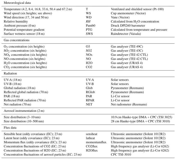
Table 1. Variables, symbols and measurement devices used in this study.
Meteorological data
Temperature (4.2, 8.4, 16.8, 33.6, 50.4 and 67.2 m) T Ventilated and shielded sensor (Pt-100) Wind speed (six heights; see above) WS Cup anemometer (Vector)
Wind direction (17, 34 and 50 m) WD Vane (Vector)
Relative humidity RH Calculated from H2O concentration Ambient pressure (0 m) Pamb0 Druck DPI260 barometer
Potential temperature gradient PTG Calculated from temperature and pressure Surface wetness sensor (18 m) SWS Raindetector (Vaisala)
Gas concentrations
O3concentration (six heights) O3 Gas analyser (TEI 49C) SO2concentration (six heights) SO2 Gas analyser (TEI 43C) NOxconcentration (six heights) NOx Gas analyser (TEI 42 CTL) NO concentration (six heights) NO Gas analyser (TEI 42 CTL) H2O concentration (six heights) H2O Gas analyser (URAS 4) CO2concentration (six heights) CO2 Gas analyser (URAS 4) Radiation
UV-A (18 m) UV-A Solar sensors UV-B (18 m) UV-B Solar sensors
Global radiation (18 m) Glob Pyranometer (Reemann) Reflected global radiation (70 m) RGlob Pyranometer (Reemann)
PAR (18 m) PAR Li-Cor sensor
Reflected PAR radiation (70 m) RPAR Li-Cor sensor
Net radiation (70 m) NET Net radiometer (Reemann) Aerosol instrumentation (2 m)
Size distribution (3–10 nm) 10.9 cm Hauke-type DMA + CPC (TSI 3025) Size distribution (10–500 nm) 28 cm Hauke-type DMA + CPC (TSI 3010) Flux data
Sensible heat (eddy covariance (EC); 23 m) sensheat Ultrasonic anemometer (Solent 1012R2) Latent heat (eddy covariance (EC); 23 m) latheat Ultrasonic anemometer (Solent 1012R2) Momentum flux (eddy covariance (EC); 23 m) momentumflux Ultrasonic anemometer (Solent 1012R2) Concentration fluctuations of CO2 (EC; 23 m) CO2flux High frequency gas analyser (Li-Cor 6262) Concentration fluctuations of H2O (EC; 23 m) H2Oflux High frequency gas analyser (Li-Cor 6262) Concentration fluctuations of aerosol particles (EC; 23 m) CPC TSI-3010
A standard approach in estimating the performance of classification methods is to use cross-validation. The data is repeatedly split into two independent sets, one of which is used as the training set to fit the model in question, and the other is used as the test set to to obtain an unbiased estimate for the classification error.
We evaluate the performance of the methods by computing the misclassification rate:
error=Nmissed+Nfalse Ntotal
·100%,
where Nmissedis the number of event days classified as
non-events, Nfalse is the number of nonevent days classified as
event days, and Ntotal is the total number of days classified.
After cross-validation we report the average misclassification
rate together with 95% confidence intervals. We frequently also list the proportion of missed events and false events: missed = Nmissed
Ntotal
·100%, false =Nfalse Ntotal
·100%. Most classification methods require all classes to have ap-proximately of the same number of cases.
3.3.1 Linear methods for classification
For an important class of classification methods the bound-aries separating the objects to be classified are linear. There are a number of methods to find a linear separating hyper-plane. We briefly describe some of them. For more details see e.g. the reference mentioned earlier.
In Linear Discriminant Analysis (LDA) the goal is to find a set of linear combinations of the original variables so that when the data is projected onto the subspace spanned by these vectors the within-class scatter is minimized and the between-class scatter is maximized. Such linear combina-tions are called linear discriminants. In a two-class case such as ours we only look for one linear discriminant. The first linear discriminant is the normal of the hyperplane separat-ing the two classes. It therefore also tells how event days are separated from nonevent days. LDA is closely related to multivariate analysis of variance (MANOVA).
One can use LDA for fitting quadratic boundaries by adding the second order terms to the data matrix. For ex-ample, in the two variable case we add to the variables x and y the second order terms x2, y2 and xy. We then do LDA in this five-dimensional space with coordinates (x, y, x2, y2, xy) instead of the original two-dimensional one with coordinates (x, y). We shall refer to this method as LDAQ.
Linear regression in turn predicts the output y via a linear model y = β0+ n X j =1 βjxj,
where x=(xj)nj =1is our n−dimensional input data. This is usually used to predict quantitative outputs, but it can be used for classification tasks too. In the classification case we de-fine y to be one for event days and zero for nonevent days, and fit the regression model accordingly. Our input data con-sists of the measurement vectors for each day.
Logistic regression belongs to generalized linear models. Here we want to formulate a model for the probability that the output y is 1 given the input x: p(y=1|x). We could use a linear model for this, but this is not ideal. For example, a linear model can take values outside the interval [0, 1], which are not meaningful. Instead, we modify the model by trans-forming the probability nonlinearly so that it can be modeled by a linear combination. In logistic regression this nonlinear-ity is the logistic function:
log p(y =1|x) 1 − p(y = 1|x),
which is modeled linearly, i.e.
log(p/(1 − p)) = β0+
n X
j =1
βjxj.
Support vector machines (SVM) belong to kernel meth-ods, in which the idea is to map the original data (usually nonlinearly) into a (higher dimensional) feature space and do e.g. classification there (Shawe-Taylor and Christianini, 2004). When using a linear kernel this method falls into the category of linear methods. In this case we lose some of the potential of the method, but we are able to keep track of the
variables. Sacrificing linearity (which in any case is probably too strict an assumption in our case) we have a choice of a wide variety of kernels. Most commonly used ones include polynomial kernels and RBF (radial basis function) kernels. Polynomial kernels of degree two have been tried out in our study, but since the results for a wide variety of parameter choices were constantly worse than for linear kernels, the re-sults for these are omitted. We have used the LS-SVM Tool-box for Matlab (Pelckmans et al., 2003).
3.3.2 Other classification methods
With the SVMs we already moved out of the realm of linear methods. Here we describe two other nonlinear classification methods that have been used.
K-nearest neighbor classification takes a point in the test set, compares it with all the points in the training set, and de-cides the class by looking at the class of the K nearest neigh-bors of the point. In our case, for K=10, the event status of a day in the test set is decided by looking at the event status of the 10 days most closely resembling the day under inspec-tion. This gives us a feel for how close the event days are to each other. However, we do not gain information about in what aspects the event days are similar to eachother.
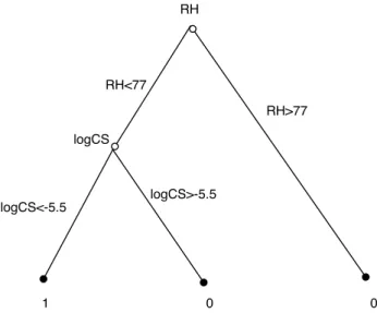
Classification trees (Breiman et al., 1984) partition the fea-ture space into a set of rectangles, and then assign a constant class in each one. We first split the space into two regions, and assign a class to each one. The variable and the split-point are selected to minimize classification error. Then both regions are split into two more regions, and this process is continued until some stopping criterion is applied. This can be visualized as a tree, see Fig. 1. The topmost variable (RH) is the single variable with the best classification performance. On the left branch of the tree we have the condensation sink. This is the best variable (in terms of classification perfor-mance) in distinguishing event days from nonevent ones in the half plane RH<77. Compare this to Fig. 4. The left-most branch of the tree presented in Fig. 1 corresponds to the lower left corner of Fig. 4.
3.3.3 Feature selection
A simple approach to gain insight on the importance of dif-ferent variables in explaining events is to take all pairs of variables and see how well the days are classified as event or nonevent days on the basis of the values of each pair. The same can be done for each triplet of variables, but beyond that the complexity of the problem makes this approach im-practical.
Of course, it is hardly likely to find a satisfactory expla-nation for such a complex phenomenon by just using two or three variables. An alternative is to use a stepwise approach (Hand et al., 2001). In doing stepwise forward selection of variables we start with the variable which gives the best clas-sification result by itself, and on each step add the variable
RH logCS RH>77 RH<77 logCS>-5.5 logCS<-5.5 1 0 0
Fig. 1. A simple decision tree. Take a test day and start from the
top of the tree. If RH is larger than the value indicated, follow the right branch and conclude that the test day is not an event day. In the opposite case follow the left brach and come to the next variable: the condensation sink. If it is larger than the indicated value, again follow the right branch and conclude that the day is not an event day; in the opposite case the day is classified as an event day.
Table 2. Number of different types of days in each cluster.
cluster 4 3 2 1
days 20 218 164 151
event days 1 22 93 140
nonevent days 19 196 71 11
percentage of event days 5 10 57 93
which results in the best classification. In doing stepwise backward selection of variables, we start with all variables, and on each step leave out one variable, chosen so that the classification result is optimized. In forward selection there is the risk that the combined effect of some set of variables is missed. In backwards selection it is possible that we discard a significant variable at an early stage. For our data back-wards selection performed poorly, so the results are omitted. A tempting approach is to look at the weights given by linear regression for each variable, or the normal of the sepa-rating hyperplane in the case of linear discriminant analysis. One could argue that these tell about the relative importance of the variables. This, however, is not true when there are strongly correlating variables so one should only use this proach with extreme caution: for our data set it was not ap-plicable. 0 50 100 150 200 250 300 350 400 1 2 3 4
Day of the year
Cluster number
Fig. 2. The seasonal distribution of days in each cluster. Each color
represents a different cluster. The topmost row shows the days in the cluster, below that extra marks denote the event days.
4 Results
4.1 Clustering
We used K-means clustering to cluster the days into four clusters. The results are very good: the algorithm does not use event information for clustering, yet it produces clusters with very few event days, as well as one with over 90% event days.
The temporal distribution of these days is presented in Fig. 2. Note the temporal cohesion of the clusters, even though the calendar time is not used in the clustering. Clus-ter 1 consists almost solely of event days, whereas clusClus-ters 3 and 4 have almost no events. From top to bottom, the counts for days and event days for each cluster are presented in Ta-ble 2.
We observe four robust clusters: spring&fall days ter 1), summer days (cluster 2), low radiation days (clus-ter 3) and polluted days (clus(clus-ter 4). The names describing clusters 3 and 4 are derived by looking at the cluster centers of these clusters. The cluster centers, describing the typi-cal values of each variable in each cluster, are presented in Fig. 3. One can see that the best parameters to separate the event clusters (1 and 2) from non-event clusters (3 and 4) are relative humidity, global radiation and sensible heat. Also the mean of ozone and carbon dioxide concentrations have a separation power. Most of the event days fall in to clusters 1 and 2. The main difference between these clusters is the time of the year and the related physical parameters. The summer days in cluster 2 have higher temperatures along with an el-evated concentration of water and higher daily variability of CO2, O3 and H2O concentrations. Also the CO2 and H2O
−3 −2 −1 0 1 2 3 4 5
Pamb0 mean T hi mean WS hi mean NO hi mean NOx hi mean O3 hi mean SO2 hi mean H2O hi mean CO2 hi mean RH hi mean PTG mean Glob mean SWS mean SinWD mean CosWD mean logCS mean sensheat mean H2Oflux mean momflux mean CO2flux mean
Cluster 1 Cluster 2 Cluster 3 Cluster 4 −3 −2 −1 0 1 2 3 4
Pamb0 std T hi std WS hi std NO hi std NOx hi std O3 hi std SO2 hi std H2O hi std CO2 hi std RH hi std PTG std Glob std SWS std SinWD std CosWD std logCS std sensheat std H2Oflux std momflux std CO2flux std
Cluster 1 Cluster 2 Cluster 3 Cluster 4
Fig. 3. The center of each cluster can be thought of as a prototype
representative of the cluster. Here are the cluster centers. The data is normalized, so the values of each variable for each cluster only indicate whether the variable is above or below average. The colors are as in Fig. 2: from least to most eventful clusters blue, cyan, magneta, red.
fluxes differ in clusters 1 and 2. The condensation sink has low values in the cluster with most of the events.
4.2 Results using classification methods
The main result given by the wide range of classification methods used is that the most important variables in explain-ing the nucleation events are the means of the relative humid-ity (RH) and the logarithm of the condensation sink. This is supported by a number of different approaches.
– When fitting a decision tree to the data, these are the
top two variables selected in most cases. Moreover, on the test set the tree involving only these variables (see
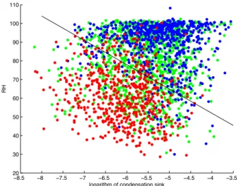
−8.5 −8 −7.5 −7 −6.5 −6 −5.5 −5 −4.5 −4 −3.5 20 30 40 50 60 70 80 90 100 110
logarithm of condensation sink
RH
Fig. 4. Best predicting pair of variables, when means are computed
for each day in the time window from sunrise to sunset. Nonevents are blue, events are red and undefined days are green. Note, that the distribution of undefined days is similar to that of the days defined as either event or nonevent days. Also shown is the optimal separating line as given by LDA.
Fig. 1) performs frequently as well as more complicated trees, which tend to overfit.
– These are also the two first variables selected when
do-ing forward stepwise selection of variables usdo-ing any of the linear methods.
– These two variables form the best pair of variables.
They also are almost always included among the best three variables. The best pairs were sought after using both linear regression and linear discriminant analysis. For the best triplets, only linear regression was used. The performance of a number of methods using only RH and the logarithm of the condensation sink is summarized in Table 3. Each method was run 1000 times using different training and test sets, and the average percentage of errors and 95% confidence intervals for the errors were computed.
In Table 4 we have summarized the performance of a few of the top ranking pairs using LDA. We see that RH and the condensation sink have the best performance. The other methods yield similar results.
This can be compared to the performance of a few of the top ranking triplets using linear regression, summarized in Table 5. It is evident that there is no “best triplet” as the 95% confidence intervals of all of these overlap. In fact, for 127 triplets the 95% confidence intervals overlap with that of the best ranked one, topmost in this table, and 80 of these have confidence intervals which overlap that of the best pair; not one triplet is clearly better than the best pair.
Table 3. Average error rates over 1000 runs and 95% confidence intervals for different classification methods using means of RH low and
the logarithm of the condensation sink. 10-NN refers to the 10 nearest neighbor method.
Method error rate (%) false events (%) missed events (%) LDA 11.9±0.2 11.7±0.2 12.2±0.3 logistic regression 12.3±0.2 11.3±0.2 13.3±0.3 linear regression 12.2±0.2 14.8±0.2 9.2±0.2 SVM (linear kernel) 11.9±0.2 11.7±0.2 12.0±0.2 10-NN 13.8±0.2 14.6±0.3 12.8±0.3 LDAQ 12.7±0.2 10.6±0.3 15.0±0.3 decision trees 14.2±0.2 6.5±0.2 23.1±0.4
Table 4. Average error rates over 40 runs for top ranking pairs of
variables using LDA.
Variables error (%)
RH low mean, logCS mean 11.7±0.7
RH high mean, logCS mean 12.1±0.7 H2O low mean, RH high mean 13.4±0.9 H2O high mean, RH high mean 13.5±0.9 H2O high mean, RH low mean 13.8±0.9 RGlob std, logCS mean 13.8±0.7 H2O low mean, RH low mean 13.9±0.9 RGlob mean, logCS mean 13.9±0.8 Glob mean, logCS mean 14.0±0.9 sensheat mean, logCS mean 14.3±0.8
We have demonstrated above that relative humidity and the condensation sink are the most significant variables ex-plaining the nucleation events. All of the linear classification methods had an error rate of approximately 12% when using only these two variables. It seems reasonable to expect, that adding variables to the model would improve classification results. But here we run into the problem demonstrated by the best triplets: there are too many choices of variables with equal performance.
When using stepwise addition of variables together with any of the classification methods, different runs (using dif-ferent training sets) yield difdif-ferent sets of variables with ap-proximately equal performance. The same is true for deci-sion trees. It is not true that the two variable model could not be improved by adding variables, but the set of variables that can be added for improved performance is not unique. This is in fact quite a typical situation in data mining ap-plications whenever there are correlations between variables. Table 6 presents the results for two sets of forward addition of variables using LDA. After RH and the logarithm of the condensation sink are added the lists diverge. Yet the perfor-mance of the methods after 10 variables are chosen are not significantly different.
Table 5. Average error rates over 20 runs for some top ranking
triplets of variables using linear regression.
Variables error(%)
RH low mean, logCS mean, SO2 high std 11.6±1.3
RH low mean, logCS std, H2O low mean 11.6±1.5
RH low mean, logCS mean, SWS std 11.7±1.4 H2O high mean, logCS std, Glob mean 11.8±1.2
RH low mean, logCS mean, O3 low mean 11.9±1.5
RH high mean, logCS mean, NO low std 11.9±1.5
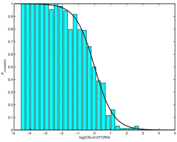
Finally, let us return to the two variables, RH and the con-densation sink. We can project the data onto the first linear discriminant. The first linear discriminant is the normal of the line separating events from nonevents in Fig. 4, so it is the direction giving optimal separation for events and nonevents. Points in one end of the linear discriminant are mainly event days, and points in the other end are mainly nonevent days. From this projected data we can compute the probability of having an event day at each point. This is done by first com-puting the proportion of events in each interval of a fixed width, and then fitting a logistic model to this data. This is illustrated in Fig. 5. We get the following nucleation param-eter describing the probability of nucleation:
Pnucl= 1 1 + exp(β1log(CS) + β2(RH )) , (1) β1=1.7 β2=0.13. 5 Discussion 5.1 Condensation sink
Low condensation sink values favour nucleation due to two basic reasons (Kulmala et al., 2005):
– The existing aerosol population depletes the ambient air
Table 6. Two sets of forward addition of variables using LDA. The variables are listed in the order they are added to the model. Each addition is done based on average error rate over 100 runs on different training and test sets, given in the second column. The 95% confidence intervals are be about ±0.6. After the first two variables the lists diverge.
Set 1 Set 2
variable error variable error
RH high mean 17.8 RH high mean 17.5 logCS mean 12.1 logCS mean 12.4 T high std 12.3 SO2high std 12.0 logCS std 11.8 momflux std 11.1 CO2high mean 11.1 O3high std 11.0 O3high std 10.8 SWS std 10.7
RH high std 10.6 O3high mean 10.7 WS high mean 10.5 SO2high mean 10.8 SO2high std 10.2 SWS mean 10.5 SinWD mean 9.9 CosWD std 10.7
sink is high, no vapour is available to grow the parti-cles to larger sizes, and they are lost by coagulation and deposition. It is also possible that these vapours partici-pate in the nucleation process itself.
– A higher condensation sink signifies also a higher
coag-ulation rate of newborn particles, meaning a shorter life-time of these particles. The loss rate due to coagulation is higher the smaller the particle is. Thus, a lower sink increases the likelihood of a nucleated particle growing large enough to survive.
These two processes work the same direction. 5.2 Relative humidity
Besides the impact of relative humidity on the condensation sink by forcing the present particles to grow by the uptake of water molecules and thus increasing the available surface area for condensable vapours, RH affects the solar radiation reaching the atmospheric boundary layer. The effect of RH on solar radiation is due to its linkage to clouds, fog and rain, since there is a strong correlation between RH and cloudi-ness. Thus, at least part of the reducing effect of relative humidity might be caused by the reduction of solar radiation. Linked to this is the effect of relative humidity on the gas-phase chemistry of compounds involved in the nucleation and the subsequent growth. Note that these reaction mecha-nisms can occur only during cloud free days, since the solar radiation is one of the key elements in the reaction chain.
When assuming that the nucleation process is started by the formation of clusters of either binary or ternary sulphuric acid (H2SO4) reactions (Kulmala et al., 2004b), including
−5 −4 −3 −2 −1 0 1 2 3 4 5 0 0.1 0.2 0.3 0.4 0.5 0.6 0.7 0.8 0.9 1 log(CS)+0.077(RH) Pnucleation
Fig. 5. The proportion of events (light blue bars) along the first linear discriminant (x-axis) and the logistic model Eq. (1) fitted to this.
either water vapour or water vapour and ammonia, the for-mation of sulphuric acid is directly linked to the forfor-mation of OH. This depends on the amount of solar radiation and the amount of water vapour present, both of which increase the OH concentration. However, the higher the water vapour concentration the lower the solar radiation reaching the atmo-spheric boundary layer. Consequently there is a maximum production level between low and high relative humidity: in-creasing relative humidity will first result in an increase of sulphuric acid formation, but this will decline after the ap-pearance of clouds.
A second possibility is that secondary organics, formed by gas-phase reactions of emitted reactive hydrocarbons, cause the initiation of nucleation. These compounds can contribute via two different processes: by condensation on the clusters and thus activating them by growing to detectable sizes (ra-dius of 3 nm) (Kerminen et al., 2004) or by forming new par-ticles by themselves (Bonn and Moortgat, 2003). The most important ones are the reactive mono- and sesquiterpenes re-leased by the biosphere. Smog chamber studies indicate that the reaction with ozone form the products of lowest volatil-ity, among the three possible oxidation reactions, compet-ing at ambient conditions. Bonn et al. (2002) and Bonn and Moortgat (2002, 2003) have found that only the ozonolysis is affected by the presence of water vapour in nucleation and subsequent growth. This is caused by the reaction of water vapour with the so-called stabilized Criegee biradical (SCI), formed during the first reaction steps of the terpene. The former suppresses the formation of the nucleating agent by competition.
Since the impact of both relative humidity and the con-densational sink are linked to each other, and furthermore
to chemical compounds, there is currently no way to sepa-rate the contribution of possible nucleation mechanisms and causes based on our study.
5.3 Other parameters
Previous work has indicated that nucleation events are largely explained by three parameters: temperature, water content and radiation (Boy and Kulmala, 2002). This study supports these findings with the exception of radiation. This might be due to the strong seasonal variation of the solar ra-diation. In our study we found two clearly important param-eters, relative humidity and the condensation sink. Radiation has an effect, but it is no more important than O3, SO2 or
NO. These variables appear among the best variables after relative humidity and condensation sink in different statisti-cal methods and in repeated runs, but there is no clear way to choose one over the others. One reason could be the in-ternal correlations between the variables: selecting one of them explains the latent variable behind all of them. Alterna-tively, the variables are related to less important nucleation processes.
The variables we found to be important are related to the mechanisms that prevent nucleation from starting and parti-cles from growing to detectable sizes. This finding supports the hypothesis presented by Kulmala et al. (2000) that there exists a reservoir of thermodynamically stable clusters (TSC) in the atmosphere, which act as initial nuclei for particle for-mation. However, TSC grow to detectable sizes only under certain conditions. The mechanisms for the growth of TSC are either self-coagulation of TSC, condensation of vapours, or both. High relative humidity and a high condensation sink decrease concentrations of condensable gases in the atmo-sphere and thus prevent nucleation from starting and parti-cles from growing. Similarly the high amount of preexisting particles act as a coagulation sink for the TSC and for freshly formed, below 3 nm particles. By coagulating onto preexist-ing particles the probability for self-coagulation of TSC will decrease and the nucleation process will stop. Still, from the result of this study it cannot be concluded whether the TSC really act as initial nuclei for nucleation or whether some new clusters are formed.
6 Conclusions
In this study we found that aerosol particle formation events observed in boreal forests are connected with two variables, the condensation sink and relative humidity. The unfavor-able effect of the condensation sink is supposed to be due to uptake of freshly-nucleated clusters and condensing vapours. The variables found to be important in this study are re-lated to the mechanisms that prevent nucleation from starting and particles from growing to detectable sizes. The outcome supports the idea of having processes that cause nucleation
and processes that prevent nucleation. The preventing mech-anisms are the more important ones, and nucleation only oc-curs when the preventing mechanisms fail.
One possible explanation for the adverse connection of high relative humidity is due to its effect on terpene oxida-tion products. In the presence of water vapour the stabilized Criegee biradical (SCI) produce high volatility compounds, whereas with low RH chemical reactions lead to low volatil-ity compounds. Such low-volatilvolatil-ity compounds can con-densate onto nucleated clusters or nucleate by themselves. Also the effect of NOxand O3support this chemical reaction
route. In addition to its effect on chemical reactions, high relative humidities increase the condensation sink due to the hygroscopic growth of aerosol particles. High relative hu-midity can also affect particle formation due to its linkage to clouds, fog and rain since reduced solar radiation may inhibit photochemical reactions related to nucleating vapours in the atmosphere.
Although we found a connection between the occurrence of nucleation and two key variables, the detailed chemistry still remains speculative. One missing link in our study is the concentration of biogenic Volatile Organic Compounds (VOC) emissions, which are expected to be of high impor-tance even at the low concentrations. Unfortunately, we were not able to measure VOCs since especially the more reactive compounds are extremely hard to measure with the current instrumentation.
One possible cause of confusion is the possibility of two or even more different nucleation mechanisms acting simultaneously in the atmosphere. One such combination is clear-air nucleation vs. pollution nucleation, another pos-sibility is combination of neutral and ion-induced nucleation.
Edited by: A. Laaksonen
References
Aalto, P., H¨ameri, K., Becker, E., Weber, R., Salm, J., M¨akel¨a, J. M., Hoell, C., O’Dowd, C. D., Karlsson, H., Hansson, H.-C., V¨akev¨a, M., Koponen, I. K., Buzorius, G., and Kulmala, M.: Physical characterization of aerosol particles during nucleation events, Tellus, 53B, 344–358, 2001.
Aubinet, M., Grelle, A., Rannik, A. I. U., Moncrieff, J., Foken, T., Kowalski, A. S., Martin, P. H., Berbigier, P., Clement, C. B. R., Elbers, I., Granier, A., Gr¨unwald, T., Pilegaard, K. M. K., Reb-mann, C., Snijders, W., Valentini, R., and Vesala, T.: Estimates of the annual net carbon and water exchange of forests: The EU-ROFLUX methodology, Advances in Ecological Research, 30, 113–175, 2001.
Birmili, W. and Wiedensohler, A.: New particle formation in the continental boundary layer: Meteorological and gas phase pa-rameter influence, Geophys. Res. Lett., 27, 3325–3328, 2000. Bonn, B. and Moortgat, G.: Sesquiterpene ozonolysis: Origin of
atmospheric new particle formation from biogenic hydrocarbons, Geophys. Res. Lett., 30, 1585–1588, 2003.
Bonn, B. and Moortgat, G. K.: New particle formation during α-and β-pinene oxidation by O3, OH and NO3, and the influence
of water vapour: Particle size distribution studies, Atmos. Chem. Phys., 2, 183–196, 2002,
SRef-ID: 1680-7324/acp/2002-2-183.
Bonn, B., Schuster, G., and Moortgat, G. K.: Influence of water va-por on the process of new particle formation during monoterpene ozonolysis, J. Phys. Chem. A, 106, 2869–2881, 2002.
Boy, M. and Kulmala, K.: Nucleation events in the continental boundary layer: Influence of physical and meteorological param-eters, Atmos. Chem. Phys., 2, 1–16, 2002,
SRef-ID: 1680-7324/acp/2002-2-1.
Breiman, L., Friedman, J. H., Olshen, R. A., and Stone., C. J.: Clas-sification and Regression Trees, Wadsworth, 1984.
Dal Maso, M., Kulmala, M., Riipinen, I., Wagner, R., Hussein, T., Aalto, P. P., and Lehtinen, K. E. J.: Formation and Growth of Fresh Atmospheric Aerosols: Eight Years of Aerosol Size Dis-tribution Data from SMEAR II, Hyytiala, Finland, Boreal Env. Res., 10, 323–336, 2005.
Davies, D. and Bouldin, D. W.: A Cluster Separation Measure, IEEE Transactions on Pattern Analysis and Machine Learning, 1, 224–227, 1979.
Dunn, M. E., Pokon, E. K., and Shields, G. C.: Thermodynamics of Forming Water Clusters at Various Temperatures and Pressures by Gaussian-2, Gaussian-3, Complete Basis Set-QB3, and Com-plete Basis Set-APNO Model Chemistries; Implications for At-mospheric Chemistry, J. Am. Chem. Soc., doi:10.1021/ja03892, 2004.
Eichkorn, S., Wilhelm, S., Aufmhoff, H., Wohlfrom, K., and Arnold, F.: Cosmic ray-induced aerosol formation: First evi-dence from aircraft-based ion mass spectrometer measurements, Geophys. Res. Lett., 29, 14, 2002.
Falge, E., Baldocchi, D., and Olson, R.: Gap filling strategies for defensible annual sums of net ecosystem exchange, Agric. For. Meteorol., 107, 43–69, 2001.
Fuchs, N. A. and Sutugin, A. G.: Highly dispersed aerosols., Ann Arbour Science Publishers, Ann Arbour, London, 1970. Hand, D., Mannila, H., and Smyth, P.: Principles of Data Mining,
MIT Press, 2001.
Hastie, T., Tibshirani, R., and Friedman, J.: The Elements of Statis-tical Learning, Springer, 2001.
Hotelling, H.: Analysis of a Complex of Statistical Variables into Principal Components, J. Educational Psychology, 24, 417–441, 498—520, 1933.
IPCC: Climate Change 2001: The Scientific Basis, Contribution of Working Group 1 to the Third Assessment Report of the In-tergovermental Panel on Climate Change, Cambridge University Press, Cambridge, UK, 2001.
Keeling, C. D., Bacastow, R. B., and Whorf, T. P.: Measurements of the concentration of carbon dioxide at Mauna Loa Observatory, Hawaii, Oxford University Press, New York, 1982.
Kerminen, V. M., Anttila, T., Lehtinen, K. E. J., and Kulmala, M.: Parameterization for atmospheric new-particle formation: Appli-cation to a system involving sulfuric acid and condensable water-soluble organics., Aer. Sci. Technol., 38, 1001–1008, 2004. Koponen, I., Virkkula, A., Hillamo, R., Kerminen, V. M., and
Kul-mala, M.: Number size distributions and concentrations of ma-rine aerosols: Observations during a cruise between the English Channel and the coast of Antarctica, J. Geophys. Res., 107, 4753, doi:10.1029/2002JD002533, 2002.
Korhonen, P., Kulmala, M., Laaksonen, A., Viisanen, Y., McGraw,
R., and Seinfeld, J.: Ternary nucleation of H2SO4, NH3and H2O in the atmosphere, J. Geophys. Res., 104, 26 349–26 353, 1999. Kulmala, M., Pirjola, L., and M¨akel¨a, J. M.: Stable sulphate clusters
as a source of new atmospheric particles, Nature, 404, 66–69, 2000.
Kulmala, M., Kerminen, V.-M., Anttila, T., Laaksonen, A., and O’Dowd, C.: Organic aerosol formation via sulphate cluster activation, J. Geophys. Res., 109, doi:10.1029/2003JD003961, 2004a.
Kulmala, M., Vehkam¨aki, H., Pet¨aj¨a, T., Dal Maso, M., Lauri, A., Kerminen, V.-M., Birmili, W., and McMurry, P.: Formation and growth rates of ultrafine atmospheric particles: a review of ob-servations, J. Aerosol Sci., 35, 143–176, 2004b.
Kulmala, M., Pet¨aj¨a, T., M¨onkk¨onen, P., Koponen, I. K., Dal Maso, M., Aalto, P. P., Lehtinen, K. E. J., and Kerminen, V.-M.: On the growth of nucleation mode particles: source rates of condensable vapor in polluted and clean environments, Atmos. Chem. Phys., 5, 409–416, 2005,
SRef-ID: 1680-7324/acp/2005-5-409.
Laakso, L., Pet¨aj¨a, T., Lehtinen, K., Kulmala, M., Paatero, J., H˜orrak, U., Tammet, H., and Joutsensaari, J.: Ion production rate in a boreal forest based on ion, particle and radiation mea-surements, Atmos. Chem. Phys., 4, 1933–1943, 2004,
SRef-ID: 1680-7324/acp/2004-4-1933.
MacQueen, J.: Some methods for classification and analysis of mul-tivariate observations, in Proceedings of the Fifth Berkeley Sym-posium on Mathematical Statistics and Probability, edited by: Le Cam, L. M. and Neyman, J., vol. I, University of California Press, 281–297, 1967.
M¨akel¨a, J. M., Aalto, P., Jokinen, V., Pohja, T., Nissinen, A., Palm-roth, S., Markkanen, T., Seitsonen, K., Lihavainen, H., and Kul-mala, M.: Observations of ultrafine aerosol particle formation and growth in boreal forest, Geophys. Res. Lett., 24, 1219–1222, 1997.
Moler, C. B.: Numerical computing with MATLAB, Society for In-dustrial and Applied Mathematics, Philadelphia, PA, USA, 2004. M¨onkk¨onen, P., Koponen, I., Lehtinen, K., H¨ameri, K., Uma, R., and Kulmala, M.: Measurements in a highly polluted Asian mega city: Observations of aerosol number size distributions, modal parameters and nucleation events, Atmos. Chem. Phys., 5, 57– 66, 2005,
SRef-ID: 1680-7324/acp/2005-5-57.
Nilsson, E. D., Paatero, J., and Boy, M.: Effects of air masses and synoptic weather on aerosol formation in the continental bound-ary layer, Tellus, 53B, 2001.
O’Dowd, C. D., Aalto, P., H¨ameri, K., Kulmala, M., and Hoffmann, T.: Atmospheric particles from organic vapours, Nature, 416, 497–498, 2002a.
O’Dowd, C. D., Jimenez, J. L., Bahreini, R., Flagan, R. C., Seinfeld, J. H., H¨ameri, K., Pirjola, L., Kulmala, M., Jennings, S. G., and Hoffmann, T.: Marine aerosol formation from biogenic iodine emissions, Nature, 417, 632–636, 2002b.
Pelckmans, K., Suykens, J., Van Gestel, T., De Brabanter, J., Lukas, L., Hamers, B., De Moor, B., and Vandewalle, J.: LS-SVMlab Toolbox User’s Guide, Tech. Rep. ESAT-SCD-SISTA 02-145, Katholieke Universiteit Leuven, 2003.
Pirjola, L. and Kulmala, M.: Modelling the formation of H2SO4-H2O particles in rural, urban and marine conditions, Atmos. Res., 46, 1998.
Rannik, U.: On the surface layer similarity at a complex forest site, J. Geophys. Res., 103, 8685–8697, 1998.
Ruuskanen, T., Reissell, A., Keronen, P., Aalto, P., Laakso, L., Gr¨onholm, T., Hari, P., and Kulmala, M.: Atmospheric trace gas and aerosol particle concentration measurements in Eastern Lapland, Finland 1992-2001, Boreal Environ. Res., 8, 335-349, 2003.
Shawe-Taylor, J. and Christianini, N.: Kernel methods for pattern analysis, Cambridge University Press, 2004.
Sioutas, C., Pandis, S. N., Allen, D. T., and Solomon, P. A.: Special issue of Atmospheric Environment on findings from the EPA par-ticulate matter supersites program, Atmos. Environ., 38, 3101– 3106, 2004.
Suni, T., Rinne, J., Reissell, A., Altimir, N., Keronen, P., Rannik, U., Dal Maso, M., Kulmala, M., and Vesala, T.: Long-term mea-surements of surface fluxes above a Scots pine forest in Hyyti¨al¨a, Southern Finland, 1996–2001, Boreal Environ. Res., vol. 8, 287– 301, 2003.
Twomey, S.: Pollution and planetary albedo, Atmos. Environ., 8, 1251–1256, 1974.
Vesala, T., Haataja, J., Aalto, P., Altimir, N., Buzorius, G., et al.: Long-term field measurements of atmosphere-surface interac-tions in boreal forest ecology, micrometeorology, aerosol physics and atmospheric chemistry, Trends in Heat, Mass and Momen-tum Transfer, 4, 17–35, 1998.
Weber, R. J., McMurry, P. H., Eisele, F. L., and Tanner, D. J.: Mea-surements of expected nucleation precursor species and 3-500-nm diameter particles at Mauna Loa observatory, Hawaii, J. At-mos. Sci., 52, 2242–2257, 1995.