Information on the early Holocene climate constrains the summer sea ice projections for the 21st century

HAL Id: hal-00298097

https://hal.archives-ouvertes.fr/hal-00298097

Submitted on 20 Dec 2007

HAL is a multi-disciplinary open access

archive for the deposit and dissemination of

sci-entific research documents, whether they are

pub-lished or not. The documents may come from

teaching and research institutions in France or

abroad, or from public or private research centers.

L’archive ouverte pluridisciplinaire HAL, est

destinée au dépôt et à la diffusion de documents

scientifiques de niveau recherche, publiés ou non,

émanant des établissements d’enseignement et de

recherche français ou étrangers, des laboratoires

publics ou privés.

the summer sea ice projections for the 21st century

H. Goosse, E. Driesschaert, T. Fichefet, M.-F. Loutre

To cite this version:

H. Goosse, E. Driesschaert, T. Fichefet, M.-F. Loutre. Information on the early Holocene climate

con-strains the summer sea ice projections for the 21st century. Climate of the Past, European Geosciences

Union (EGU), 2007, 3 (4), pp.683-692. �hal-00298097�

Clim. Past, 3, 683–692, 2007 www.clim-past.net/3/683/2007/

© Author(s) 2007. This work is licensed under a Creative Commons License.

Climate

of the Past

Information on the early Holocene climate constrains the summer

sea ice projections for the 21st century

H. Goosse, E. Driesschaert, T. Fichefet, and M.-F. Loutre

Universit´e Catholique de Louvain, Institut d’Astronomie et de G´eophysique G. Lemaˆıtre, Chemin du Cyclotron, 2, 1348 Louvain-la-Neuve, Belgium

Received: 15 August 2007 – Published in Clim. Past Discuss.: 24 August 2007

Revised: 14 November 2007 – Accepted: 2 December 2007 – Published: 20 December 2007

Abstract. The summer sea ice extent strongly decreased in

the Arctic over the last decades. This decline is very likely to continue in the future but uncertainty of projections is very large. An ensemble of experiments with the climate model LOVECLIM using 5 different parameter sets has been performed to show that summer sea ice changes during the early Holocene (8 kyr BP) and the 21st century are strongly linked, allowing for the reduction of this uncertainty. Us-ing the limited number of records presently available for the early Holocene, simulations presenting very large changes over the 21st century could reasonably be rejected. On the other hand, simulations displaying low to moderate changes during the second half of the 20th century (and also over the 21st century) are not consistent with recent observations. Us-ing this very complementary information based on observa-tions during both the early Holocene and the last decades, the most realistic projection with LOVECLIM indicates a nearly disappearance of the sea ice in summer at the end of the 21st century for a moderate increase in atmospheric greenhouse gas concentrations. Our results thus strongly indicate that ad-ditional proxy records of the early Holocene sea ice changes, in particular in the central Arctic Basin, would help to im-prove our projections of summer sea ice evolution and that the simulation at 8 kyr BP should be considered as a standard test for models aiming at simulating those future summer sea ice changes in the Arctic.

1 Introduction

Over the last 30 years, corresponding to the period of satel-lite microwave observations, the annual mean Arctic sea ice extent has decreased at a mean rate of about 0.3×106km2 per decade (Lemke et al., 2007). The summer decline was

Correspondence to: H. Goosse

(hgs@astr.ucl.ac.be)

found to be even larger, with a reduction of 0.6×106km2per decade (Lemke et al., 2007; Stroeve et al., 2007). Those re-cent observed changes have led to considerable attention on the model projections of summer sea ice changes, the even-tuality of a seasonally ice-free Arctic before the end of this century being one of the strongest image associated with fu-ture climate warming (e.g. Arzel et al., 2006; Holland et al., 2006; Zhang and Walsh, 2006; Meehl et al., 2007; Serreze et al., 2007; Schiermeier, 2007).

All the simulations performed in the framework of the In-tergovernemental Panel for Climate Change Fourth Assess-ment Report (IPCC AR4) show that the Arctic sea ice decline will continue during the whole 21st century in response to the increase in the concentrations of atmospheric greenhouse gases (Arzel et al., 2006; Zhang and Walsh, 2006; Meehl et al., 2007; Serreze et al., 2007). However, there is more than a factor three in the estimates of the future trend between the different models, even using an identical scenario for the future evolution of the concentrations of atmospheric green-house gases (Arzel et al., 2006; Zhang and Walsh, 2006; Meehl et al., 2007; Serreze et al., 2007). Reducing the pro-jections uncertainties is thus a major objective of the climate modelling community and a major challenge.

It is customary to assess the quality of models by compar-ing their output with recent observations. In particular, the models not able to reproduce sufficiently well the observed mean Arctic ice extent at the end of the 20th century were discarded in a number of recent analyses (e.g., Arzel et al., 2006; Stroeve et al., 2007). However, the decision to reject a model is partly arbitrary and not consistent across papers (Arzel et al., 2006; Stroeve et al., 2007). Furthermore, the relevance of rejection criteria may also be called into ques-tion because it has been hard to find strong relaques-tionships be-tween the model characteristics simulated at the end of the 20th century and the decrease in sea ice extent obtained dur-ing the 21st century (Arzel et al., 2006; Holland and Bitz, 2003; Flato, 2004). The observed decrease in Arctic sea ice

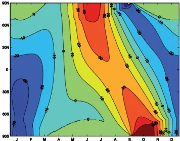
Fig. 1. Deviations from present-day values of the calendar 24 h

mean solar irradiance (daily insolation) at 8 kyr BP (unit is Wm−2).

extent over the last decades provides another test case for models (Arzel et al., 2006; Zhang and Walsh, 2006; Meehl et al., 2007, Serreze et al., 2007; Stroeve et al., 2007). In particular, it is shown in a recent study (Stroeve et al., 2007) that no simulation performed in the framework of the IPCC AR4 is able to reproduce the observed decline in summer ice extent over the last 53 years. This provides evidence that the models underestimate the response of the sea ice to rising concentration of greenhouse gases in the atmosphere. How-ever, there is still the possibility that the recent decline is a very rare event of natural variability that is not captured by the relatively small ensemble of simulations presently avail-able (Stroeve et al., 2007).

Additional constraints on the model behaviour could be provided by simulations devoted to the more distant past such as the mid-Holocene (6 kyr BP, i.e. 6000 years before present) or the last glacial maximum (21 kyr BP) (e.g., Cruci-fix, 2006; Masson-Delmotte et al., 2006). However, only the past periods for which the external forcing is well known, a reasonably large amount of data is available and the variable of interest displays large changes compared to the recent past are expected to provide a stringent test of the model.

The early Holocene is potentially a good candidate to con-strain the analysis of the response of the Arctic summer ice cover to a radiative perturbation. Indeed, the insolation in June at 8 kyr BP was much larger than in recent decades (Berger, 1978), the differences reaching +40 W/m2 in June northward of 65◦N (Fig. 1). Seemingly consistent with this forcing, the various geological reconstructions and model simulations for this period tend to display higher summer temperatures and a lower sea ice extent at high latitudes (e.g., Koc¸ et al., 1993; Duplessy et al., 2001; Vavrus and Harrison, 2003; Braconnot et al., 2007). Here we show how model simulations over this period could help us in reducing the

uncertainties in the projections of the decline of the summer Arctic ice extent during the 21st century. Specifically, we have selected the period around 8 kyr BP because the sea ice changes are larger than for the most classical mid-Holocene period (e.g., Renssen et al., 2005). In this framework, we performed simulations with the three-dimensional climate model LOVECLIM (Driesschaert et al., 2007) using five dif-ferent sets of parameters (called E1 to E5, Appendix A), cho-sen to explore the uncertainty range in these parameters as in Murphy et al. (2004), Stainforth et al. (2005), and Ridley et al. (2007) for instance. Our simulations cover the period from the early Holocene to 2100 AD. For the period 1850– 2100 AD, an ensemble of simulations with slightly different initial conditions is performed to estimate the model internal variability for each parameter set (see Sect. 2). As a con-sequence, we provide here controlled experiments with the same model version spanning the whole time period selected and using the same forcing for all the three-dimensional model parameter sets chosen.

2 Model description and experimental design

LOVECLIM is a three-dimensional Earth system model of intermediate complexity that includes representations of the atmosphere, the ocean and sea ice, the land surface (in-cluding vegetation), the ice sheets and the carbon cycle. In the present study, the ice sheet and carbon cycle com-ponents are not activated and will thus not be described here. The atmospheric component is ECBILT2 (Opseegh et al., 1998), a T21, 3-level quasi-geostrophic model. The oceanic component is CLIO3 (Goosse and Fichefet, 1999), which is made up of an ocean general circulation model coupled to a comprehensive thermodynamic-dynamic sea ice model. Its horizontal resolution is 3◦ by 3◦, and there are 20 levels in the ocean. ECBILT-CLIO is coupled to VECODE, a vegetation model that simulates the dynam-ics of two main terrestrial plant functional types, trees and grasses, as well as desert (Brovkin et al., 2002). Its reso-lution is the same as the one of ECBILT. More information about the model and a complete list of references is avail-able at the following address:http://www.astr.ucl.ac.be/index. php?page=LOVECLIM%40Description.

The model version used here is LOVECLIM1.1. Three main improvements have been incorporated in this version compared to LOVECLIM1.0 (Driesschaert et al., 2007). First, the land surface scheme has been modified (see http:// www.astr.ucl.ac.be/ASTER/doc/E AR SDCS01A v2.pdf) in order to take into account the impact of the changes in veg-etation on the evaporation (transpiration) and on the bucket depth (i.e. the maximum water that can be hold in the soil). Second, the emissivity, which was the same for all the sur-face types in LOVECLIM1.0, is now different for land, ocean and sea ice. Third, in order to reduce the artificial vertical diffusion in the ocean caused by numerical noise, the

Corio-H. Goosse et al.: Summer sea ice during the early Holocene 685 lis term is now treated in a fully implicit way in the equation

of motion for the ocean, while a semi-implicit scheme was used in LOVECLIM1.0 (see also Appendix A).

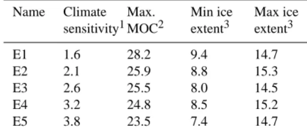
In order to obtain the five model parameter sets considered here, different parameter values have been selected, each of them being in the range of uncertainty of the parameter con-sidered (Appendix A). The goal is, on the one hand, to pro-duce reasonable simulations of the present-day climate (Ta-ble 1), which have similar qualities when compared to the ob-servations in all the regions of the world and for a wide range of variables (surface temperature, precipitation, oceanic and atmospheric circulations, sea ice concentration, radiative ex-changes at the top of the atmosphere). On the other hand, these model parameter sets must lead to clearly contrasted model responses to a perturbation. In particular, the cli-mate sensitivities cover a range from 1.6 to 3.8 K (Table 1). The climate sensitivity is defined here as the global surface temperature change after 1000 y in an experiment performed with LOVECLIM in which the CO2concentration increases from pre-industrial level by 1% per year and is maintained constant after 70 y of integration when it reaches a value equal to two times the pre-industrial level. Such a simula-tion is a classical benchmark to compare different model re-sponses to a radiative perturbation.

Three types of simulations, launched for the five param-eter sets, are conducted with the model. First, a quasi-equilibrium simulation with a constant forcing correspond-ing to pre-industrial conditions is performed with the CO2, CH4 and N2O concentrations in the atmosphere set to 277.6 ppmv, 628.2 ppbv, 267.4 ppbv, respectively. Second, a quasi-equilibrium simulation is carried out with orbital pa-rameters and greenhouse gas concentrations corresponding to the 8 kyr BP conditions. In this experiment, the CO2, CH4 and N2O concentrations are maintained constant at values of 260.6 ppmv, 701.5 ppbv, 267.4 ppbv, respectively. Third, a transient simulation is run from 8 kyr BP to year 2100 AD, starting from the quasi-equilibrium obtained for 8 kyr BP. Be-tween 8 kyr BP and 1 AD, the only forcings applied are inso-lation and greenhouse ones as in Renssen et al. (2005). After 1 AD, in addition to those forcings, the variations in the to-tal solar irradiance, the impact of big volcanic eruptions as well as the role of land-use changes (starting in 1000 AD) and of the increase in aerosol load (starting in 1850 AD) are taken into account as in Goosse et al. (2005). For the 21st century, the forcing follows the scenario IPCC Special Report on Emissions Scenarios (SRES ) B1, in which the CO2concentration reaches 540 ppmv in 2100 AD. For each model parameter set, in order to sample the internal variabil-ity of the model, 5 ensemble members are performed (i.e. a total of 25 simulations) over the period 1851–2100 AD. To do so, we have introduced a very small perturbation on the quasi-geostrophic potential vorticity the 1st of January 1851. In all those experiments, the ice sheet topography is main-tained at its present value. For the early Holocene, sensitivity experiments performed with an earlier version of the model

Table 1. Some characteristics of the various experiments.

Name Climate sensitivity1 Max. MOC2 Min ice extent3 Max ice extent3 E1 1.6 28.2 9.4 14.7 E2 2.1 25.9 8.8 15.3 E3 2.6 25.5 8.0 14.5 E4 3.2 24.8 8.5 15.2 E5 3.8 23.5 7.4 14.7

1 _{The climate sensitivity is defined here as the temperature (in K) change after}

1000 years in an experiment performed with LOVECLIM in which the CO₂ concentra-tion increases from its pre-industrial level by 1% per year and is maintained constant after 70 years of integration when it reaches a value equal to two times the pre-industrial value.

2_{Maximum of the meridional overturning circulation (MOC) in the North Atlantic for}

preindustrial conditions (in Sv=106 m3/s).

3_{Minimum and maximum sea ice extents in the Northern Hemisphere for pre-industrial}

conditions in 106 km2. The ice extent is defined as the total oceanic area with an ice concentration of at least 15%.

(Renssen et al., 2005) have shown that neglecting the influ-ence of the remnant of the Laurentide ice sheet has only a marginal, regional impact at that time and this approxima-tion should thus not influence strongly our results.

3 Results

By construction, all the simulations provide rather similar Arctic sea ice extents for pre-industrial conditions and the late 20th century, in both summer and winter (Figs. 2 and 3, Table 1). Each of them has its own biases, with magni-tudes of the same order as those observed in state-of-the-art atmosphere-ocean general circulation models (e.g., Arzel et al., 2006; Zhang and Walsh, 2006). For instance, all the sim-ulations have a general tendency to overestimate the ice con-centration in the northern part of the Baffin Bay and on the shelf of the East Siberian Sea in summer during the late 20th century. In winter, the ice extent in the Labrador Sea is un-derestimated in all the simulations while it is overestimated in the Barents Sea.

At 8 kyr BP, Arctic summer sea ice extent clearly varies across the different simulations, emphasizing a large depen-dence of model sensitivity to changes in model parameters. For E5, because of the higher summer insolation during the early Holocene, ice only remains in summer between the north coast of Greenland and the North Pole, while ice per-sists for E1 in all the Arctic Basin and even covers a large part of the Siberian continental shelves. By contrast, the different simulations all show a similar ice extent in win-ter at 8 kyr BP and this ice extent obtained for this period is nearly similar than the one obtained for each parameter set with pre-industrial conditions. At high latitudes, the winter insolation changes at 8 kyr BP (Fig. 1) are weak as the in-solation itself is already low during this season (even equal zero during several months). As a consequence, mainly

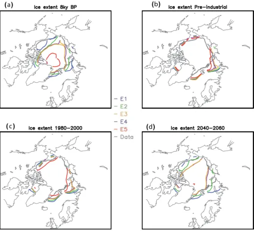
(a) (b)

(d) (c)

Fig. 2. Location of the sea ice edge in September, defined as the 15% ice concentration limit for (a) 8 kyr BP, (b) pre-industrial conditions, (c) the period 1980–2000 AD and (d) the period 2040–2060 AD in scenario SRES B1. E1 is in blue, E2 in green, E3 in orange, E4 in violet

and E5 in red. The observed ice edge for the period 1980–2000 AD (Comiso et al., 1999 and updated 2005) is in grey in all the figures for an easier reference. For the periods 1980–2000 and 2040–2060, the mean over the 5 ensemble members using the same parameter set is presented. For pre-industrial and early Holocene, a 100 year mean is displayed.

cause of a memory effect related to the summer warming, a small winter warming is simulated there (Renssen et al., 2005). However, this warming is too small to induce signifi-cant changes in ice extent.

In contrast to satellite data or model results, proxy records do not directly provide information about the location of the ice edge or about the total sea ice extent. They rather al-low estimating the presence or absence of ice (and in some case the ice concentration or the duration of the ice covered period) at a particular point where the proxy data are col-lected (e.g., Nørgaard-Pedersen et al., 1998; de Vernal and Hillaire Marcel, 2000; Bennike, 2004). On the other hand, models have clear and systematic regional biases as briefly discussed above, making in some area the analysis of re-gional changes questionable. Any model-data comparison related to changes in the ice cover should thus be performed with caution. The available proxy records suggest a reduced summer ice cover and higher oceanic temperatures for the period around 8 kyr BP, but with regional differences. Such a warming and reduced ice cover appears relatively clearly in Baffin Bay and in the Labrador Sea (e.g. Levac et al.,

2001; de Vernal and Hillaire-Marcel, 2006). In the Norwe-gian, Greenland and Barents Seas, the majority of the records also suggest milder conditions during the early Holocene (e.g. Koc¸ et al., 1993; Duplessy et al., 2001; Bennike, 2004), although some studies estimate that the changes were rela-tively small in some parts of the Barents Sea (Voronina et al., 2001) and even that more ice was present at some lo-cations along the eastern coast of Greenland (e.g., Bennike, 2004; Solignac et al., 2006). In addition, the few available observations in the central Arctic suggest a higher amount of open water (leads) during this period (Nørgaard-Pedersen et al., 1998). Besides, in the western Arctic Ocean, the changes appear smaller than in the European sector, with probably a slightly more extensive ice cover in some areas at 8 kyr BP than during recent times (Dyke et al., 2001; de Vernal et al., 2005). In the Labrador and Barents Seas, experiments E1 and E2 thus likely overestimate the summer ice extent at 8 kyr BP, but the discrepancy is of the same order of magnitude as the one observed for present-day conditions. The model-data comparison for 8 kyr BP in this area brings thus only very limited additional information compared to classical

evalua-H. Goosse et al.: Summer sea ice during the early Holocene 687

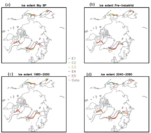
(a) (b)

(d) (c)

Fig. 3. Same as Fig. 2 for the sea ice edge in March.

Table 2. Minimum sea ice extent (in 106km2) in the Northern Hemisphere for different periods.

Name Min ice extent1 preind

Min ice extent 8 BP

Min ice extent 1980–2000

Min ice extent 2040–20603

Trend over the period 1979–20064

Trend over the period 1953–20064 E1 9.4 5.44 9.0 7.65 −0.019±0.008 −0.013±0.005 E2 8.8 3.24 7.79 5.46 −0.041±0.014 −0.019±0.004 E3 8.0 2.08 6.80 3.01 −0.038±0.021 −0.023±0.007 E4 8.5 1.96 7.06 2.92 −0.064±0.020 −0.032±0.017 E5 7.4 0.62 4.76 0.36 −0.087±0.030 −0.063±0.011 Observations2 7.2 −0.060±0.010 −0.051± 0.004

1_{. Ice extent is defined as the total oceanic area with an ice concentration of at least 15%.} 2_{Based on Stroeve et al. (2007).}

3_{In this experiment, scenario SRES B1 is used.}

4_{This represents the mean trend over the ensemble performed for each parameter set (in 10}6_km2_{per decade). The uncertainty is measured} as one standard deviation of the ensemble.

tion of model performance over the last decades. Similarly, in the Greenland Sea in summer and in all regions in win-ter, the differences between the experiments are too weak to discriminate between the behaviour of the experiments, mak-ing the model-data comparison there of limited use in deter-mining the most suitable choice of the parameter sets. An exception is probably experiment E5 in the Greenland Sea for which the absence of ice in summer is likely not realis-tic. However, the discrepancy between proxy data and the results of E5 is much clearer in the western Arctic Ocean,

north of Alaska and of the Canadian Archipelago where ex-periment E5 simulates no ice in summer in opposition with the proxy records. We can thus state that the summer ice cover obtained in this experiment is not consistent with the available proxy-based reconstruction around 8 kyr BP. On the other hand, none of E1–E4 can clearly be rejected on the basis of 8 kyr BP reconstructions.

Fig. 4. Time evolution of the minimum ice extent in the Arctic over

the period 1900–2100 AD using scenario SRES B1. Each simula-tion is represented by a dashed line, while the mean over the 5 sim-ulations with the same parameter set is represented by a solid line of the same colour. The observations (Stroeve et al., 2007) are in black. A 11-year running mean has been applied to the time series.

All the simulations display a decrease in summer sea ice extent throughout the 20th and 21st centuries but with very different magnitudes (Figs. 2, 4). In fact, the range covered by our simulations over this period is even larger than the one given by the IPCC AR4 (Stroeve et al., 2007). Our simula-tions performed with different model parameter sets provide thus a good sample of the present uncertainties in future pro-jections. Compared to observations covering the second half of the 20th century and the beginning of the 21st century, E1, E2 and, to a smaller extent, E3 seriously underestimate the decline in summer ice extent (Table 2). The size of the ensemble of simulations performed for each parameter set is still too small to obtain reliable statistics of internal variabil-ity. Nevertheless, the simulated mean trend is smaller than the observed trend for the period 1953–2006 AD by more than 2 standard deviations over the ensemble, for those three parameters sets (Table 2). We thus consider the eventuality that the observed decline was due to a rare event of natural variability as highly unlikely and we prefer the more reason-able hypothesis that E1 and E2 are incompatible with the ob-served record. In winter, all the simulations also display a decrease in ice extent (Fig. 3). For instance, in E5 the winter ice extent around 2050 using scenario SRES B1 is smaller than during pre-industrial times by 2×106km2. However, this decrease is smaller than in summer and distributed over a longer ice edge, making the local differences in March less clear than for September.

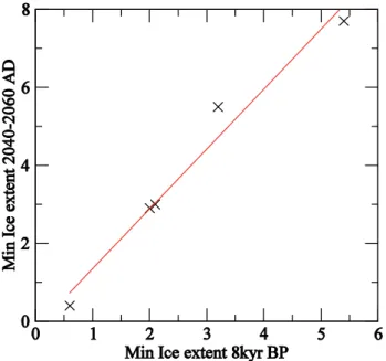
Figures 2 and 4 suggest evidence of strong consistency between past and future summer sea ice changes across the

different parameter sets. Specifically, the summer ice extent averaged over the period 2040–2060 AD is very close to 1.5 times the one simulated for 8 kyr BP for all the model param-eter sets (Fig. 5). As sea ice almost disappears in summer after 2050 AD for E5, the comparison becomes meaningless for this parameter set, but the strong relationship with the ice extent simulated at 8 kyr BP appears also valid for the aver-aged ice extent over the periods 2060–2080 AD and 2080– 2100 AD (not shown).

4 Discussion and conclusions

Only a few reconstructions of the summer sea ice extent are available for the early Holocene. Furthermore, several records could not be efficiently used in the present frame-work because of the too small differences between the sim-ulations at the locations where the proxy data were obtained or because of the inability of the model to reproduce some regional features.

However, the reconstructions still allowed us to show that the model results for one of our parameter sets (E5) are not in agreement with observations, as the summer sea ice cover nearly disappears under early Holocene conditions in this ex-periment. The comparison for 8 kyr BP provides thus an up-per limit on the model sensitivity, allowing the rejection of parameters sets corresponding to too strong a response of the summer ice cover to changes in the radiative forcing. In addi-tion, the analysis of the simulated decrease in ice extent over the last decades shows that simulations presenting a weak response are not compatible with the observed decline of the summer ice extent during this period (E1, E2 and to a smaller extent E3).

From this complementary evidence, the projection ob-tained using the remaining parameter set (E4) appears the most reliable. For the relatively moderate scenario SRES B1, this E4 simulation displays a reduction in summer sea ice extent larger than 60% in 2050 and a nearly disappear-ance of the summer Arctic ice pack at the end of the 21st century. For a more pessimistic scenario like SRES A2, in which the atmospheric CO2concentration in the atmosphere reaches about 830 ppmv in 2100, the decline of the Arctic sea ice in summer would be even faster. Consequently, the Arctic would become almost ice-free in summer in 2060 AD in this scenario (Fig. 6). Those values are below the range (multimodel mean ±1 standard deviation) provided by the IPCC AR4 (Meehl et al., 2007), indicating that this recent report may provide too conservative projections of the future changes in summer sea ice extent for the Arctic. Note that using parameter set E3, which is the second most reliable ac-cording to our analysis, would provide projections relatively similar to the ones obtained using E4 (Figs. 3 and 5).

The strong link between the simulated decrease in the Arctic summer sea ice extent during the 21st century and 8 kyr BP used here to constrain the model behaviour is ob-tained for a wide range of model responses despite the very

H. Goosse et al.: Summer sea ice during the early Holocene 689

Fig. 5. Link between the minimum Arctic sea ice extent (in 106km2) for the early Holocene and the period 2040–2060 AD us-ing scenario SRES B1. Simulations correspondus-ing to different pa-rameter sets (E1 to E5) are represented by a cross. The red line is a regression line for those five points.

different forcings changes during the two periods. Indeed, the forcing is slowly varying in the early Holocene and has a very strong seasonal cycle. By contrast, the forcing changes rapidly over the 20th and 21st centuries, the climate system being in a clearly transient state, and the forcing anomaly is more homogenously distributed for the different seasons. However, we use only a limited number of experiments and only one single model. Additional simulations with LOVE-CLIM using different parameter sets as well as experiments with other coupled climate models would thus be required to test the robustness of the nearly perfect correlation described in Fig. 5. Furthermore, with a larger ensemble of simula-tions, it would be possible to assign to each parameter set a quantitative estimate of its ability to simulate the observed changes in summer ice extent and then provide a probabil-ity distribution for the projected changes instead of simply selecting the most reliable projection as proposed here. In any case, our results strongly suggest that information about the state of the climate system during the early Holocene could help us in reducing our uncertainties on the future de-cline of the summer Arctic ice cover. Additional observa-tions over this period, such as the ones planned in the frame-work of the International Polar Year (e.g.,http://classic.ipy. org/development/eoi/details.php?id=786), are thus required in order to obtain more precise and more reliable projec-tions. Following our experiments, proxy-based estimates of the summer ice cover for the central Arctic, off the shelves of the Kara and Laptev Sea as well as in the Beaufort Sea would provide the strongest tests for model results and observations

Fig. 6. Time evolution of the minimum ice extent in the Arctic over

the period 1900–2100 AD using scenario SRES A2. Each simula-tion is represented by a dashed line while, the mean over the 5 sim-ulations with the same parameter set is represented by a solid line of the same colour. The observations (Stroeve et al., 2007) are in black. A 11-year running mean has been applied to the time series.

in this area would then be particularly useful. Furthermore, simulation for 8 kyr BP should become a standard benchmark for models aiming at providing projections of the evolution of the summer ice extent. Indeed, the summer ice extent in E5, which was rejected here on the basis of the model-data comparison for the Early Holocene, is 0.62 km2at 8 kyr while, in this experiment, the summer sea ice extent reaches 4.8×106km2at 6 kyr BP, i.e. a value very close to the mean for the period 1980–2000 AD (Table 2). This demonstrates that the signal is much stronger at 8 kyr BP than for the more classical 6 kyr BP simulation, providing a much stronger con-straint for the model.

Appendix A

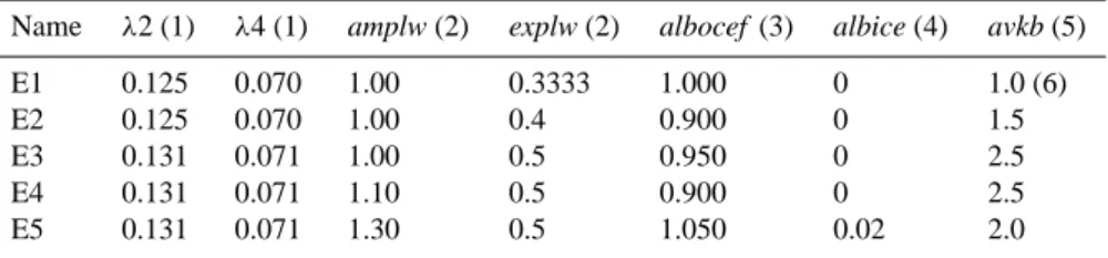
Table A1. The five model parameter sets selected.

Name λ2 (1) λ4 (1) amplw (2) explw (2) albocef (3) albice (4) avkb (5)

E1 0.125 0.070 1.00 0.3333 1.000 0 1.0 (6)

E2 0.125 0.070 1.00 0.4 0.900 0 1.5

E3 0.131 0.071 1.00 0.5 0.950 0 2.5

E4 0.131 0.071 1.10 0.5 0.900 0 2.5

E5 0.131 0.071 1.30 0.5 1.050 0.02 2.0

(1) λ2 and λ4 are two Rossby radii of deformation, applied in the Rayleigh damping term of the equation of the quasi-geostrophic potential vorticity. λ2 corresponds to the 500–800 hPa layer of the model, while λ4 corresponds 200–500 hPa layer (see Eq. (1) of Opsteegh et al., 1998, and Eq. (11) of Haarsma et al., 1996).

(2) The simple longwave radiative scheme of LOVECLIM is based on an approach termed the Green’s function method (Chou and Neelin, 1996; Schaeffer et al., 1998). The scheme could be briefly represented for clear-sky conditions by the following formula for all the model levels:

F lw=F ref +F G(T′, GH G′)+G1 ∗ amplw ∗ (q′) ∗ ∗explw (A1)

where Flw is the longwave flux, Fref a reference value of the flux when temperature, humidity and the concentrations of greenhouse gases are equal to the reference values, FG a function, not explicitly described here, allowing to compute the contribution associated with the anomalies compared to this reference in the vertical profile of temperature (T′) and in the concentrations of the various greenhouse gases in the atmosphere (GHG’). The last term represents the anomaly in the longwave flux due to the anomaly in humidity q′. The coefficients Fref, G1 and those included in the function FG are spatially dependent. All the terms have been calibrated to follow as closely as possible a complex general circulation model longwave scheme (Schaeffer et al., 1998), but large uncertainties are of course related to this parameterization, in particular as the model only computes one mean relative humidity between the surface and 500 hPa, the atmosphere above 500 hPa being supposed to be completely dry.

(3) The albedo of the ocean in LOVECLIM depends on the season and location. At each time step, it is multiplied by albcoef in the experiments analysed here. For a typical albedo of the ocean of 0.06, using a value of 1.05 for albcoef increases the value of the albedo to 0.063.

(4) The albedo of sea ice is based on the scheme of Shine and Henderson-Sellers (1985), which uses different values for the albedo of dry snow, melting snow, frozen ice and melting ice. For thin ice, the albedo is also dependent on the ice thickness. If albice is different from zero in the experiments discussed here, the value of the albedo in the model is increased by albice for all the snow and ice types.

(5) As explained in detail in Goosse et al. (1999), the minimum vertical diffusivity in the ocean follows a vertical profile similar to the one proposed in Bryan and Lewis (1979). The coefficient avkb is a scaling factor that multiplies the minimum values of the vertical diffusivity at all depths. A value of avkb of 1 (1.5, 2, 2.5) corresponds to a minimum background vertical diffusivity in the thermocline of 10−5m2/s (1.510−5, 2 10−5, 2.5 10−5m2/s).

(6) In LOVECLIM1.1, the Coriolis term in the equation of motion is computed in a totally implicit way because the semi-implicit scheme used for this term in LOVECLIM1.0 induced too much numerical noise. The older scheme has been kept here in E1 only, in order to have an easier comparison with the results of LOVECLIM1.0. Because of the larger implicit diffusion associated with this scheme, a lower value of the explicit diffusion is applied in E1.

Acknowledgements. H. Goosse is Research Associate with the

Fonds National de la Recherche Scientifique (FNRS-Belgium). This work is supported by the FNRS and by the Belgian Federal Science Policy Office, Research Program on Science for a Sus-tainable Development. We would like to thank M. Crucifix for his help in the experimental design and for a careful reading of the manuscript, V. Brovkin for his collaboration during the develop-ment of LOVECLIM 1.1, J. Stroeve for sending us the time series of changes in ice extent over the last 30 y as well as A. de Vernal and an anonymous Referee for their helpful comments on an earlier version of the manuscript.

Edited by: P. Braconnot

References

Arzel, O., Fichefet, T., and Goosse, H.: Sea ice evolution over the 20th and 21st centuries as simulated by current AOGCM, Ocean Model., 12, 401–415, 2006.

Bennike, O.: Holocene sea-ice variations in Greenland: onshore evidence, Holocene, 14, 607–613, 2004.

Berger A. L.: Long-term variations of daily insolation and Quater-nary climatic changes, J. Atmos. Sci., 35, 2363–2367, 1978. Braconnot P., Otto-Bliesner, B., Harrison, S., Joussaume, S.,

Pe-terchmitt, J.-Y., Abe-Ouchi, A., Crucifix, M. , Driesschaert, E., Fichefet, Th., Hewitt, C. D., Kageyama, M., Kitoh, A., Loutre, M.-F. , Marti, O., Merkel, U., Ramstein, G., Valdes, P., Weber, S.-L., Yu, Y., and Zhao ,Y.: Results of PMIP2 coupled simula-tions of the Mid-Holocene and Last Glacial Maximum Part 2:

H. Goosse et al.: Summer sea ice during the early Holocene 691 feedbacks with emphasis on the location of the ITCZ and

mid-and high latitudes heat budget, Clim. Past, 3, 279–296, 2007, http://www.clim-past.net/3/279/2007/.

Brovkin, V., Bendtsen, J., Claussen, M., Ganopolski, A., Ku-batzki, C., Petoukhov, V., Andreev, A.: Carbon cycle, veg-etation and climate dynamics in the Holocene: experiments with the CLIMBER-2 model, Global Biogeochem. Cy., 16, doi:10.1029/2001GB001662, 2002.

Bryan, K. and Lewis, L. J.: A water mass model of the world ocean, J. Geophys. Res., 84, 2503–2517, 1979.

Chou, C. and Neelin, J. D.: Linearization of a long-wave radiation scheme for intermediate tropical atmospheric model, J. Geophys. Res., 101, 15 129–15 145, 1996.

Comiso, J.: Bootstrap sea ice concentrations for NIMBUS-7 SMMR and DMSP SSM/I, June to September 2001, Boulder, CO, USA, National Snow and Ice Data Center Digital media, 1999 updated 2005.

Crucifix, M.: Does the Last Glacial Maximum constrain climate sensitivity?, Geophys. Res. Lett., 33, L18701, doi:10.1029/2006GL027137, 2006.

de Vernal, A. and Hilaire-Marcel, C.: Sea-ice cover, sea-surface salinity and halo-thermocline structure of the northwest North Atlantic: modern versus full glacial conditions, Quaternary Sci. Rev., 19, 65–85, 2000.

de Vernal, A., Hilaire-Marcel, C. and Darby, D. A.: Vari-ability of the ice cover in the Chukchi Sea (western Arctic Ocean) during the Holocene, Paleoceanography, 20, PA4018, doi:10.1029/2005PA001157, 2005.

de Vernal, A. and Hilaire-Marcel, C.: Provincialism in trends and high frequency changes in the northwest North Atlantic during the Holocene, Global Planet. Change., 54, 263–290, 2006. Driesschaert, E., Fichefet, T., Goosse, H., Huybrechts, P., Janssens,

I., Mouchet, A., Munhoven, G., Brovkin, V., and Weber, S. L.:Modeling the influence of Greenland ice sheet melt-ing on the Atlantic meridional overturnmelt-ing circulation dur-ing the next millennia, Geophys. Res. Lett., 34, L10707, doi:10.1029/2007GL029516, 2007.

Duplessy, J. C., Ivanova, E., Murdmaa, I., Paterne, M., and Labeyrie L.: Holocene paleoceanography of the northern Barents Sea and variations of the northward heat transport by the Atlantic Ocean, Boreas, 30, 2–16, 2001.

Dyke, A.S. and Savelle, J. M.: Holocene history of the Bering Sea bowhead whale (Balaena mysticetus) in its Beaufort Sea sum-mer grounds off southwestern Victoria Island, western Canadian Arctic, Quaternary Res., 55, 371–379, 2001.

Flato, G. M.: Sea-ice and its response to CO2forcing as simulated by global climate models, Clim. Dynam., 23, 229–241, 2004. Goosse, H. and Fichefet, T.: Importance of ice-ocean interactions

for the global ocean circulation: a model study, J. Geophys. Res., 104, 23 337–23 355, 1999.

Goosse, H., Renssen, H. Timmermann, A., and Bradley, R. S.: In-ternal and forced climate variability during the last millennium: a model-data comparison using ensemble simulations, Quaternary Sci. Rev., 24, 1345–1360, 2005.

Goosse, H., Deleersnijder, E., Fichefet, T., and England, M. H.: Sensitivity of a global coupled ocean-sea ice model to the pa-rameterization of vertical mixing, J. Geophys. Res., 104, 13 681– 13 695, 1999.

Haarsma, R. J., Selten, F. M., Opsteegh, J. D., Lenderink, G., and

Liu, Q.: ECBILT, a coupled atmosphere ocean sea-ice model for climate predictability studies, KNMI, De Bilt, The Netherlands, 31 pp., 1996.

Holland, M. M. and Bitz, C. M.:Polar amplification of climate change in coupled models, Clim. Dynam., 21, 221–232, 2003. Holland, M. M., Bitz, C. M., and Tremblay, B.: Future abrupt

re-ductions in the summer Arctic sea ice, Geophys. Res. Let., 33, L23503, doi:10.1029/2006GL028024, 2006.

Koc¸, N., Jansen, E., and Haflidason, H.: Paleoceanographic recon-structions of surface ocean conditions in the Greenland, Iceland and Norwegian seas through the last 14 ka based on diatoms, Quaternary Sci. Rev., 12, 115–140, 1993.

Lemke, P., Ren J., Alley R. B., et al.: Observations: Changes in Snow, Ice and Frozen Ground, in: Climate Change 2007: The Physical Science Basis, Contribution of Working Group I to the Fourth Assessment Report of the Intergovernmental Panel on Climate Change, edited by: Solomon, S., Qin, D., Manning, M., Chen,Z., Marquis, M., Averyt, K. B., Tignor, M., and Miller, H. L., Cambridge Univ. Press, Cambridge, 2007.

Levac, E., de Vernal, A., and Blabe, W.: Sea-surface conditions in northernmost Baffin Bay during the Holocene : palynological evidence, J. Quaternary Sci., 16, 353–363, 2001.

Masson-Delmotte, V., Kageyama, M., Braconnot, P., Charbit, S., Krinner, G., Ritz, C., Guilyardi, E., Jouzel, J., Abe-Ouchi, A., Crucifix, M., Gladstone, R. M., Hewitt, C. D., Kitoh, A., LeGrande, A. N., Marti, O., Merkel, U., Motoi, T., Ohgaito, R., Otto-Bliesner, B., Peltier, W. R., Ross, I., Valdes, P. J., Vettoretti, G., Weber, S. L., Wolk, F., and Yu, Y.: Past and future polar am-plification of climate change: climate model intercomparisons and ice-core constraints, Clim. Dynam., 27, 437–440, 2006. Meehl, G. A., Stocker, T. F., Collins, W. D., et al.: Global Climate

Projections, in: Climate Change 2007: The Physical Science Basis. Contribution of Working Group I to the Fourth Assess-ment Report of the IntergovernAssess-mental Panel on Climate Change, edited by: Solomon, S., Qin, D., Manning, M., Chen, Z., Mar-quis, M., Averyt, K. B., Tignor, M., and Miller, H. L., Cambridge Univ. Press, Cambridge, 2007.

Murphy, J. M, Sexton, D. M. H., Barnett, D. N., Jones, G. S., Webb, M. J., Collins, M., and Stainforth D. A.: Quantification of mod-elling uncertainties in a large ensemble of climate change simu-lations, Nature, 430, 768–772, 2004.

Nørgaard-Pedersen, N., Spielhagen, R. F., Thiede, J., and Kassens, H.: Central Arctic surface ocean environment during the past 80 000 years, Paleoceanography, 13, 193–204, 1998.

Opsteegh, J. D., Haarsma, R. J., Selten, F. M., and Kattenberg, A.: ECBILT: A dynamic alternative to mixed boundary conditions in ocean models, Tellus, 50A, 348–367, 1998.

Renssen, H., Goosse, H., Fichefet, T., Brovkin, V., Driesschaert,E., and Wolk, F.:Simulating the Holocene climate evolution at north-ern high latitudes using a coupled atmosphere-sea ice-ocean-vegetation mode, Clim. Dynam., 24, 23–43, 2005.

Ridley, J., Lowe, J., Brierley, C., and Hariris, G.: Uncertainty in the sensitivity of Arctic sea ice to global warming in a per-turbed parameter climate model ensemble, Geophys. Res. Lett., 34, L19704, doi:10.1029/2007GL031209, 2007.

Schaeffer, M., Selten, F., and van Dorland, R.: Linking Image and ECBILT, National Institute for public health and the environment (RIVM), Bilthoven, The Netherlands, Report no. 4815008008, 1998.

Schiermeier, Q.: The new face of the Arctic, Nature, 446, 133–135. 2007.

Serreze, M. C., Holland, M. M., and Stroeve, J.: Perspectives on the Arctic’s shrinking sea-ice cover, Science, 315, 1533–1536, 2007. Shine, K. P. and Henderson-Sellers, A.: The sensitivity of a thermo-dynamic sea ice model to changes in surface albedo parameriza-tion, J. Geophys. Res., 90, 2243–2250, 1985.

Solignac, S., Giraudeau, J., and de Vernal A.: Holocene sea surface conditions in the western North Atlantic : spatial and temporal heterogeneities, Paleocenography, 21, PA2004, doi:10.1029/2005PA001175, 2006.

Stainforth, D. A., Aina, T., Christensen, C., Collins, M., Faull, N., Frame, D. J., Kettleborough, J. A., Knight, S., Martin, A., Mur-phy, J. M., Piani, C., Sexton, D., Smith, L. A., Spicer, R. A., Thorpe, A. J., and Allen, M. R.: Uncertainty in predictions of

the climate response to rising levels of greenhouse gases, Nature 433, 403–406, 2005.

Stroeve, J., Holland, M. M., Meier, W., Scambos, T., and Serreze, M.: Arctic sea ice decline: Faster than forecast, Geophy. Res. Lett., 34, L09501, doi:10.1029/2007GL029703, 2007.

Vavrus, S. and Harrison, S.P.: The impact of sea-ice dynamics on the Arctic climate system, Clim. Dynam., 20, 741–757, 2003. Voronina, E., Polyak, L., de Vernal, A., and Peyron O.: Holocene

variations of sea-surface conditions in the southeastern Barents Sea, reconstructed from dinoflagellate cyst assemblages, J. Qua-ternary Sci., 16, 717–726, 2001.

Zhang, X. and Walsh, J. E.:Toward a seasonally ice-covered Arc-tic Ocean: scenarios from the IPCC AR4 model simulations, J. Climate, 19, 1730–1747, 2006.