HAL Id: hal-02134054
https://hal.archives-ouvertes.fr/hal-02134054
Submitted on 15 Dec 2020
HAL is a multi-disciplinary open access
archive for the deposit and dissemination of
sci-entific research documents, whether they are
pub-lished or not. The documents may come from
teaching and research institutions in France or
abroad, or from public or private research centers.
L’archive ouverte pluridisciplinaire HAL, est
destinée au dépôt et à la diffusion de documents
scientifiques de niveau recherche, publiés ou non,
émanant des établissements d’enseignement et de
recherche français ou étrangers, des laboratoires
publics ou privés.
Predictions of the WFIRST Microlensing Survey. I.
Bound Planet Detection Rates
Matthew Penny, B Gaudi, Eamonn Kerins, Nicholas Rattenbury, Shude Mao,
Annie Robin, Sebastiano Calchi Novati
To cite this version:
Matthew Penny, B Gaudi, Eamonn Kerins, Nicholas Rattenbury, Shude Mao, et al.. Predictions of the
WFIRST Microlensing Survey. I. Bound Planet Detection Rates. Astrophysical Journal Supplement,
American Astronomical Society, 2019, 241 (1), pp.3. �10.3847/1538-4365/aafb69�. �hal-02134054�
Typeset using LATEX twocolumn style in AASTeX61
PREDICTIONS OF THE WFIRST MICROLENSING SURVEY I: BOUND PLANET DETECTION RATES
MATTHEWT. PENNY,1B. SCOTTGAUDI,1EAMONNKERINS,2NICHOLASJ. RATTENBURY,3 SHUDEMAO,4, 5, 2ANNIEC. ROBIN,6 ANDSEBASTIANOCALCHINOVATI7
1Department of Astronomy, The Ohio State University, 140 W. 18th Avenue, Columbus, OH 43210, USA
2Jodrell Bank Centre for Astrophysics, Alan Turing Building, University of Manchester, Manchester M13 9PL, UK 3Department of Physics, University of Auckland, Private Bag 92019, Auckland, New Zealand
4Physics Department and Tsinghua Centre for Astrophysics, Tsinghua University, Beijing 100084, China
5National Astronomical Observatories, Chinese Academy of Sciences, A20 Datun Rd., Chaoyang District, Beijing 100012, China
6Institut Utinam, CNRS UMR 6213, OSU THETA, Universit´e Bourgogne-Franche-Comt´e, 41bis avenue de l’Observatoire, F-25000 Besanc¸on, France 7IPAC, Mail Code 100-22, Caltech, 1200 East California Boulevard, Pasadena, CA 91125, USA
(Dated: August 9, 2018) ABSTRACT
The Wide Field InfraRed Survey Telescope (WFIRST) is the next NASA astrophysics flagship mission, to follow the James Webb Space Telescope(JWST). The WFIRST mission was chosen as the top-priority large space mission of the 2010 astronomy and astrophysics decadal survey in order to achieve three primary goals: to study dark energy via a wide-field imaging survey, to study exoplanets via a microlensing survey, and to enable a guest observer program. Here we assess the ability of the several WFIRST designs to achieve the goal of the microlensing survey to discover a large sample of cold, low-mass exoplanets with semimajor axes beyond roughly one AU, which are largely impossible to detect with any other technique. We present the results of a suite of simulations that span the full range of the proposed WFIRST architectures, from the original design envisioned by the decadal survey, to the current design, which utilizes a 2.4-m telescope donated to NASA. By studying such a broad range of architectures, we are able to determine the impact of design trades on the expected yields of detected exoplanets. In estimating the yields we take particular care to ensure that our assumed Galactic model predicts microlensing event rates that match observations, consider the impact that inaccuracies in the Galactic model might have on the yields, and ensure that numerical errors in lightcurve computations do not bias the yields for the smallest mass exoplanets. For the nominal baseline WFIRST design and a fiducial planet mass function, we predict that a total of∼1400 bound exoplanets with mass greater than ∼0.1 M⊕should be detected, including∼200 with mass .3 M⊕. WFIRST should have sensitivity to planets with mass down to∼0.02 M⊕, or roughly the mass of Ganymede.
1. INTRODUCTION
The study of the demographics of exoplanets, the end re-sult of the planet formation process, has entered a statistical age. Large samples of transiting planets from Kepler (e.g., Thompson et al. 2018), massive planets at small to moder-ate separations from ground-based radial velocity surveys of planetary systems in the solar neighborhood (e.g.,Udry & Santos 2007; Winn & Fabrycky 2015), and direct imaging studies of young planets at large separations (e.g., Bowler 2016), are beginning to reveal the complex distribution of exoplanets as a function of mass and separation from their host stars, and the properties of the host stars themselves.
Data from the Kepler mission has revealed a sharp rise in the occurrence rate of hot and warm planets as radius
decreases down to about 2.8R⊕, before leveling off (e.g.,
Howard et al. 2010; Fressin et al. 2013). Precise spectro-scopic measurements of Kepler’s super Earth hosts has re-vealed a radius dichotomy between large and small super Earths (Fulton et al. 2017) that is likely due to atmospheric stripping (Owen & Wu 2017). At large orbital distances &10 AU, direct imaging searches have found young, mas-sive planets to be present, but rare (e.g., Nielsen & Close 2010;Chauvin et al. 2015;Bowler et al. 2015). However, there remains a large area of the exoplanet parameter space – orbits beyond∼1 AU and masses less than that of Jupiter – that remains relatively unexplored by transit, radial velocity, and direct imaging techniques.
Indeed, if every planetary system resembled our own, only a handful of planets would have been discovered by the radial velocity, transit, or direct imaging techniques to date. This fact begs the question: Is our solar system architecture rare? If so, why?
To obtain a large sample of exoplanets beyond 1 AU and across a large range of masses requires a different technique. Gravitational microlensing enables a statistical survey of ex-oplanet populations beyond 1 AU, because its sensitivity peaks at the Einstein radius of its host stars (Mao & Paczyn-ski 1991;Gould & Loeb 1992;Bennett & Rhie 1996). For stars along the line of sight to the Galactic bulge (where the microlensing event rate is highest) the physical Einstein ra-dius is typically2–3 AU (see, e.g., the review ofGaudi 2012). Thanks to the fact that microlensing is sensitive directly to a planet’s mass and not its light or effect on a luminous body, the techniques sensitivity extends out to all orbital radii be-yond∼1 AU (Bennett & Rhie 2002).
Perhaps the most important reason to perform a large exo-planetary microlensing survey is that it opens up a large new region of parameter space. The history of exoplanet searches has been one of unexpected discoveries. At every turn, when a new area of parameter space has been explored, previously unexpected planetary systems have been found. This process began with the pulsar planets (Wolszczan & Frail 1992) and relatively short-period giant planets discovered by the first precision radial velocity searches sensitive to planets (Mayor & Queloz 1995;Campbell et al. 1988;Latham et al. 1989). As radial velocity surveys’ sensitivities and durations grew, highly eccentric massive planets and low mass Neptunes and “Super Earth” planets were discovered (e.g.,Naef et al. 2001; Butler et al. 2004;Rivera et al. 2005). When originally con-ceived, and with the Solar System as a guide, the Kepler mis-sion aimed to detect potentially habitable Earth-sized planets in∼1 AU orbits around Solar-like stars (Borucki et al. 2003). Were all exoplanet systems like our own, Kepler would have found few or no planets (Burke et al. 2015), and those that it did would have been at the limit of its signal-to-noise ra-tio. This result was obviously preempted by the discovery of hot Jupiters, which demonstrated conclusively that not all planetary systems have architectures like our own. Kepler itself has gone on to discover thousands of planetary sys-tems very unlike ours, including tightly-packed multiplanet systems (e.g.,Lissauer et al. 2011) and circumbinary plan-ets (e.g.,Doyle et al. 2011), to name but a few examples. Even moving into unprobed areas of the host mass parameter space has revealed unexpected systems such as TRAPPIST-1 (Gillon et al. 2016) and KELT-9 (Gaudi et al. 2017). Direct imaging searches have revealed young, very massive plan-ets that orbit far from their hosts (e.g.,Chauvin et al. 2004), the most unusual (from our solar-system-centric viewpoint)
being the four-planet system around HR8799 (Marois et al. 2008,2010).
Despite finding the planetary system that is arguably most similar to our own (the OGLE-2006-BLG-109 Jupiter-Saturn analogs Gaudi et al. 2008; Bennett et al. 2010b), ground-based microlensing surveys too have discovered unexpected systems. For example, microlensing searches have found several massive planets around M-dwarf stars (e.g. Dong et al. 2009) that appear to at least qualitatively contradict the prediction of the core accretion theory that giant planets should be rare around low-mass stars (Laughlin et al. 2004). Measurements of planet occurrence rates from microlensing also superficially appear to contradict previous radial veloc-ity results, although a more careful analysis indicates that the microlensing and radial velocity results are consistent ( Mon-tet et al. 2014; Clanton & Gaudi 2014a,b). Other notable microlensing discoveries include circumbinary planets ( Ben-nett et al. 2016), planets on orbits of∼1–10 AU around com-ponents of moderately wide binary stars (e.g., Gould et al. 2014b; Poleski et al. 2014), planets on wide orbits com-parable to Uranus and Neptune (e.g.,Poleski et al. 2017), and planets orbiting ultracool dwarfs (e.g.Shvartzvald et al. 2017).
Having spent over a decade conducting two-stage survey-plus-follow-up planet searches (see, e.g.,Gould et al. 2010, for a review), microlensing surveys have entered a second generation mode, that relies only on survey observations. The OGLE (Udalski et al. 2015a), MOA (Sako et al. 2007) and three KMTNet telescopes (Kim et al. 2016) span the southern hemisphere and provide continuous high-cadence microlensing observations over tens of square degrees ev-ery night that weather allows. Such global, second geration, pure survey-mode microlensing surveys will en-able the initial promise of microlensing to provide the large statistical samples of exoplanets necessary to study demo-graphics (Henderson et al. 2014a), and have begun to de-liver (Shvartzvald et al. 2016;Suzuki et al. 2016). It has long been recognized (e.g.,Bennett & Rhie 2002;Beaulieu et al. 2008;Gould 2009) that exoplanet microlensing surveys are best conducted from space, thanks to the greater ability to resolve stars in crowded fields and to continuously monitor fields without interruptions from weather or the day-night cy-cle.
WFIRST (Spergel et al. 2015) is a mission conceived of by the 2010 decadal survey panel (Committee for a Decadal Survey of Astronomy and Astrophysics 2010) as its top prior-ity large astrophysics mission. It combines mission propos-als to study dark energy with weak lensing, baryon acous-tic oscillations, and supernovae (Joint Dark Enegry Mission-Omega, JDEM-Mission-Omega, Gehrels 2010), with a gravitational microlensing survey (Microlensing Planet Finder, Bennett et al. 2010a), a near infrared sky survey (Near Infrared Sky
Surveyor,Stern et al. 2010) and a significant guest observer component (Committee for a Decadal Survey of Astron-omy and Astrophysics 2010). The later addition of a high-contrast coronagraphic imaging and spectroscopic technol-ogy demonstration instrument (Spergel et al. 2015) addresses a top medium scale 2010 decadal survey priority as well. In this paper we examine only the microlensing survey compo-nent of the mission.
The structure of the paper is as follows. In Section 2 we describe the WFIRST mission, and each of its design stages. In Section 3we describe the simulations we have performed.Section 4presents the yields of the baseline sim-ulations, whileSection 5considers the effects of various pos-sible changes to the mission design. Section 6discusses the uncertainties that affect our results and how they might be mitigated by future observations, modeling, and simulations. Section 7gives our conclusions.
2. WFIRST
2.1. Goals of the WFIRST Microlensing Survey A primary science objective of the WFIRST mission is to conduct a statistical census of exoplanetary systems, from 1 AU out to free-floating planets, including analogs to all of the Solar System planets with masses greater than Mars, via a microlensing survey. It is in the region of∼1–10 AU that the microlensing technique is most sensitive to planets over a wide range of masses (Mao & Paczynski 1991;Gould & Loeb 1992), and where other planet detection techniques lack the sensitivity to detect low-mass planets within reasonable survey durations or present-day technological limits. How-ever, the1–10 AU region is perhaps the most important re-gion of protoplanetary disks and planetary systems for de-termining their formation and subsequent evolution, and can have important effects on the habitability of planets.
The enhancement in surface density of solids at the water ice line,∼1.5–4 AU from the star, is thought to be critical for the formation of giant planets (Hayashi 1981;Ida & Lin 2004; Kennedy et al. 2006). Nevertheless, all stars do not produce giant planets that survive (e.g., Winn & Fabrycky 2015). It remains to be seen whether this is due to inefficient production of giant planets, or a formation process that is ∼100% efficient followed by an effective destruction mech-anism, such as efficient disk migration (e.g., Goldreich & Tremaine 1980), or ejection or host star collisions caused by dynamics (e.g.Rasio & Ford 1996). In the core accretion sce-nario (e.g.,Goldreich & Ward 1973;Pollack et al. 1996), run-away gas accretion onto protoplanet cores to produce giant planets is an inevitability, if the cores grow large enough be-fore the gas dissipates from the protoplanetary disk (Mizuno 1980). If core growth rate is the rate limiting step in the pro-duction of giant planets, and the process is indeed inefficient, then we can expect a population of “failed cores” of various
masses with a distribution that peaks near the location of the ice line. Conversely, if giant planet formation and subsequent destruction is efficient, we can expect the formed giant plan-ets to clear their orbits of other bodies, and thus would expect to see a deficit of low mass planets in WFIRST’s region of sensitivity.
It is clear that planetary systems are not static, and the or-bits of planets can evolve during and after the planet forma-tion process, first via drag forces while the protoplanetary disk is in place (Lin et al. 1996), and subsequently by N -body dynamical processes once the damping effect of the disk is removed (Rasio & Ford 1996). In addition to rear-ranging the orbits of planets that remain bound, the chaotic dynamics of multiplanet systems can result in planets being ejected (e.g., Safronov 1972). The masses and number of ejected planets from the system will be determined by the number of planets in their original systems, their masses and orbital distribution (e.g,Papaloizou & Terquem 2001;Juri´c & Tremaine 2008;Chatterjee et al. 2008;Barclay et al. 2017). So, the mass function of ejected, or free-floating, planets can be an important constraint on the statistics of planetary sys-tems as a whole. Because they emit very little light, only microlensing observations can be used to detect rocky free-floating planets. For masses significantly below Earth’s, only space-based observations can provide the necessary combi-nation of photometric precision, cadence, and total number of sources monitored in order to collect a significant sample of events.
For both bound and free-floating objects it is valuable to extend the mass sensitivity of an exoplanet survey down past the characteristic mass scales of planet formation the-ory, where the growth behavior of forming planets changes. This is particularly the case for boundaries in mass between low and high growth rates, as these should be the locations of either pile-ups or deficits in the mass function, depending on the sense of the transition. In the core accretion scenario of giant planet formation, moving from high to low masses, characteristic mass scales include the critical core mass for runaway gas accretion at∼10M⊕(Mizuno 1980), the isola-tion mass of planetary embryos at∼0.1M⊕ (Kokubo & Ida 2002), and the transition core mass for pebble accretion at ∼0.01M⊕ (Lambrechts & Johansen 2012). The detection of features due to these characteristic mass scales would be strong evidence in support of current planet formation theory. Additionally, a statistical accounting of planets on wider or-bits more generally will be a valuable test of models of planet formation developed to explain the large occurrence rate of super-Earths closer than 1 AU.
An estimate of the occurrence rate of rocky planets in the habitable zones (e.g., Kasting et al. 1993; Kopparapu et al. 2013) of solar-like stars,η⊕, is an important ingredi-ent for understanding the origins and evolution of life, and
the uniqueness of its development on Earth. However, it is precisely this location that it is both hardest to detect∼1M⊕ planets around∼1M stars, while also remaining tantaliz-ingly achievable. Tiny signals recurring on approximately year timescales mean that transit, radial velocity, and as-trometric searches must run for multiple years to make ro-bust detections. Only the transit technique has demonstrated the necessary precision to date, and even so, Kepler fell just short of the mission duration necessary to robustly measure η⊕(Burke et al. 2015). Direct imaging of habitable exoplan-ets will require significant technological advances (e.g., Men-nesson et al. 2016;Bolcar 2017;Wang et al. 2018), several of which WFIRST’s coronagraphic instrument will demon-strate, in order to reach the contrast and inner working angles required, and the observing time required to perform a blind statistical survey to measureη⊕may be prohibitively expen-sive. The typical inner sensitivity limit for a space-based microlensing survey, which is proportional to the host mass M1/2, crosses the habitable zone, which scales as∼M3.5, at ∼1M . Nevertheless the detection efficiency for low-mass-ratio planets inside the Einstein ring (RE ∼ 3 AU) is very small, and solar-mass stars make up only a small frac-tion of the lens populafrac-tion, so large, long-durafrac-tion microlens-ing surveys from space are required to robustly measureη⊕ with microlensing. In all likelihood, no one technique will prove sufficient, and it will be necessary to combine mea-surements from multiple techniques to be confident in the accuracy ofη⊕determinations. If the habitable zone is ex-tended outward (e.g.,Seager 2013), by volcanic outgassing of of H2(Ramirez & Kaltenegger 2017) or some other pro-cess, the number of habitable planets space-based microlens-ing searches are sensitive to increases significantly.
Each of the goals described above can be addressed in whole or in part by studying the statistics of a large sample of planets with orbits in the range of1–10 AU, and a similar sample of unbound planets. Such a sample can only be deliv-ered by a space-based microlensing survey. Astrometry from Gaiacan be used to discover a large sample of giant planets in similar orbits, but it will not have the sensitivity to probe below∼30M⊕ (Perryman et al. 2014). Space-based transit surveys have sensitivity to very small, and low-mass plan-ets, but would be required to observe for decades to cover the same range of orbital separations as does microlensing. Ground-based microlensing searches have sensitivity to low-mass exoplanets down to∼1M⊕, as recently demonstrated byBond et al.(2017) andShvartzvald et al.(2017), but are limited from gathering large samples of such planets or ex-tending their sensitivity to masses significantly smaller than this by a combination of the more limited photometric pre-cision possible from the ground, the larger angular diameter of source stars for which high precision is possible, and the lower density of such sources on the sky.
A critical element in measuring the mass function of plan-ets from microlensing events is actually measuring planplan-ets masses. The lightcurve of a binary microlensing event alone only reveals information about the mass ratioq, unless the event is long enough to measure the effect of annual mi-crolensing parallax on the lightcurve, or the event is observed from two widely separated observers, e.g., a spacecraft such as Spitzer (e.g.,Udalski et al. 2015b) or Kepler (see Hender-son et al. 2016, for a review). It is also necessary to mea-sure finite source effects in the lightcurve, but this is rou-tinely achieved for almost all planetary microlensing events observed to date, and will likely be possible for the majority of WFIRST’s planetary events (e.g.,Zhu et al. 2014). High resolution imaging enables an alternative method to measure the host and planet mass. Over time, the source and lens star involved in a microlensing event will separate, and the lens, if bright enough will be detectable, either as an elongation in the combined source-lens image, as a shift in the centroid of the pair as a function of color, or if moving fast enough, the pair will become resolvable (e.g.,Bennett et al. 2007). The measured separation between the stars, and the color and magnitude of the lens star can be combined with the measure-ment of the event timescale to uniquely determine the mass of the lens. A principle requirement of the WFIRST mission is the ability to make these measurements routinely for most events. This is made possible by the resolution achievable from space, and is also greatly aided by the fainter source stars that space-based observations enable. For WFIRST to make these measurements it is necessary that it observe the microlensing fields over a time baseline of4 or more years.
In this paper we will only address WFIRST’s ability to measure the mass function of bound planets. The challenges and opportunities to detect free-floating planets, and plan-ets in the habitable zone, differ somewhat from those for the general bound planet population. We have therefore elected to give them the full attention that they deserve in subse-quent papers, rather than provide only the limited picture that would be possible in this paper.
2.2. Evolution of the WFIRST Mission: Design Reference Missions, AFTA, and Cycle 7
The WFIRST mission is in the process of ongoing design refinement, and has gone through four major phases so far. This paper presents analysis of each of these missions, even though some of these designs are no longer under active de-velopment. This is important for two reasons. First, we are documenting the quantitative simulations that have informed the WFIRST microlensing survey design process from the first science definition team. Second, each design represents a internally self consistent set of mission design parameters, that when evolved to a new mission design necessarily cap-tures the majority of covariance between all of the possible
design choices. These covariances are difficult to account for in simulations that might aim to investigate variations in individual parameters that by isolating their effects.
The first WFIRST design, the Interim Design Reference Mission (IDRM) was based directly on the WFIRST mis-sion proposed by the decadal survey and described in the first WFIRST Science Definition Team’s (SDT) interim re-port (Green et al. 2011). This in turn was based on the design for the JDEM-Omega mission (Gehrels 2010). The IDRM consisted of an unobstructed 1.3-m telescope with a 0.294 deg2 near-infrared imaging channel with broadband filters spanning∼0.76 − 2.0 µm, including a wide 1 − 2 µm filter for the microlensing survey, and two slitless spectro-scopic channels.
The final report of the first WFIRST SDT (Green et al. 2012) presented two Design Reference Missions (DRM1 and DRM2). DRM1 was an evolution of the IDRM, adhering to the recommendation of the decadal survey to only use fully developed technologies. It improved on the IDRM by increasing the upper wavelength cutoff of the detectors to 2.4 µm, and removing the two spectroscopic channels. The detectors and prism elements were added to the imag-ing channel to increase its field of view to0.377 deg2.
DRM2 was a design intended to reduce the cost of the mis-sion. This was done by reducing the size of the primary mir-ror to 1.1-m (in order to fit onto a less costly launch vehicle). It also switched to a larger format 4k×4k detector to reduce the number of detectors while increasing the field of view to 0.585 deg2, at the cost of additional detector development. The larger field of view also allowed the mission duration to be shortened to 3 years instead of 5.
The WFIRST design process was disrupted in 2012 when NASA was gifted two 2.4-m telescope mirrors and opti-cal tube assemblies by another government agency. The value of these telescopes to the WFIRST mission was ini-tially assessed in a report byDressler et al.(2012), and the mission designed around one of the 2.4-m telescopes was dubbed WFIRST-AFTA (AFTA standing for Astrophysically Focussed Telescope Assets). A new SDT was assembled to produce an AFTA DRM, which added a coronagraphic in-strument channel to the mission (Spergel et al. 2013). The design of the wide field instrument (WFI) also changed, re-quiring a finer pixel scale to sample the smaller point spread function (PSF) of the2.4-m telescope, and hence a smaller field of view of0.282 deg2. Unlike the previous designs, the telescope has an obstructed pupil, so the PSF has significant diffraction spikes that the previous versions did not. The de-sign also required a shorter wavelength cutoff of2.0 µm due to concerns about the ability to operate the telescope at low temperature required for2.4µm observations. The final re-sults of this design process were presented bySpergel et al. (2015). Z087 W 149 W 169 G2-dwarf AH= 0.00 G2-dwarf AH= 0.66 M5-dwarf AH= 0.66 T h ro u gh p u t (M ir ro rs + D et ec to rs ) Wavelength (µm) IDRM DRM1 DRM2 AFTA Cycle 7 0 0.2 0.4 0.6 0.8 1 0.5 1 1.5 2 2.5 0 0.2 0.4 0.6 0.8 1 0.5 1 1.5 2 2.5
Figure 1. Total throughput curves for each of the mission designs, compared to spectra of stars of different spectral types, suffering differing amounts of extinction. The spectrum of a Teff = 5800 K,
log g = 4.5 G-dwarf taken from the NEXTGEN grid (Hauschildt
et al. 1999) is plotted with no extinction (orange line) and with
AH = 0.66 (gray line), which is typical for the expected WFIRST
fields shown inSection 3.3. G-dwarfs will be the bluest stars that will act as source stars in significant numbers, because more mas-sive stars have evolved off the main sequence in the old bulge pop-ulation. The y-axis units of the spectra are proportional to the pho-tons per unit wavelength (dN/dλ), but each is arbitrarily normal-ized. The throughput curves show the total system throughput in-cluding detector quantum efficiency, and are only shown for the Z087 and W 149 filters. The WFIRST microlensing survey will likely use a wider selection of filters than this.
WFIRST entered the formulation phase (phase A) in early 2016. The AFTA design was adopted, and the mission re-verted to its simpler naming of WFIRST. Extensive design and testing work has been conducted since formulation be-gan. This includes a large amount of detector development, validation of the ability of the telescope to operate cooled, re-design of the wide field instrument, and consideration of var-ious mission descopes. Very recently, WFIRST ended into the second phase of mission development (phase B).
The most significant update to the design affecting the mi-crolensing survey is a more pessimistic accounting of the ob-servatory’s slew time performance compared to the AFTA design. Another important change was a rotation of the elongated detector layout by 90◦. While the mission design continues to evolve, we present simulations here that most closely match the Cycle 7 design, and so throughout the pa-per we will refer to the design as WFIRST Cycle 7.
Table 1summarizes the parameters of each mission design that we study. We use these parameters for the results pre-sented inSection 4andSection 4.1. InSection 5we present the results of “trade-off” simulations that were conducted during the design process, when many of the mission param-eters changed regularly. Between any given set of trade-off simulations, the exact values of many of the simulation
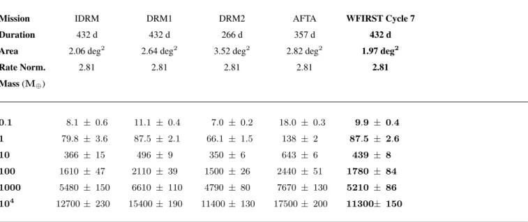
pa-Table 1. Adopted parameters of each mission design
IDRM DRM1 DRM2 AFTA WFIRST Cycle 7
Reference Green et al.(2011) Green et al.(2012) Green et al.(2012) Spergel et al.(2015) —1,2
Mirror diameter (m) 1.3 1.3 1.1 2.36 2.36
Obscured fraction (area, %) 0 0 0 13.9 13.9
Detectors 7×4 H2RG-10 9×4 H2RG-10 7×2 H4RG-10 6×3 H4RG-10 6×3 H4RG-10
Plate scale (“/pix) 0.18 0.18 0.18 0.11 0.11
Field of view (deg2) 0.294 0.377 0.587 0.282 0.282
Fields 7 7 6 10 7
Survey area (degs) 2.06 2.64 3.52 2.82 1.97
Avg. slew and settle Time (s) 38 38 38 38 83.1
Orbit L2 L2 L2 Geosynchronous L2
Total Survey length (d) 432 432 266 411∗∗ 432
Season length (d) 72 72 72 72 72
Seasons 6 6 3.7 6 6
Baseline mission duration (yr) 5 5 3 6 5
Primary bandpass (µm) 1.0–2.0 (W149) 1.0–2.4 (W169) 1.0–2.4 (W169) 0.93–2.00 (W149) 0.93–2.00 (W149) Secondary bandpass (µm) 0.74–1.0 (Z087) 0.74–1.0 (Z087) 0.74–1.0 (Z087) 0.76–0.98 (Z087) 0.76–0.98 (Z087)
W149 Z087 W169 Z087 W169 Z087 W149 Z087 W149 Z087
Zeropoint∗(mag) 26.315 25.001 26.636 24.922 25.990 24.367 27.554 26.163 27.615 26.387
Exposure time (s) 88 116 85 290 112 412 52 290 46.8 286
Cadence 14.98 min 11.89 hr 14.35 min 12.0 hr 15.0 min 12.0 hr 15.0 min 12.0 hr 15.16 min 12.0 hr
Bias (counts/pix) 380 380 1000 1000 1000 1000 1000 1000 1000 1000
Readout noise?(counts/pix) 9.1 9.1 7.6 4.2 9.1 9.1 8.0 8.0 12.12 12.12
Thermal + dark†(counts/pix/s) 0.36 0.36 0.76 0.76 0.76 0.76 1.30 0.05 1.072 0.130
Sky background‡(mag/arcsec2) 21.48 21.54 21.53 21.48 21.52 21.50 21.47 21.50 21.48 21.55
Sky background (counts/pix/s) 2.78 0.79 3.57 0.77 1.99 0.45 3.28 0.89 3.43 1.04
Error floor (mmag) 1.0 1.0 1.0 1.0 1.0 1.0 1.0 1.0 1.0 1.0
Saturation§(103counts/pix) 65.5 65.5 80 80 80 80 679 2037 679 679
Notes: Parameters listed in the table are those used in the main simulations whose results are described in Sections 4 and 5 and are not necessarily the same as described in the relevant WFIRST reports. Where parameters are incorrect, the impact they would have was judged to be too insignificant to justify a repeated run of the simulations with the correct parameters (see text for further justifications). For correct parameter values the reader should refer to the appropriate Science Definition Team (SDT) report, or the reference information currently listed on the WFIRST websites below.
1
https://wfirst.gsfc.nasa.gov/science/WFIRST_Reference_Information.html
2https://wfirst.ipac.caltech.edu/sims/Param_db.html
∗
Magnitude that produces 1 count per second in the detector.
?
Effective readout noise after multiple non-destructive reads. All values are inaccurate, as they depend on the chosen readout scheme. However, the readout noise will not be larger than the correlated double sampling readout noise of ∼20 e−, which is still sub-dominant relative to the combination of zodiacal light and blended stars.
†
Sum of dark current and thermal backgrounds (caused by infrared emission of the telescope and its support structures etc.).
‡
Evaluated using zodiacal light model at a season midpoint; in our simulations we use a time dependent model of the Zodiacal background
(seeAppendix Afor details).
§
Effective saturation level after full exposure time. For the designs preceding AFTA, we assumed saturation would occur when the pixel’s charge reached the full-well depth. For AFTA we assume that, thanks to multiple reads, useful data can be measured from pixels that saturate after two reads, so for a constant full well depth, the saturation level increases with exposure time.
∗∗
rameters changed by small amounts. Rather than tediously detail each of these parameter changes that have little effect on the absolute yields, we will only indicate changes to pa-rameters where they are important to each study. Invariably, these will be the independent variables of each study, or pa-rameters closely related to these. As the unimportant param-eters do not change internal to each trade-study, we compute differential yield measurements, i.e., yields relative to a fidu-cial design.
2.3. The WFIRST Microlensing Survey
The full operations concept for the WFIRST mission must ensure that the spacecraft can conduct all the observations necessary to meet its primary mission requirements, while maintaining sufficient flexibility to conduct a significant frac-tion of potential general observer observafrac-tions. These con-siderations must feed into the spacecraft hardware require-ments while simultaneously being constrained by practical design considerations in an iterative process. An example of an observing time line that results from this process in given in theSpergel et al.(2015) report.
While constructing a sample observing schedule for WFIRSTis a complicated optimization task, requirements set by the nature of microlensing events significantly simplify the process for the microlensing survey. First, the microlens-ing event rate is highly concentrated towards the Galactic bulge, close to the ecliptic. This means that a spacecraft with a single solar panel structure parallel to its telescope’s optical axis can only perform microlensing observations twice per year when the Galactic bulge lies perpendicular to the Sun-spacecraft axis. Second, microlensing events last roughly twice the microlensing timescale tE, with 2tE∼60 d, and planetary deviations last between an hour and a day (see, e.g., Gaudi 2012). This means that a microlensing survey must observe for at least 60 days in order to characterize the whole microlensing event, while also observing at high cadence continually for periods&1 day in order to catch and characterize microlensing events. To operate at maximum efficiency it should continuously observe for the entire dura-tion of its survey windows. Finally, the survey requirement to detect∼100 Earth-mass planets combined with a detec-tion efficiency of∼0.01 per event and a microlensing event rate of a∼few×10−5 yr−1star−1imposes a requirement of monitoring a∼few×108 star years over the duration of the survey.
The duration of planetary deviations places a require-ment on the cadence of the microlensing observations. The timescale of planetary deviations is comparable to the Ein-stein crossing timescale of an isolated lens of the same mass, tE ≈ 2 hr pM/M⊕, and the deviation must be sampled by several data points in order to robustly extract parame-ters. Furthermore, the duration of finite source effects in
the lightcurve, which carry information about the angular Einstein radiusθE, and also need to be resolved by several data points are∼1 hr. Combined, these require an observ-ing cadence of∼15 min. If stars are well resolved, accurate photometry is possible for much of the bulge main sequence in exposures∼1 minute on ∼1 m-class telescopes, and so it should be possible to observe between 5 and 10 fields within the cadence requirements if the observatory can slew fast enough.
The microlensing event rate is highest within a few degrees of the Galactic center, but these regions are also affected by a large amount of extinction. Observations in the near infrared drastically reduce the effect of the extinction. The WFIRST microlensing survey maximizes its photometric precision by using a wide (1–2µm) bandpass for most of its observations, shown inFigure 1. Combining the wide filter with its wide 0.28 deg2 field of view, the current design of WFIRST can monitor a sufficient number of microlensing events with suf-ficient precision with ∼400 days of microlensing observa-tions. Less frequent observations will be taken in more typi-cal broadband filters, here we assumeZ087 in order to mea-sure the colors of microlensing source stars and to meamea-sure color-dependent centroid shifts for luminous lenses when the source and lens separate; the range of intrinsicZ087−W 149 colors of stars is shown inFigure 22inSection A.1. Note that WFIRST magnitudes are on the AB system (Oke & Gunn 1983), and all magnitudes in this paper will be expressed in this system, unless denoted by a subscript Vega.
WFIRST’s microlensing survey therefore looks similar across all designs of the spacecraft, with 72 continuous days of observations occurring around vernal and autum-nal equinoxes. Six of these seasons are required, with three occurring at the start of the mission and three at the end in order to maximize the baseline over which relative source-lens proper motion can be measured (see, e.g.,Bennett et al. 2007). The 2.4 m telescope designs of WFIRST have a smaller field of view than the∼1 m class designs, but can monitor significantly fainter stars at a given photometric precision due to their smaller PSF and larger collecting area, resulting in a similar number of fields being required to reach the same number of stars, despite the difference in field of view. After these two effects cancel, the designs with larger diameter mirrors come out as significantly more capable sci-entifically due to their improvement in ability to measure relative lens-source proper motions.Table 2summarizes the parameters of the latest iteration of the WFIRST microlens-ing survey design and the survey yields that we will describe in later sections.
3. SIMULATING THE WFIRST MICROLENSING SURVEY
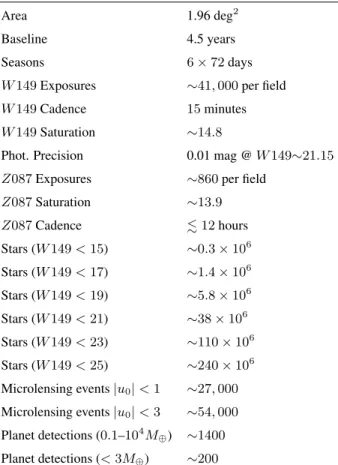
Table 2. The WFIRST Microlensing Survey at a Glance
Area 1.96 deg2
Baseline 4.5 years
Seasons 6 × 72 days
W 149 Exposures ∼41, 000 per field
W 149 Cadence 15 minutes
W 149 Saturation ∼14.8
Phot. Precision 0.01 mag @ W 149∼21.15
Z087 Exposures ∼860 per field
Z087 Saturation ∼13.9 Z087 Cadence . 12 hours Stars (W 149 < 15) ∼0.3 × 10⁶ Stars (W 149 < 17) ∼1.4 × 10⁶ Stars (W 149 < 19) ∼5.8 × 10⁶ Stars (W 149 < 21) ∼38 × 106 Stars (W 149 < 23) ∼110 × 106 Stars (W 149 < 25) ∼240 × 106 Microlensing events |u0| < 1 ∼27, 000 Microlensing events |u0| < 3 ∼54, 000 Planet detections (0.1–104M⊕) ∼1400 Planet detections (< 3M⊕) ∼200
Notes: Assumes the Cycle 7 design. Saturation estimates assumes the brightest pixel accumulates 105 electrons before the first read. Star counts have been corrected for the Besanc¸on model’s under-prediction (see Section 3.2.1). The exposure time and cadence of observations in the Z087 and other filters has not been set; we have assumed a 12 hour cadence here, but observations in the other filters are likely to be more frequent.
We performed our simulations using the GULLScode, of which we only give a brief overview here, and refer the reader toPenny et al.(2013, hereafterP13) for full details.1 In
or-der to fully simulate WFIRST we have made a number of upgrades toGULLS, which are described in the Appendix.
GULLSsimulates large numbers of individual microlensing events involving source and lens stars that are drawn from star catalogs produced by a population synthesis Galactic model. Source stars are drawn from a catalog with a faint magnitude limit (hereHVega = 25), and lens stars from a catalog with no magnitude limit; source lens pairs where the distance of the source is less than the distance of the lens are rejected. Each catalog is drawn from a small solid an-gleδΩ, but represents a larger 0.◦25× 0.◦25 sight line at its specified Galactic coordinates(`, b). The impact parameter
1Note that inP13the software was called MABµLS, but was renamed to
disambiguate it from the MaBµLS online tool (Awiphan et al. 2016).
u0and time of the eventt0are drawn from uniform distribu-tions with limits[−u0,max, +u0,max] and [0, Tsim], respec-tively, whereu0,max= 3 is the maximum impact parameter andTsimis the simulation duration.
Each simulated eventi is assigned a normalized weight wi proportional to its contribution to the total event rate in the sight line
wi= 0.252deg2f1106,W F IRSTΓdeg2Tsimu0,max2µrel,iθE,i
W ,
(1) whereΓdeg2is the event rate per square degree computed via
Monte Carlo integration of the event rate using the source and lens catalogs (seeP13andAwiphan et al. 2016for de-tails),f1106,W F IRST is the event rate scaling factor that we use to scale the event rate computed from the Galactic model to match measured event rates (seeSection 3.2for details), µrel,i is the relative lens-source proper motion of simulated eventi, θE,iis the angular Einstein radius of eventi, and
W =X
i
2µrel,iθE,i (2)
is the sum of un-normalized “event rate weights” for all sim-ulated events in a given sight line. As such, the sum ofwi for all events is simply the number of microlensing events we expect to occur in the sight line during the simulation duration with source stars matching the source catalog’s se-lection criteria. Similarly, the prediction for the number of events matching a given criteria (e.g., a∆χ2 > 160 detec-tion threshold due to a planetary deviadetec-tion) is simply the sum of normalized weights of events that pass the cut, e.g.,
N (∆χ2> 160) =X i
wiH(∆χ2i − 160), (3) whereH(x) is the Heaviside step function.
Binary (planetary) microlensing lightcurves are com-puted using a combination of the hexadecapole approxi-mation (Pejcha & Heyrovsk´y 2009; Gould 2008), contour integration (Gould & Gaucherel 1997;Dominik 1998) and rayshooting (when errors are detected in the contour inte-gration routines, Kayser et al. 1986). Realistic photometry of each event is simulated by constructing images of star fields (drawn from the same population synthesis Galactic model) for each observatory and filter considered, such that the same stars populate images with different pixel scales and filters. The PSF of the baseline source and lens stars are added at the same position on the image. As the event evolves, the source star brightness is updated and photome-try is performed on the image for each data point. For some of the simulations we have implemented a faster photome-try scheme that bypasses the need to create a realization of an image for each data point, and which is described in the Appendix. Figure 2 shows examples of simulated images
Figure 2. Left column: Section of a VVV H band image (Saito et al. 2012) from near (`, b) = (1.◦1, −1.◦2), which lies close to the center of the expected WFIRST fields. Right four columns: Simulated images in the primary wide band of the IDRM, DRM1, DRM2, and AFTA WFIRST designs of the same mock star field drawn from the Besanc¸on model sight line at (`, b) = (1.◦1, −1.◦2). The top panels show a 1×1 arcmin2 region and the bottom panels show a 4.6×4.6 arcsec2 (≈ 13×) zoom-in. The pixel sizes are 0.00
339, 0.0018, 0.0018, 0.0018 and 0.0011 from left to right respectively. Note that the apparent dark, tenuous, serpentine feature on the left side of the simulated images is a result of random fluctuations in the stellar density, and is not due to spatially varying extinction (e.g., a dust lane). The VVV image based on data products from observations made with ESO Telescopes at the La Silla or Paranal Observatories under ESO programme ID 179.B-2002.
Figure 3. Simulated color images of an example bulge field at (`, b) = (0.◦0, −1.◦5) imaged using WFIRST’s Cycle 7 detector, compared with a ground-based observatory based on OGLE’s 1.3-m telescope (e.g.,Udalski et al. 2015a) in optical filters. The WFIRST image is built from a single simulated exposure of 290, 52, and 145 s in Z087, W 149, and F 184 filters, respectively; the OGLE image was built from single simulated exposures of 150, 125, and 100 s in V , R, and I filters, respectively, i.e., typical of the stan-dard OGLE survey exposures. Note the different sizes of the im-ages compared to the previous figure, and that at least some of the WFIRSTfields will be amenable to observations with ground-based optical telescopes.
for IDRM, DRM1, DRM2, and AFTA designs compared to a ground-based IR image, andFigure 3 shows an example simulated color image comparing WFIRST’s performance to a simulated ground-based optical telescope in a field typical for the WFIRST microlensing survey.
Each star is added using realistic numerical PSFs that are integrated over the detector pixels for a range of sub-pixel offsets and stored in a lookup table for rapid access. For IDRM, DRM1 and DRM2, which all have unobstructed aper-tures, we used an Airy function averaged over the band-pass of the filter. For AFTA we used numerical PSFs pro-duced using the ZEMAX software package (D. Content priv. comm.). For the Z087 filter we used the monochromatic PSF computed at 1 µm and for the wide filter we averaged the PSFs computed at1.0, 1.5 and 2.0 µm with equal weights. This crude integration procedure insufficiently samples the changing size of the Airy rings as a function of wavelength, so the resulting PSFs have much more prominent higher-spatial frequency rings than the actual PSF. The real PSF will be much smoother in the wings (see, e.g.,Gould et al. 2014b). The spacing of the unrealistic rings is smaller than the photometric aperture we use, so the inaccurate PSF will have little effect on our results because maxima and minima will average out over the aperture). For the Cycle 7 design we used well sampled numerical PSFs generated using the WEBBPSF tool (Perrin et al. 2012) with parameters from Cycle 5; while the diffraction spikes of these PSFs are
ro-Assumes one 46.8 s exposure/15 min ∼ S at u ra ti on σW 1 4 9 [m ag /1 5 m in ] W 149 0.001 0.01 0.1 1 12 14 16 18 20 22 24 26
Figure 4. Single epoch photometric precision for isolated point sources as a function of magnitude for the Cycle 7 design’s assumed exposure time (46.8 s) assuming no blending. The vertical dashed line indicates the approximate point of saturation in a single read. tated 90 degrees relative to the Cycle 7 design, this has no practical effect on our simulated results.
The capabilities of crowded field photometric techniques are approximated by performing aperture photometry on the image with fixed pointing. We found that a3×3 pixel square aperture produced the best results in the crowded WFIRST fields. This simple photometry scheme enables us to accu-rately simulate all the sources of photon and detector noise that arise in the conversion of photons to data units on an im-age of minimal size. Aperture photometry is sub-optimal in crowded fields, but we can use this fact to compensate for the effect of any un-modeled causes of additional photomet-ric noise resulting from imperfect data analysis (the precision of any method can only asymptotically approach the theoret-ically possible photon noise, and sometimes may be far from it), systematic errors (e.g., we do not simulate pointing shifts or variations in pixel response), or data loss. The resultant photometric precision as a function of magnitude is shown inFigure 4, assuming no blending. Properly simulating all sources of systematic or red noise would require a more de-tailed simulation of the photometry pipeline (for example, by performing difference imaging on images that suffer point-ing shifts) and would be significantly more computationally expensive as a significantly larger image would need to be recomputed for each data point. Rather than do this, we sim-ply add in quadrature a Gaussian systematic error floor to the photometry we measure.
We note that we have not correctly simulated the read out schemes employed by the HAWAII HgCdTe detectors WFIRST will use. Our simulations simulate the CCD read-out process, i.e., an image is exposed for a timetexpbefore being read out pixel by pixel by a one or a small number of amplifiers in a destructive process. Individual pixels in an
infrared HgCdTe array have their own amplifier and can be read out non destructively multiple times per exposure at a chosen rate. HgCdTe amplifiers typically have higher read noise than CCD amplifiers, and so multiple non-destructive reads are employed to reduce the effective read noise in the image. Multiple image “frames” can potentially be stored and downlinked, or processed on-board the spacecraft, en-abling retrieval of useful data from pixels that would saturate in the full exposure time or that get hit by cosmic rays.
Our photometry simulations assume a single readout at the end of an exposure with a gain of1 e−/ADU. The ac-tual gain value will be different, but any digitization uncer-tainty will be small compared to the readout noise. We ap-proximate the effective readout noise in WFIRST images us-ing the erratum correction of the formula given byRauscher et al.(2007), based on the correlated double sampling read-out noise requirements of each design, an assumed readread-out rate, and the exposure time. The full well depth parameter in our simulations is applied to the full exposure time, so we in-crease the detector full well depth requirement by a factor of texp/tread, wheretreadis the time interval between reads of a given pixel, to simulate the ability to extract a measurement from a pixel that does not saturate before the first read. This workaround results in an underestimate of the Poisson noise component of photometry, but the addition of a 0.001 mag systematic uncertainty in quadrature to the final photometric measurement involving 9 pixels prevents a severe underes-timate of the uncertainty in such situations. We note that it should be possible to extract accurate photometry from any pixels that do not saturate before the first read (see Gould et al. 2014a).
To assess whether a simulated event contains a detectable planet we use a simple∆χ2selection criteria
∆χ2≡ χ2FSPL− χ2true> 160, (4) whereχFSPLis theχ2of the simulated data lightcurve rela-tive to the best fitting finite source single point (FSPL) lens model lightcurve (Witt & Mao 1994), andχ2
true is theχ2of the simulated data relative to the true simulated lightcurve. In practice we only fit a FSPL model if a point source point lens model fit produces a ∆χ2 above the detection thresh-old. We do not consider whether the lightcurve can be dis-tinguished from potentially ambiguous binary lens models or binary source models.
Our choice of ∆χ2 threshold is the de facto standard among microlensing simulations (e.g.,Bennett & Rhie 2002; Bennett et al. 2003; Penny et al. 2013; Henderson et al. 2014a). Yee et al. (2012) and Yee et al. (2013) discussed the issue of the detection threshold in survey data for high magnification events, and concluded that for one particular event a clear planetary anomaly in the full data set might be marginally undetectable in a truncated survey data set at
∆χ2 ≈ 170. For a uniform survey data set, and a search that included low-magnification events,Suzuki et al.(2016) used a∆χ2 threshold of100. We expect systematic errors for a space based survey to be lower than for a ground-based survey, therefore our choice of∆χ2= 160 should be reason-ably conservative. Additionally, except near the edges of its survey sensitivity, the number of planet detections WFIRST can detect is only weakly dependent of∆χ2as discussed in
Section 5. This means that our yields will be relatively insen-sitive to any innaccuracies in our simulations or models that affect∆χ2. Additionally, because we have chosen relatively conservative assumptions for the systematic noise floor and the∆χ2threshold, it is possible that the yield of the hardest-to-detect planets could be significantly larger than we predict. For the smallest mass planets we do not expect binary lens ambiguity be an issue for many events. Most low-mass planet detections will come from planetary anomalies in the wings of low-magnification events. In such events the caustic lo-cation is well constrained and hence also the projected lens source separations. Once s is constrained, the caustic size and anomaly duration scales only with the mass ratioq of the lens asq1/2 (e.g.,Han 2006). Binary source stars with ex-treme flux ratios can potentially produce false positives for low-mass planetary microlensing (Gaudi et al. 1998). As WFIRSTwill observe source stars much closer to the bottom of the luminosity function, and the near infrared luminos-ity function is shallower than the optical luminosluminos-ity function, we can expect a smaller fraction of WFIRST’s binary source stars to have the properties required to mimic a planetary mi-crolensing event. We leave a detailed reassessment of the im-portance of binary source star false positives for WFIRST’s microlensing survey to future work.
3.1. Galactic Model
In this work we use version 1106 of the Besanc¸on Galac-tic model, hereafter BGM1106. This version of the model is described in full detail byP13and references therein. It is in-termediate to the original, publicly available version (Robin et al. 2003), and a more recent version (Robin et al. 2012). It also differs from the model versions used byKerins et al. (2009) andAwiphan et al.(2016) to compute maps of mi-crolensing observables.
As the model has been detailed in other papers we only give an overview of the most important features here. The BGM1106 bulge is a boxy triaxial structure follow-ing the Dwek et al.(1995)G2model with scale lengths of (1.63, 0.51, 0.39) kpc and orientated with the long axis 12.◦5 from the Sun-Galactic center line. The thin disk uses the Einasto(1979) density law with a scale length of2.36 kpc for all but the youngest stars, which have a scale length of 5 kpc. The disk has a central hole with a scale length of 1.31 kpc, except for the youngest stars where the hole
scale length is3 kpc. The disk scale height is set by self consistency requirements between kinematics and Galactic potential (Bienayme et al. 1987). The model also has thick disk and halo components, but they do not provide a sig-nificant fraction of sources or lenses. The full form of the density laws are given inRobin et al.(2003) Table 3.
Stellar magnitudes are computed from stellar evolution models and model atmospheres based on stellar ages de-termined by separate star formation histories and metallic-ity distributions of the different components. Stellar masses are drawn from an initial mass function (IMF) that differs between the disk and bulge. Each is a broken power law, dN/dM ∝ Mα, whereM is the stellar mass, with α =
−1.6 for0.079 < M < 1M andα = −3 for M > 1M in the disk, andα =−1 for 0.15 < M < 0.7M andα =−2.35 forM > 0.7M in the bulge. Extinction is determined by the 3-d extinction map of (Marshall et al. 2006), expressed as measurements ofE(J − K) reddening at various distances and with a resolution of0.◦25× 0.◦25 on the sky. Reddening is converted to extinction in other bands using theCardelli et al.(1989) extinction law with a value of total to selective extinctionRV = 3.1.
3.2. Normalizing the event rate
GULLScomputes microlensing event rates by performing Monte Carlo integration of star catalogs produced by the population synthesis Galactic model. InP13we found that BGM1106 under-predicted the microlensing optical depth by a factor offod,P13= 1.8 and star counts in Baade’s Window by a factor offsc,P13= 1.3. To account for this we applied a correction factor,
f1106,P13= fod,P13fsc,P13= 1.8× 1.3 = 2.33 (5) to the BGM1106 event rates. Here we will update this event rate correction factor by making comparisons of the Galactic model predictions to new star count and microlensing event rate measurements.
3.2.1. Comparison to Star Counts
P13 used a comparison between the BGM1106 and HST star counts in Baade’s window at(`, b) = (1.◦00,−3.◦90) as measured byHoltzman et al.(1998) to derive a partial cor-rection to the event rate offsc,P13 = 1.30. This field lies more than 2 degrees further away from the Galactic plane than the center of the likely WFIRST fields at b ≈ −1.◦7. The Sagittarius Window Eclipsing Extrasolar Planet Search (SWEEPSSahu et al. 2006) field, originally studied by Kui-jken & Rich(2002), lies at (`, b) = (1.◦25,−2.◦65) and is significantly closer to the WFIRST fields, but still slightly outside the nominal survey area. The field has been observed by HST multiple times over a long time baseline, enabling extremely deep proper motion measurements (Clarkson et al.
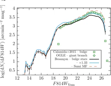
lo g( d N /d F 81 4W ) [a rc m in − 2 m ag − 1 ] F 814WVega Calamida+2015 – bulge OGLE – giant branch Besan¸con – bulge stars –×1.33 – Sumi MF 0.5 1 1.5 2 2.5 3 3.5 4 12 14 16 18 20 22 24 26
Figure 5. Comparison of Besanc¸on model star counts for the bulge population as a function of magnitude F 814WVega at
(`, b) = (1.◦35, −2.◦70) to those measured in the HST SWEEPS field at (`, b) = (1.◦25, −2.◦65), which lies close to the expected WFIRST fields. Green squares show bulge-only star counts from
HSTCalamida et al.(2015) and diamonds show counts of red
gi-ant branch stars in the same area from OGLE-III (Szyma´nski et al. 2011). The HST stars were selected to be bulge stars by proper mo-tion cuts, and have been corrected for the approximate efficiency of this cut. The solid black line shows the BGM1106 prediction, with error bars denoting the Poisson uncertainty of the catalogs. While there are differences in the detailed shape of the star count distri-bution, integrated over the range F 814W = 19–26.5, BGM1106 under-predicts the total number of stars by 33%; the blue line shows the BGM1106 scaled up by this factor. The dashed black line shows the BGM1106 model star counts if the mass function is changed in the bulge to match mass function 1 ofSumi et al.(2011), namely a broken power law with slopes of -1.3 and -2.0 (dN/dM ) each side of a break at 0.7M .
2008;Calamida et al. 2015) and now star counts (Calamida et al. 2015). By comparing star counts closer to the WFIRST fields we can hope to reduce the impact of any extrapolation errors when estimating an event rate correction.
Calamida et al.(2015) measured the magnitude distribu-tion of bulge stars by selecting stars with a proper modistribu-tion cut designed to exclude disk stars. Calamida et al.(2015) cor-rect for completeness using artificial star tests, but we add additional corrections for the efficiency of the proper motion cut (34 percent, A. Calamida, priv. comm.) and the field area (3.30 × 3.30), in order to plot the absolute stellar den-sity as a function of magnitude inFigure 5. We do not con-sider the bins at the extremes of the magnitude distribution which are likely affected by saturation or large incomplete-ness. To compare to the observed distribution, we computed the magnitude distribution of bulge stars in the BGM1106 sight line at(`, b) = (1.◦35,−2.◦70), which is the closest to the SWEEPS field.
BGM1106 matches the measured magnitude distribu-tion reasonably well between F 814WVega = 19.5 and 23,
though with minor differences in shape. BGM1106 starts to significantly underpredict the number of stars fainter than F 814WVega = 23. Brighter than F 814WVega = 22.9,
Calamida et al.(2015) find 10 percent more stars than the BGM1106 predicts. Integrated over the magnitude range F 814WVega = 19–26.5 BGM1106 under-predicts star counts by 33 percent. The magnitude of the discrepancy is very similar to that we found between the BGM1106 and the Holtzman et al. (1998) luminosity function, giving us some confidence that there is no significant gradient in the BGM1106’s star count discrepancy. We adopt the star count scaling factor offsc= 1.33.
The cause of the discrepancy between model and data can be partially explained by the BGM1106’s choice of ini-tial mass function (IMF) in the bulge, dN/dM ∝ M−1.0. Adopting a more reasonable mass function (e.g., mass func-tion number 1 from Sumi et al. 2011,dN/dM ∝ M−2.0 forM > 0.7M anddN/dM ∝ M−1.3for0.08 < M < 0.7M ), and assuming that the BGM1106 star counts were normalized using turn-off stars of1.0M , produces the lu-minosity function prediction shown by the dashed line in the plot. This mass function over-predicts the star counts fainter thanF 814WVega ≈ 20, but better matches the shape of the entire observed luminosity function between IVega ≈ 19– 26. Both the original and modified BGM1106 mass functions slightly under-predict the number of giant branch star counts from the same sight line detected by OGLE (Szyma´nski et al. 2011), which have not been corrected for incompleteness. We note here that we do not adopt an alternative mass func-tion (e.g, mass funcfunc-tion 1 fromSumi et al. 2011), but discuss the impact of the mass function on our results in section6.
3.2.2. Comparison to Microlensing Event Rates Since writingP13,Sumi et al.(2013) published measure-ments of the microlensing event rate towards the bulge, in addition to optical depth measurements. Measurements of the event rate per source star allow a more direct route to es-timating any corrections to the model’s predicted event rates, so here we only perform a comparison to the event rates and not the optical depths. For the comparison we use the event rates fromSumi & Penny(2016), which corrected theSumi et al.(2013) event rates and optical depths for a systematic error in estimates of the number of source stars monitored.
Sumi et al.(2013) present event rates for two samples of events, the “extended red clump” (ERC) sample composed of events with source stars brighter thanI = 17.5 and colors selected to only include the bulge giant branch, and the “all stars” (AS) sample composed of all events withI < 20 and no color cut. We selected star catalogs from the BGM1106 to match these samples, and computed event rates per source Γ by Monte Carlo integration over this source catalog and a lens catalog with no magnitude or color cuts (seeAwiphan
E ve n t R at e P er S ou rc e Γ [1 0 − 6 y r − 1 ] b [deg]
MOA All Star MOA Ext. RC Besan¸con ×2.11 0 10 20 30 40 50 60 70 -7 -6 -5 -4 -3 -2 -1 0 fΓ= 2.11± 0.29
Figure 6. Comparison of the microlensing event rate per source predicted by the Besanc¸on model to the (Sumi & Penny 2016) re-vision of measurements by (Sumi et al. 2013). Black data points show measurements for all source stars, while red data points show measurements for the extended red clump source stars (see text for details). The thin line shows the BGM1106’s prediction of extended red clump event rates, and the thick red line shows this prediction af-ter multiplication by the best fit scaling parameaf-ter fΓ= 2.11±0.29. et al. 2016, for a detailed description of such calculations). The small angle of the Galactic bar to the line of sight in the BGM1106 (∼12◦) results in the bulk of our AS sam-ple source stars lying in front of most of the bulge stars. This leads to significantly smaller event rates per source than would be expected for a more reasonable bar angle of ∼30◦(e.g.Wegg & Gerhard 2013;Cao et al. 2013), which could lead us to over-correcting the event rates. We therefore only compare to the ERC sample event rates.
Figure 6shows the predicted model event rates, averaged over the range −0.53 < ` ≤ +2.73, and the data from Sumi & Penny(2016), which was averaged over the range |`| < 5. BGM1106 predicts a lower event rate than is mea-sured. At latitudes|b| < 1.5 the predicted ERC event rate turns over likely because extinction begins to limit the range of distances over which significant numbers of bulge giants pass the ERC color and magnitude cuts; at more negative latitudes, where the observations we compare to were made, the extinction likely has a smaller impact. We find that mul-tiplying the BGM1106 event rates by a constant scaling fac-torfΓ = 2.11± 0.29 yields a good match to the observed ERC rates, with χ2 = 1.58 for 3 degrees of freedom. Al-though the model predictions cover a smaller range of` than the measurements,Sumi & Penny(2016) results binned by` indicate only a relatively weak dependence ofΓ on|`|.
3.2.3. Adopted Event Rate Scaling
InP13 we scaled the microlensing event rates computed using the BGM1106 by making the assumption that all of the relevant distributions (e.g., kinematics, mass, and
den-sity) were reasonable, but that there could be errors in the normalization of the numbers of source and lens stars. To make a correction for the number of source stars we directly compared the BGM1106 predictions to deep star counts mea-sured by HST. To estimate the correction for the number of lens stars, we compared model predictions to measurements of the microlensing optical depth. This has the advantage that, should the density distribution and mass function of stars in the model be reasonable, the necessary correction to the event rate due to lenses should scale with the optical depth discrepancy between model and data. However, as we have described in the preceding subsections and will expand on in Section 6, the density distribution (specifically the bar angle of the bulge), the bulge mass function, and the kinematics of bulge stars in the BGM1106 are inconsistent with current measurements. These will affect the event rate and optical depth in different ways that are not trivial to calculate. This makes any simple scaling of the event rate based on optical depth comparisons suspect. In contrast, a scaling based on measured event rates is far more direct with fewer assump-tions. Therefore, to correct the event rates predicted by the Galactic model, we adopt the event rate scaling factor
f1106,W F IRST = fscfΓ, (6) where
fsc= 1.33, andfΓ = 2.11, (7) for a total event rate correction of
f1106,W F IRST = 2.81, (8)
which is about20% larger than the scaling adopted inP13. We will discuss the impact of uncertainties and innaccura-cies in the Galactic model beyond the event rate scaling in Section 6.
We apply thef1106,W F IRST scaling throughout the paper as our fiducial event rate normalization. However, we will also present our main results with the scalings used for each of the WFIRST reports in order to aid comparison to these earlier works; these results using obsolete scalings are pre-sented inTable 5inSection 4. We note, however, that when applying the obsolete scaling, we did not include a factor of 1.475 in the scaling that was used in theGreen et al.(2012). This factor was used to account for a factor of 2.2 discrep-ancy in the microlensing detection efficiency of ourGULLS simulations and simulations performed by D. Bennett, based on Bennett & Rhie (2002) and updated for simulations of WFIRST (Green et al. 2011); 1.475 was the geometric mean of the relative detection efficiencies for planets of1M⊕with a period of2 years. The cause of the difference in detection efficiencies was not conclusively tracked down. However, at fixed period, the projected separations ∝ M−5/6, and the detection efficiency is a strong function ofs, so a difference
between the host mass function of the simulations (see Sec-tion 3.2.1andSection 6.2.3) is likely to cause a significant difference in the detection efficiency at fixed period. Aver-aged over a range of semimajor axis, as we have done in the simulations presented in Section 4, we can expect any dif-ference in the detection efficiency at fixed planet mass to be significantly smaller.
3.3. The WFIRST fields
For the IDRM, DRM1, DRM2, and AFTA simulations, the field placement was not rigorously optimized. We show the fields we adopted for each design inFigure 7. For IDRM, DRM1 and DRM2, the field placement is significantly differ-ent than what it would be in reality if each design were flown. This is due to uncertainties in the orientation of the detectors in the instrument bay. We therefore chose the simplest field orientation we could, aligning the principle axes of the fields with Galactic latitude and longitude. Note however, that this is an optimistic assumption, as the extinction and event rate at zeroth order depend strongly onb but weakly on `, so de-tector orientations that align the long axis with` are likely to be close to optimal. For the IDRM, DRM1 and DRM2 field layouts we accounted for gaps between detectors in the focal plan by placing the twice the sum of all chip gaps between each of the fields.
For AFTA we considered the field layout more carefully. The telescope instrument bay already exists, setting the ori-entation of the field and constraining the layout of detectors within it. Coincidently the orientation of the WFI focal plane for AFTA is within a couple of degrees of aligned with Galac-tic coordinates. From spring to fall seasons the orientation of the detector will be rotated by180◦, which means that with the curved geometry of the active focal plane, the fields ob-served will not be exactly the same. For the layout shown this results in∼90% of stars that fall on a chip in spring sea-sons also falling on a chip in the fall seasea-sons. Occasional gap filling dithers could be used to ensure some observations in both spring and fall for all events.
Between the AFTA design and Cycle 7, the WFIRST wide field instrument was redesigned and consequently the field orientation was rotated by90◦. Additionally, the spacecraft’s slew and settle time estimates were updated, and were more than twice that we had assumed for the AFTA design. These two changes led us to conduct an optimization of the field layouts. This optimization is described inSection 5.4. With this field layout we can expect to detect∼27, 000 microlens-ing events with|u0| < 1 and roughly twice this with |u0| < 3 during the course of the mission. While there are three times as many events with |u0| < 3 compared to |u0| < 1, the maximum magnification of a Paczynski (1986) single lens lightcurve at|u0| = 3 is only 1.017, compared to 1.34 at
b ( ◦ ) ℓ (◦) b ( ◦) AH -2 -1 0 1 2
IDRM
DRM1
-2 -1 0 1 2 -2 -1 0 1 2DRM2
-2 -1 0 1 2 0 0.5 1 1.5 2 2.5 3 3.5 4AFTA
AH b ( ◦) ℓ (◦) N1M⊕ deg−2 0 0.5 1 1.5 2 2.5 3 3.5 4 WFIRST Cycle 7 -2 -1 0 1 2 -2 -1 0 1 2 10 20 30 40 50 60 70 80 90 WFIRST Cycle 7Figure 7. Assumed field placement for each WFIRST design, plot-ted over a map of H-band extinction (Gonzalez et al. 2012). The gaps between IDRM, DRM1 and DRM2 fields were included to mimic the effects of gaps between detectors. For the AFTA and Cycle 7 simulations we accounted for the individual detector place-ment within each field more carefully, so fields are close-butted (note the curved focal plane). Note also that in reality the 1-m-class designs would also likely have curved detector layouts and that, unlike the AFTA and Cycle 7 designs, the fields would proba-bly not be orientated with their principle axes aligned with Galactic coordinates. The black diamond in the top panels shows the lo-cation of the HST SWEEPS field. In the Cycle 7 panel, colored dots show the detection rate of 1M⊕planets per square degree as
a function of position for the Cycle 7 design. A version of the Cycle 7 plot is available athttps://github.com/mtpenny/
wfirst-ml-figures.
|u0| = 1, so only on brighter stars will it be possible for WFIRSTto detect these low-magnification events.