HAL Id: hal-00295455
https://hal.archives-ouvertes.fr/hal-00295455
Submitted on 28 Jun 2004
HAL is a multi-disciplinary open access
archive for the deposit and dissemination of
sci-entific research documents, whether they are
pub-lished or not. The documents may come from
teaching and research institutions in France or
abroad, or from public or private research centers.
L’archive ouverte pluridisciplinaire HAL, est
destinée au dépôt et à la diffusion de documents
scientifiques de niveau recherche, publiés ou non,
émanant des établissements d’enseignement et de
recherche français ou étrangers, des laboratoires
publics ou privés.
Meteoroid velocity distribution derived from head echo
data collected at Arecibo during regular world day
observations
M. P. Sulzer
To cite this version:
M. P. Sulzer. Meteoroid velocity distribution derived from head echo data collected at Arecibo during
regular world day observations. Atmospheric Chemistry and Physics, European Geosciences Union,
2004, 4 (4), pp.947-954. �hal-00295455�
www.atmos-chem-phys.org/acp/4/947/
SRef-ID: 1680-7324/acp/2004-4-947
Chemistry
and Physics
Meteoroid velocity distribution derived from head echo data
collected at Arecibo during regular world day observations
M. P. Sulzer
Arecibo Observatory, Arecibo, Puerto Rico
Received: 1 October 2003 – Published in Atmos. Chem. Phys. Discuss.: 4 February 2004 Revised: 17 June 2004 – Accepted: 17 June 2004 – Published: 28 June 2004
Abstract. We report the observation and analysis of ion-ization flashes associated with the decay of meteoroids (so-called head echos) detected by the Arecibo 430 MHz radar during regular ionospheric observations in the spring and au-tumn equinoxes. These two periods allow pointing well-above and nearly-into the ecliptic plane at dawn when the event rate maximizes. The observation of many thousands of events allows a statistical interpretation of the results, which show that there is a strong tendency for the observed mete-oroids to come from the apex as has been previously reported (Chau and Woodman, 2004). The velocity distributions agree with Janches et al. (2003a) when they are directly compara-ble, but the azimuth scan used in these observations allows a new perspective. We have constructed a simple statistical model which takes meteor velocities as input and gives radar line of sight velocities as output. The intent is to explain the fastest part of the velocity distribution. Since the speeds interpreted from the measurements are distributed fairly nar-rowly about nearly 60 km s−1, double the speed of the earth in its orbit, is consistent with the interpretation that many of the meteoroids seen by the Arecibo radar are moving in or-bits about the sun with similar parameters as the earth, but in the retrograde direction. However, it is the directional infor-mation obtained from the beam-swinging radar experiment and the speed that together provide the evidence for this in-terpretation. Some aspects of the measured velocity distribu-tions suggest that this is not a complete description even for the fast part of the distribution, and it certainly says nothing about the slow part first described in Janches et al. (2003a). Furthermore, we cannot conclude anything about the entire dust population since there are probably selection effects that restrict the observations to a subset of the population.
Correspondence to: M. P. Sulzer
1 Introduction
The Arecibo 430 MHz radar is a very powerful and sensitive instrument used primarily for measurements of incoherent scatter (IS) in the earth’s ionosphere. In the last several years it has been used for the observation of small meteoroids as they penetrate into the atmosphere, depositing sufficient en-ergy to cause detectable ionization in the immediate region of the decaying meteoroid resulting from collisions with at-mospheric particles. The result is the so-called head echo, which is not yet well understood. The Arecibo instrument is one of several high-sensitivity radars providing these mea-surements (see the list of references in Chau and Woodman, 2004). Most of these observations have used observational techniques designed especially for observation of the very brief flashes of ionization associated with the collisions. It is possible to use much data intended for ionospheric observa-tions to detect the decay of the meteoroids and measure some of the associated parameters, such as the time of the flash, its intensity, its altitude, and the velocity component along the radar line of sight. However, it is necessary to have access to the raw voltage samples, not the analyzed data. We used a high resolution mode intended for measuring the IS spec-trum in the E region of the ionosphere. The spectral width of the IS ion line is much less than the Doppler shifts of most of the head echos, and so in this case the wide bandwidth used to obtain good range resolution allows observation of the head echos, which have very narrow spectra located at large Doppler shifts. Most current IS measurements made at Arecibo sample the necessary bandwidth even if the res-olution is not necessary, and so most of the data are at least potentially suitable for analysis of meteor head echos. How-ever, the coded long pulse technique used for observations described here is particularly well-suited because the appro-priate analysis makes it very easy to locate the meteoroid path in height and frequency.
948 M. P. Sulzer: Arecibo world day meteor velocities
Viewed from
North Summer Solstice
Autumn
Equinox SpringEquinox Apex
Winter Soltice Pole is tilted towards the apex, lowering the zenith of the AO radar 4.7° below the ecliptic.
Pole is tilted away from the apex,raising the zenith of the AO radar23 + 18.3° above the ecliptic.
Fig. 1. The location of the radar with respect to the ecliptic plane as a function of the season.
We present results from two periods, the spring and au-tumn equinoxes. The Arecibo radar cannot point more than 20◦from the zenith, and sensitivity issues restrict the point-ing in these ionospheric observations to 15◦. As meteor ob-servations have previously, we augment this range by using the seasonal changes of the location of the radar with respect to the ecliptic plane. Figure 1 shows that in the spring the radar zenith is well above the ecliptic at dawn, while in the fall it lies almost in it, and so points nearly along the apex as the meteor event rate maximizes. These differences in point-ing have important consequences for the observations.
We have a sufficiently large number of events so that we can make conclusions requiring statistical analysis, and we see the previously-reported tendency for the apparent source of the meteoroids to lie along the apex defined by the mo-tion of the earth around the sun (Chau and Woodman, 2004). The speeds computed from our measurements are distributed fairly narrowly just under 60 km s−1. Since this is nearly double the speed of the earth in its orbit, the obvious interpre-tation, given the directional information, is that most of the meteoroids seen by the Arecibo radar are moving in orbits about the sun with similar parameters as the earth, but in the retrograde direction. We do not even claim this as a potential description for the complete population, since we currently have no way to remove certain observational biases, and it is not clear how much information would be available from a much larger set of data after the application of careful mod-eling. A weaker distribution of slower particles is seen in the fall observations, and possibly in the spring observations. This was first reported by Janches et al. (2003a).
S (180) S (540) N (360) Time Az im ut h An gl e E W Repetition Period x Repetition Period 2x
Fig. 2. This drawing shows that the repetiton period of a target located in the north (or south) is twice as high as a target located in the east (or west).
We have constructed a simple statistical model intended to show that the above interpretation is consistent with the general properties of the fastest part of the observed velocity distribution. It is not an accurate model intended for param-eter fitting, but is only a first step in this direction. This in-terpretation helps explain why meteors seem to come “down the beam” at Arecibo. This question is discussed in Janches et al. (2003a) and Janches et al. (2003b), which favor an in-terpretation based on atmospheric effects. Our inin-terpretation does not exclude atmospheric effects; in fact, we have had to assume such an effect to make it work.
2 Experiment Description
The ionospheric experiment that provided the data for the meteor observations we describe here is one mode of Arecibo’s World Day observations. The pointing angle from the zenith (zenith angle, or αza) is fixed at 15◦, while the azimuth angle (αaz), measured from north in the eastward direction, is varied. Ideally, the azimuth angle would con-tinue to increase at the maximum (slew) rate, but in practice it is necessary to stop and turn around so that cables carry-ing power and information do not break. The procedure is to scan from 180◦(looking south with the line feed) to 540◦, a complete revolution. Then the motion stops, and the pointing returns to 180◦. It is necessary to account for the time spent motionless at the limits of the motion and accelerating near the limits in some of the data analysis described later.
Figure 2 shows an important consequence of the pattern of azimuth motion. A target located in the north or south would be sampled uniformly with an interval of 180◦(about 8 min). However, a target located in the east or west has a funda-mental period of about 16 min, but the time series would also
Ecliptic plane Equator Apex Arecibo Observatory N is 0° azimuth Azimuth is measured in this direction. vz vx vy αza = 15° αx = 41.3° meteor velocity Sun vz' vls 23° 18.3°
Fig. 3. Observations during the Spring Equinox at dawn. The radar and the apex define a plane perpendicular to the ecliptic.
have additional periods resulting from the alternating short and long intervals between samples. The time series of a pa-rameter associated with a target such as line of sight velocity shows this effect also.
Figure 3 shows in detail the spring conditions correspond-ing to the rightmost part of Fig. 1. At dawn when the pro-jection of the radar zenith in the ecliptic plane points into the apex, the zenith pointing position is 41.3◦north of the eclip-tic.
It is convenient to express the meteor velocities in a coor-dinate system where the z-axis points to the apex, where the x-axis points in the eastward direction in the ecliptic plane, and where the y-axis points northward perpendicular to the ecliptic plane. It is also convenient to find the radar line-of-sight velocities as a function of the x, y, and z components. The first step in this process is to define a x0y0z0 system by rotating about the x-axis so that the z0 axis is parallel to the radar zenith. The velocity transformation is
vx0 vy0 v0z = 1 0 0 0 cos αx−sin αx 0 sin αx cos αx vx vy vz , (1)
where αxis defined in Fig. 3
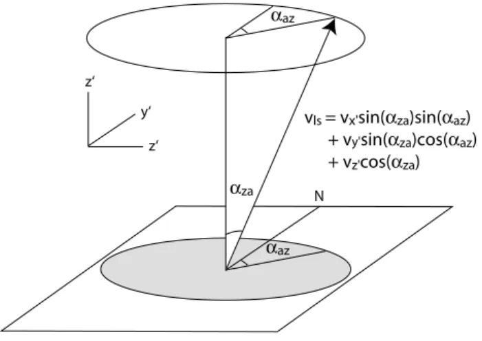
Figure 4 shows the transformation to the line-of-sight ve-locity vls. The transformation is
vls =vx0 sin αzasin αaz (2)
+vy0 sin αzacos αaz+v0zcos αza.
The flat plane in Fig. 4 would be tangent to the sphere of Fig. 3 at the location of the Arecibo Observatory.
At times other than dawn, the radar no longer lies in the yzplane, and since the angle between the equator and eclip-tic changes, αxis a function of time. Also there is a rotation
vls= vx'sin(αza)sin(αaz) + vy'sin(αza)cos(αaz) + vz'cos(αza) z‘ y‘ z‘ N αaz αaz αza
Fig. 4. Computing the radar line of sight velocity from a velocity
vector v0.
about the y axis. We do not need to consider this more gen-eral transformation in detail.
The observations used a radar pulse 400 µs in length; the pulse modulation was binary phase using a pseudo-random phase sequence with a baud length of 2 µs, and the trans-mission used a different code for each pulse. Sulzer (1986) describes the application of this technique to IS. In that ap-plication the signal has a correlation time that is shorter than the pulse length, and the technique allows the measurement of the signal autocorrelation function with range resolution equal to the baud length of the code. However, the correla-tion time is much longer than the inverse of the baud length (narrow spectrum), and it is possible to speed up the calcula-tions for the IS spectrum while losing the possibility of mea-suring the meteor parameters by failing to calculate the full bandwidth. Thus it is necessary to perform an independent analysis for the meteors. This analysis takes longer than real time, but it is nonetheless convenient because the raw volt-age samples are stored on disk for some time after the exper-iment.
The spring experiment used the line feed only, while the fall used both the line feed and Gregorian. The presentation here includes only the linefeed data, since the analysis of the Gregorian data is not complete.
The inter-pulse period of this experiment is 10 µs; this is longer than one would like for a detailed analysis of the head echo, but perfectly satisfactory for counting powers, heights, and frequencies. Meteors are occasionally seen for as long as five inter-pulse periods, but often are visible for only one. There are two possible ways to analyze the raw data. The first is the standard coded long pulse analysis in which one multiplies the code into the data samples beginning at some point, which defines the decoded range. One computes the power spectrum of the product, and does this for each
950 M. P. Sulzer: Arecibo world day meteor velocities 3 3.5 4 4.5 5 5.5 6 6.5 7 0 -10 -20 -30 -40 -50 -60 -70 -80 Time (AST) Ve lo cit y (k m /s ec ) S S
Fig. 5. The velocities of all meteoroids on 20 March 2003 from 03:00 to 07:00 AST. 0 20 40 60 80 -3.5 -3 -2.5 -2 -1.5 -1 -0.5 0 Frequency (hr-1) Lo g1 0 of R el at ive C ou nt N um be r
Fig. 6. The power spectrum of the function formed by binning the detections by azimuth. The result is the average of the four days, 20–23 March 2003, covering the time period 4.6 to 6.1 AST.
possible range. The other method is to decode the time se-quence as one would for a power profile, but to repeat the decoding on frequency shifted versions of the signal. It turns out that the two methods treat a single meteor signal in nearly identical ways, but the processing of the overlapping of mul-tiple signals is different. However, even two meteors at once is a rare event, and the ionospheric clutter cannot be decoded in any case since its correlation time is too short. The first analysis is a simple modification of the standard ionospheric analysis, making sure that the high Doppler shifts are not dis-carded in order to speed up the computations, and it guaran-tees that the ionospheric clutter is randomized, the best avail-able option if it cannot be eliminated. Thus we chose the first method.
The analysis is divided into two steps, and the results of the first step are saved since it is convenient to redo the second in different ways as required. The first step computes the spec-tra for all ranges for the samples from a single radar pulse. It is not possible to save these spectra, since they require more storage space than the original samples, but since we expect either no detection or the detection of a single meteor, we find the maximum power in any of the spectra and save its range, frequency, and intensity as well as time and pointing information. We do this for the received power from each radar pulse.
The second step is to find which of the saved maxima are meteor detections and which are noise. This involves find-ing a threshold in which the majority of the events define a baseline from which the few deviate. We use a sliding time interval since the noise level is a function of time. The analy-sis would have been easier if we saved an average noise level for reach radar pulse in the first step, but this would make lit-tle difference in the results during the night and around dawn, the time period used in this paper.
3 Spring Observations
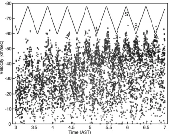
The spring observations occurred on four days near the spring equinox of 2003. We concentrate on the four dawn pe-riods since the meteor count is maximum at this time. Figure 5 shows the velocities versus time of all detected events from 03:00 to 07:00 AST on 20 March 2003. Each event is a small dot; the solid line indicates the azimuth positions. Note that near dawn there is a periodic ripple in the maximum veloc-ity which is locked in phase to the azimuth motion, and that the maximum velocity occurs when the azimuth is pointed to the south. When the radar points south, its projection along the apex is at its maximum, and so Fig. 5 is consistent with velocities aligned along the apex, at least approximately.
Several hours before dawn the ripples have half the fre-quency. This is because an apex-aligned feature has a sig-nificant east-west component before dawn. As explained in Sect. 2 east-west features have twice the period, or half the frequency of north-south features. Obviously the ripple is complicated, and we will not try to determine its exact shape. This tentative conclusion of alignment with the apex would be doubtful if there were some selection effect, per-haps instrumental, which emphasized different parts of the population as a function of azimuth angle. Such a bias would likely be revealed by the event count rate as a function of azimuth angle. Figure 6 shows a power spectrum of the se-ries obtained by by finding the event counts in 128 uniformly spaced azimuth bins. The plot shows the sum of the results from four dawn periods from 4.6 to 6.1 AST. The dates are the 20–23 March 2003. The result is almost what one would expect from random variations only in the count rate. The zero frequency peak indicates the total count rate, and there is only one other peak that might be significant, and it does
200 300 400 500 0 -10 -20 -30 -40 -50 -60 -70 -80 4.81818 9.63636 14.4545 19.2727 24.0909 28.9091 33.7273 38.5455 43.3636 48.1818 Li ne o f S ig ht V el oc ity
Azimuth Angle (180° and 540° South, 360° North)
Nu m be r o f C ou nts South W N E South
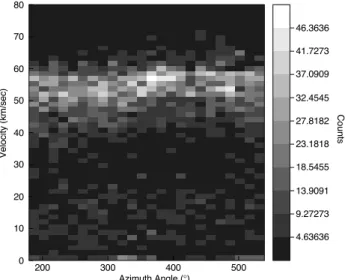
Fig. 7. The distribution of the velocities with azimuth angle from four days of spring equinox data (20–23 March 2003).
not lie at a harmonic of the rotation time. We conclude that there are no significant biases which would show up in an analysis of the count rates.
Figure 7 shows the results of putting the line-of-sight ve-locities from 20–23 March 2003 into 24 azimuth bins. The maximum is not centered exactly in the southern direction as one might (mistakenly) expect from Fig. 5. This effect is significant since it is visible in the individual days after az-imuth binning. The depth of the minimum in approximately the northern direction provides a method to see if the center of the velocity distribution lies in the ecliptic plane, as we can show using the analysis of Sect. 2.
Figure 8 shows two cuts in the velocity direction from Fig. 7. The dark thin line is from the maximum (nearly south); it has a high peak in the distribution. The thicker gray line is from 180◦away; it is less highly peaked. This indicates that there is dispersion in the velocity component in the y direction (perpendicular to the ecliptic).
To further demonstrate the plausibility of the interpreta-tion involving alignment with the apex, we have computed an approximate statistical model using the transformation be-tween the meteor velocity and the line of sight velocity of Sect. 2. In the model we assume that meteoroids initially have a speed of 60 km s−1, that they have some average and
random (Gaussian distributed) x and y velocities, and that the speed decreases by a random amount (χ -square distribu-tion with one degree of freedom) before observadistribu-tion. The reason for the last assumption is discussed below. The χ -square distribution with one degree of freedom just means that the speed decrements are found by generating Gaussian random numbers, squaring, and multiplying by a scale factor. For the fall case we have assumed values of −5 km s−1 for the systematic x and y components. These are just
approxi-0 10 20 30 40 0 5 10 15 20 25 30 35 40 45
Line of Sight Velocity
Nu m be r o f C ou nt s
Fig. 8. Constant azimuth cuts at the maximum and minimum from the results of the previous figure.
200 300 400 500 0 -10 -20 -30 -40 -50 -60 -70 -80 3.81818 7.63636 11.4545 15.2727 19.0909 22.9091 26.7273 30.5455 34.3636 38.1818 Azimuth Angle (°) Ve lo cit y (k m /s ec ) Co un ts
Fig. 9. A primitive model of the results shown in Fig. 7.
mate values; however, neither could be zero for the model to work. They imply that the center of the distribution is 5◦east and north of the apex. We have also assumed 8 km s−1for the sigmas of the Gaussian distributions, giving roughly 8◦ of dispersion in the direction perpendicular to the apex. We have low sensitivity at dawn in the x direction, and so that value could vary a lot. It is the y value that determines how flat the distribution is in the south, and so it matters. Finally we have assumed that the scale factor in the speed decrement is 5 km s−1.
As we shall see below, and as Janches et al. (2003a) has shown, there is a separate distribution of apparently slow par-ticles, and we are not attempting to model this, or the medium speeds.
952 M. P. Sulzer: Arecibo world day meteor velocities Arecibo Observatory Ecliptic plane meteor velocity N is 0° azimuth Azimuth is measured in this direction. Apex Equator αza = 15° αx = 4.7° vz vx vy Sun
Fig. 10. Observations at the autumn Equinox.
Figure 9 shows the model; although it is not perfect it does a pretty good job of reproducing the measurements near the sinusoid. It is interesting to compare this model with the one required for the fall results.
4 Fall Observations
The autumn equinox provides an opportunity to verify some of the tentative conclusions made in the last section. Fig-ure 10 shows the relationship between the radar pointing and the apex. Note that the radar zenith points nearly along the apex at dawn, and so the azimuth track holds nearly a con-stant 15◦angle with respect to the apex. This means that the higher frequency temporal variations seen at dawn should be very small, while structure should still be seen away from dawn, if there is alignment with the apex.
Figure 11 shows the velocity data for 24 September 2003 in the same format as Fig. 5 did for the March data. The ripples at dawn are indeed missing, and structure is visible before dawn. It has the expected low frequency component, and the paired features seen in Fig. 2 are also visible, marked by vertical arrows. Of course this apex-aligned structure in the velocity lies between north and east, and so the spacing in the close features is wider than shown in Fig. 2 for the east-west structure. (One can think of sliding the beads down the lines until the right angle is reached.)
Figure 12 shows the distribution of the velocities with azimuth angle from four days of fall equinox data (23–26 September 2003), about 8 000 total events, or roughly 4 000 meteors. (The average number of radar pulses seeing a sin-gle meteor is two.) It is equivalent to Fig. 7 for the spring; it resembles that figure in that the velocities are concentrated near −60 km s−1, but the systematic variation with azimuth
3 3.5 4 4.5 5 5.5 6 6.5 7 0 10 20 30 40 50 60 70 80 Time (AST) Ve lo cit y (k m /s ec )
Fig. 11. The velocities of all meteoroids on 24 September 2003 from 03:00 to 07:00 AST.
is small in this case as expected. We have removed some interference from the data from 23 September 2003 only.
Figure 13 shows the same data as Fig. 12 summed over azimuth angle. This distribution is essentially the same as Fig. 4 of Janches et al. (2003a) for the dawn time period look-ing south with the Gregorian feed. The radar pointlook-ing direc-tion associated with the data of that figure is as close as pos-sible to the pointing direction of the fall data described here. Thus the two data sets are consistent. However, it should be noted that we have not verified that all the the events are me-teors, and so the the counts at the highest speeds (above the peak) might be false. Janches et al. (2003a) does not show such meteors.
Figure 14 shows a model of the fall observations. The parameters are not identical to the spring model; the average xand y component have been set to zero. These observations are very sensitive to an average y component; the value used for the spring observations is many times too large. That is, these velocities come from right from the apex at least with respect to the y direction. The dispersions in all directions have changed from the spring model.
5 Disussion and Conclusions
We believe that the data and model of the two previous sec-tions are a strong corroboration of the results of Chau and Woodman (2004), which first described the apex alignment. Some discussion is necessary, however. First, there is the matter of the slightly different directions in the spring and fall. It is not a contradiction that the directions measured are in the two seasons differ by a small amount. In the fall, the radar is located nearly in the ecliptic plane, while in the spring, it is located well above it. This is a large enough
200 300 400 500 0 10 20 30 40 50 60 70 80 4.63636 9.27273 13.9091 18.5455 23.1818 27.8182 32.4545 37.0909 41.7273 46.3636 Azimuth Angle (°) Ve lo cit y (k m /s ec ) Co un ts
Fig. 12. The distribution of the velocities with azimuth angle from four days of fall equinox data (23–26 September 2003).
0 10 20 30 40 50 60 70 80 0 100 200 300 400 500 600 700
Fig. 13. The distribution of the velocities summed over azimuth angle from four days of fall equinox data (23–26 September 2003).
difference so that there could be some differences in the par-ticle orbits that the radar sees. It is the physical position of the radar above the ecliptic that matters. We do not expect the distribution of meteors to appear any different as the pointing direction of the radar is changed with azimuth motion since the observations are only about 100 km from the surface of the earth, and so the horizontal distance from two pointing positions separated by 180◦is only about 50 km.
If we make the reasonable assumption, based on the di-rectional information measured in both the spring and the fall, that the particles are in retrograde orbits with nearly the same parameters as the orbit of the earth, then the total ve-locity must be 60 km s−1, twice the speed of the earth in its orbit. We need to explain why we assumed an average loss of
200 300 400 500 0 -10 -20 -30 -40 -50 -60 -70 -80 5.18182 10.3636 15.5455 20.7273 25.9091 31.0909 36.2727 41.4545 46.6364 51.8182 Azimuth Angle (°) Ve lo cit y (k m /s ec ) Co un ts
Fig. 14. A primitive model of the results shown in Fig. 12.
several km s−1before observation. During the radar-visible phase of the entry of a particle, it slows by several km s−1; this can be verified from this data set or others. On average, we see a particle when it is partly through its radar-visible path, because most do not come right through the center of the beam. This means that we see particles when they have slowed, and several km s−1 is a reasonable number for the average lost speed. This provides the source of the down-ward dispersion in the magnitude of the velocity, and allows the assumption that the speeds are all very nearly the same before they enter the atmosphere.
We have explained the “down the beam” effect described in, for example, Janches et al. (2003a) and Janches et al. (2003b), as primarily a geometric effect. If one observes at dawn, and the meteors tend to come from the apex, then they will be seen to come “down the beam”. If one does not know about the possibility of apex alignment and assumes that the source direction is random, then an atmospheric effect would appear to be the probable complete explanation for the align-ment with the beam. Of course, we have had to assume an atmospheric effect in order to make the geometrical model work. Thus we are not saying that there are no atmospheric effects contributing to beam alignment. Indeed, all such ef-fects will need to be included in a complete model of the process and probably will be very important.
We have made very little use of the data except in the dawn periods. Data from all seasons and all times should be used simultaneously to make a single model. This would probably involve some modern inverse technique, and it would be a lot of work. However, it would probably be the only way to include selection effects, and thus allow the possibility of examining the properties of the full population.
954 M. P. Sulzer: Arecibo world day meteor velocities
Acknowledgements. The author thanks Diego Janches and Michael Nolan for essential discussions, as well as the organizers of and participants in the Radar Meteor Workshop held at Arecibo in March, 2003.
Edited by: J. Plane
References
Chau, J. L. and Woodman, R. F.: Observations of meteor-head echoes using the Jicamarca VHF radar in interferometer mode, Atmos. Chem. Phys., 4, 511–521, 2004.
Janches, D., Nolan, M. C., Meisel, D. D., Mathews, J. D., Zhou, Q. H., and Moser, D. E.: On the geocentric micrometer velocity distribution, J. Geophys. Res., 108, 1222–1235, 2003.
Janches, D., Nolan, M. C., and Sulzer, M. P.: Radiant measurement accuracy of micrometers detected by the Arecibo 430 MHz dual-beam radar, Atmos. Chem. Phys., 4, 621–626, 2004.
Sulzer, M. P.: A radar technique for high range resolution incoher-ent scatter autocorrelation function measuremincoher-ents utilizing the full average power of klystsron radars, Radio Science, 21, 1033– 1040, 1986.