Preliminary assessment of rockslide and rockfall hazards using a DEM (Oppstadhornet, Norway)

(1)

HAL Id: hal-00299171

https://hal.archives-ouvertes.fr/hal-00299171

Submitted on 18 Mar 2005

HAL is a multi-disciplinary open access

archive for the deposit and dissemination of

sci-entific research documents, whether they are

pub-lished or not. The documents may come from

teaching and research institutions in France or

abroad, or from public or private research centers.

L’archive ouverte pluridisciplinaire HAL, est

destinée au dépôt et à la diffusion de documents

scientifiques de niveau recherche, publiés ou non,

émanant des établissements d’enseignement et de

recherche français ou étrangers, des laboratoires

publics ou privés.

Preliminary assessment of rockslide and rockfall hazards

using a DEM (Oppstadhornet, Norway)

M.-H. Derron, M. Jaboyedoff, L. H. Blikra

To cite this version:

M.-H. Derron, M. Jaboyedoff, L. H. Blikra. Preliminary assessment of rockslide and rockfall hazards

using a DEM (Oppstadhornet, Norway). Natural Hazards and Earth System Science, Copernicus

Publications on behalf of the European Geosciences Union, 2005, 5 (2), pp.285-292. �hal-00299171�

(2)

International Center for Geohazards, Geological Survey of Norway, Leiv Eirikssons vei 39, 7491 Trondheim, Norway

2_{Quanterra, Tour-Grise 28, 1007 Lausanne, and Institut de G´eomatique et d’Analyse des Risques, University of Lausanne,}

Switzerland

Received: 17 November 2004 – Revised: 10 March 2005 – Accepted: 11 March 2005 – Published: 18 March 2005 Part of Special Issue “Landslides and debris flows: analysis, monitoring, modeling and hazard”

Abstract. The increasing availability and precision of digital

elevation model (DEM) helps in the assessment of landslide prone areas where only few data are available. This approach is performed in 6 main steps which include: DEM creation; identification of geomorphologic features; determination of the main sets of discontinuities; mapping of the most likely dangerous structures; preliminary rock-fall assessment; esti-mation of the large instabilities volumes.

The method is applied to two the cases studies in the Opp-stadhornet mountain (730 m alt): (1) a 10 millions m3 slow-moving rockslide and (2) a potential high-energy rock falling prone area. The orientations of the foliation and of the ma-jor discontinuities have been determined directly from the DEM. These results are in very good agreement with field measurements. Spatial arrangements of discontinuities and foliation with the topography revealed hazardous structures. Maps of potential occurrence of these hazardous structures show highly probable sliding areas at the foot of the main landslide and potential rock falls in the eastern part of the mountain.

1 Introduction

Very few data are often available at the beginning of the in-vestigation of a potential landsliding area. Nevertheless a preliminary assessment can be achieved using only a digi-tal elevation model (DEM) (Soeters and van Westen, 1996; Guzzetti et al., 1999; Van Westen, 2004). DEMs can usually be quite easily obtained from national topographic surveys, built with remote sensing methods (such as stereo airphotos or lidar) or by digitizing the contour lines of a topographic map (Van Westen, 2004).

The relief modeled by a DEM is the result of the interac-tions between numerous processes: erosion, deposition, tec-tonics, weathering, human activities, climate and vegetation.

Correspondence to: M.-H. Derron

(marc.derron@ngu.no)

Part of the information ”recorded” by a topographical sur-face is directly related to the stability of the slope and a mor-phological analysis of a DEM can reveal landsliding areas (McKean and Roering, 2004). We present here a procedure to extract as much as possible of this slope stability-related information by using only a minimal set of initial data (i.e. stereo airphotos and a topographical map).

Ideally this preliminary assessment should propose provi-sional answers to the following questions:

Where? – Location and geometry of the sliding mass. Which mechanism? – Sliding on a plane, wedge failures, toppling. . .

How big? – Volume, energy, propagation. . .

Structural and stability analysis with a DEM is made pos-sible by the recent development of geologically oriented GIS tools (G¨unther, 2003; Jaboyedoff, 2002, 2003).

The Oppstadhornet landslide area has been used as a “blind test” site for this preliminary assessment. The re-sults of this assessment have been compared to the rere-sults of field investigations (Blikra et al., 2001, 2002; Robinson et al., 1997).

2 Oppstadhornet landslide settings

The Oppstadhornet landslide is an unstable mountainside along the southern slope of the Oterøya island (Fig. 1), on the western coast of Norway (Blikra et al., 2001, 2002; Robin-son et al., 1997). The entire slope of Oppstadhornet shows multiple imbricated instabilities, from small rock falls to a large rockslide of several millions m3(a translational land-slide according to Cruden and Varnes, 1996). The area in-cludes granitoid gneiss that hosts two zones of schist, and subordinate meta-gabbros. All rocks are well foliated, typi-cally with a steep to moderate southward dip, i.e. towards the fjord.

Open crevasses and clefts reflecting block sliding are found within a kilometer wide and 700 m high area (Fig. 2). The slope of the soil-covered mountainside varies from 20–

(3)

286 M.-H. Derron et al.: Preliminary assessment of rockslide and rockfall hazards using a DEM

Fig. 1. (a) Relief map of Norway; (b) location of the Oppsatdhornet

site on the Oterøya island.

Fig. 2. Top fault scarp of the Oppsatdhornet landslide. The scarp is

about 600 m long, 50 m wide and 20 m high (location in Fig. 4).

30◦in the lower part to bare and steep cliff-faces in the upper and especially eastern part. Talus and block fields lay at the toe of the steeper portion. Further down, the area is vegetated with a dense forest.

A 2-D mechanical modeling indicates that part of the Opp-stadhornet slope can be involved in a large landslide due to the degradation of the material filling the joints or to a seis-mic dynaseis-mic loading (Bhasin and Kaynia, 2004).

Fig. 3. Illustration of the steps of the proposed approach.

3 Methods

For this preliminary assessment, we have used a procedure in 6 steps (Fig. 3). If a DEM is already available the step 0 can be avoided.

0. Building a DEM from a pair of stereo airphotos, 1. mapping the geomorphologic features relevant to slope

stability,

2. determination of the orientations of discontinuities, 3. kinematic feasibility tests and maps of distribution of

hazardous structural arrangements,

4. blocks propagation, shear/normal stress ratio on sliding planes,

5. estimation of volumes and of a shear stress-index using the sloping local base level.

3.1 Step 0: DEM extraction

A pair of black and white stereo airphotos and a regular pho-togrammetric processing have been used to build a 5 m reso-lution DEM. The nominal scale of the airphotos was 1:15 000 and the ground control points were collected using the local 1:50 000 topographical maps. The DEM and the orthophotos (Fig. 4) were processed with PCI-Orthoengine. This pho-togrammetric step could have been avoided if another DEM was available.

3.2 Step 1: DEM and orthophotos interpretation

The stereo airphotos and a 3-D model (the orthophotos draped on the DEM) from the step 0 were interpreted to ex-tract the geomorphologic features relevant to slope stability. This is a classical step to start the investigation of a landslide area by using either an analogical stereoscope or some digital stereoscopy softwares.

(4)

“slope aspect”, respectively). We used two methods to mea-sure the orientations of planar discontinuities on the DEM: a) the direct estimation of the slope of fault scarps (dip and dip direction), b) the calculation of the orientation of a plane defined by at least three points on a fault trace.

3.4 Step 3: Kinematic feasibility tests

This step provides the zones where sliding of rock masses can occur along discontinuities. The kinematic conditions that have to be satisfied to allow a planar sliding or a wedge failure are described in Hoek and Bray (1984), Norrish and Wyllie (1996) and Gokceoglu et al. (2000).

For a planar sliding, the three kinematics conditions are: 1) the strike of the potential sliding plane is close to the strike of the topographical slope (±20◦); 2) the dip of the sliding plane is less than the dip of the topographical slope; 3) the dip of the sliding plane is more than the angle of internal friction. At this stage of the investigation, no data about the angle of internal friction is available. So we used a simplified kinematic test for a planar sliding by using only the two first conditions. This test was performed with Matterrocking 2.0 (Jaboyedoff, 2002). This software identifies the cells of the DEM where the discontinuity makes an angle smaller than 90◦with the perpendicular to the topographic facet.

A similar approach has been used for the wedge failure hazard, considering that two discontinuities define a wedge. Again three geometric conditions should be satisfied to al-low a wedge failure: 1) the trend of the wedge axis is close to the dip direction of the topographical slope, 2) the plunge of the wedge axis is less than the dip of the topographical slope, 3) the plunge of the wedge axis is more than the angle of internal friction. Matterrocking 2.0 has been used to com-plete this test (Jaboyedoff, 2002). Assuming a continuous network of infinite discontinuities, the two sets of disconti-nuities make a network of wedges. The density of wedges in each cell of the DEM depends on: the average spacing of each set of discontinuities, the angle between the two sets, and the angle between the wedge axis and the topography (Jaboyedoff et al., 1996). The two angles are known, but not the average spacings. So we used arbitrary values (10 m) for the spacings. We get then a pseudo-number of wedge axis cutting each cell of the DEM. This number is interpreted as an indicator, presented here in quartiles, of the probability to satisfy the conditions for a wedge failure.

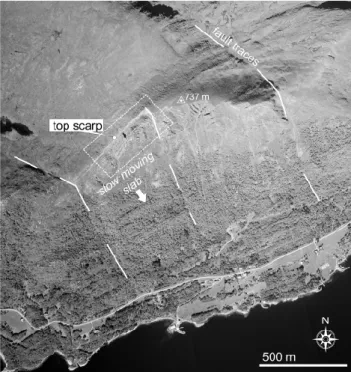
Fig. 4. Orthophoto of the Oppsatdhornet area (summit at 737 m),

with the scarp and the fault traces limiting the main landslide (rect-angle: area represented in Fig. 2).

3.5 Step 4: Rock fall assessment and rock mass stability Having identified and mapped two hazardous instability pro-cesses in the previous step, two indicators can be now calcu-lated without any new data:

1. The maximal velocities of falling blocks using a cone method model (ConeFall, Jaboyedoff, 2003). By as-suming the analogy of block fall with sliding, the cone method provides an estimate of the maximal transla-tional velocities of the blocks. The total kinetic en-ergy is divided into a rotational component (10%) and a translational component (90%). The critical angle (32◦) was estimated using the average slope of the screes. The presence of forested areas has not been taken into ac-count and the model tends to overestimate the veloci-ties (Jaboyedoff, 2003). Nevertheless, even if the final velocities are overestimated, they provide an important piece of information at this early stage of an investiga-tion.

2. Following G¨unther (2003), the ratio of the normal stress to the shear stress on a plane of discontinuity provides an indicator of stability. This approach is based on the estimation of the ratio shear/normal stress produced by the weight of rock at the vertical of a point on a potential sliding plane. To estimate this ratio it is not necessary to know the depth of the sliding plane. Using the reduced stress tensor theory (Angelier, 1994), only the orienta-tion of the potential sliding plane and a DEM are re-quired to calculate this stress ratio (G¨unther, 2003). But

(5)

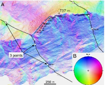
Fig. 5. (a) Color shaded DEM with examples of dip

measure-ments on the top fault scarp and on the two fault traces. (b)

Lower hemisphere stereographic projection used for the color shad-ing (COLTOP-3-D; Jaboyedoff et al., 2004a).

a strong simplification of this model is that it assumes that each element is independent of its neighboring ele-ments.

3.6 Step 5: Estimation of large unstable volumes using SLBL

The estimation of the volume of a landslide is a difficult task when only superficial data (a DEM and some airphotos) are available. A potential sliding surface must be defined, which implies that the geomorphologic features are extrapolated beneath the surface. The sloping local base level concept (SLBL, Jaboyedoff, 2004b) proposes a way to make such an extrapolation. The SLBL is a recent development of the XIX century geomorphologic concept of base level (Powell, 1875). The SLBL is a surface above which the volumes are liable to be affected by a gravitational movement. In 2-D, along a topographical profile, the SLBL can be explained as follow: for a spur located along an infinite slope, the SLBL corresponds to a line joining the top and the bottom of the spur. The SLBL is found by an iterative procedure of erosion active up to a limiting curvature: a point located above the mean of its two neighbors is replaced by this mean value ± a tolerance (Jaboyedoff et al., 2004b). In 3-D, the procedure is similar. The calculation is made by using the highest and the lowest values among the four direct neighboring points in a squared grid DEM. For the computation of the SLBL some points must be fixed otherwise the result is a flat to-pography (that corresponds to the old concept of base level). These fixed point can be rivers, crests or, like in the present case, the landslide contours (Jaboyedoff et al., 2004b). So two parameters are required from the geologist, according to his knowledge of the site: the landslide contours and the cur-vature of the sliding surface. Once a sliding plane has been

Fig. 6. Comparison of the measurement made on the DEM (a) and

in the field (b). Lower hemisphere stereographic projection of the average orientations of the discontinuities J1 and J2, the foliation and the topographical slope. Blue points: poles of the foliation planes.

defined, a volume can be calculated and then other parame-ters (e.g. mass, stress) can be deduced. We propose hereafter an example of estimation of a shear stress-index distribution on the SLBL surface in the area of the landslide. This in-dex is calculated by a simplified physical model (Jaboyedoff, 2004b): the shear stress on a surface element of the SLBL is composed of two types of contributions: 1) the shear stress due to the weight of rock directly above the element, 2) the contributions of the shear stress from the neighboring ele-ments. An element “pushes or pulls” its neighbors. This second contribution is assumed to be inversely proportional to the distance between two elements. Considering that this model is very simplistic, we have used the results qualita-tively to localize the most shear stressed areas on the SLBL.

4 Results

4.1 Step 0

It was not the aim of this step to get the most accurate and detailed DEM that the present photogrammetric technologies can provide (Mikhail et al., 2001). The elevation model was produced as simply as possible considering the size of the tar-get: an area of about 1 km2with a 600 m long and 50 m wide fault scarp at the top. A moderate resolution of 5m and only 6 ground control points were sufficient. Vertical airphotos and projections cannot depict precisely steep slopes (specif-ically more than 45◦_{) and usually other methods should be}

used (Buchroithner, 2002). Considering the resolution, the size of the targets and the mean slope of the mountainside (about 30◦) this limitation was not a critical issue. Never-theless, the DEM resolution influences the estimation of the dip of the slope (slope angle) and this point will be discussed hereafter.

4.2 Step 1

The interpretation of stereoscopic airphotos permits to iden-tify and map several types of features:

(6)

Fig. 7. Map of the areas where the kinematic conditions for sliding

on discontinuity J1 are satisfied (3 different dips of J1). The area in white indicates the potential toe of the main landslide.

a) Erosion features: the fault scarp at the top of the Opp-stadhornet is about 25 m high, 600 m long and 50 m wide (Fig. 4). Some small cliffs can be observed on the eastern part of the crest and will be used to delimit the source areas of potential block falls (Step 4).

b) Accumulation features: screes in the upper part and blocks in the lower part of the mountainside are indicators of rockfall activity (Step 4). Two ridges in the western lower part may help to locate basal sliding surfaces (Step 3).

c) Structural features: fault traces (Fig. 4) and bedding will be used in steps 2 and 3 to characterize the control of the geological structures on slope stability.

d) Hydrological features: in this case, the locations of rivers and ponds do not indicate that hey have an obvious ef-fect on the slope stability. Occurrence of springs in the lower part would have been a critical piece of information but it was not possible to get it from the initial data.

e) Man-made features: roads and buildings provide pre-liminary information about risk in the mass wasting area. 4.3 Step 2

Two main families of discontinuities have been character-ized using the DEM coincidentally with the faults traces and scarps identified in step 1. Their orientations (dip and dip di-rection) have been determined on the DEM using two types of measurements: a) direct measurement of the orientation of the fault scarp along the crest and b) two regional faults determined with the “3 points” method (Fig. 5).

The average slopes of the two families of discontinuities, J1 and J2, have been compared with the field measurements (Fig. 6). A good match is obtained between both sets of mea-surements. The dip values from the DEM are slightly lower

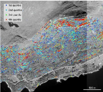
Fig. 8. Map of the areas where the kinematic conditions for a wedge

failure J1/J2 are satisfied (all the points in color). The color is an indicator of the probability to have such a wedge (red = high proba-bility). A relatively high density of hazardous wedges J1/J2 is likely along the eastern crest of the Oppsatdhornet.

than those the field. This is consistent with the trend to un-derestimate the dip of a slope when measuring it on a grid (Hodgson et al., 1995; Zhang et al., 1999). On the DEM, the average slope angle of the relief in the sliding area is 160◦/32◦.

4.4 Step 3

Comparing the orientations of the discontinuities obtained from step 2 with the topography, two different potentially hazardous structural arrangements have been identified: a) a planar sliding on J1, b) a failure on the wedges formed by J1 and J2.

Figure 7 is the map of the areas where the kinematic con-ditions for a sliding plane on J1 are satisfied. Due to the lack of information about the angle of internal friction and the fact that the dip of J1 has been measured mostly on the upper part of the DEM, but may vary lower in the mountainside, three different dips of J1 have been used: 30◦, 40◦and 50◦. The kinematic test is much less sensitive to the strike of J1 than to its dip. The average dip direction of 140◦has been used for all the tests. In the lower part, there are two elongated zones where the conditions are satisfied even for a steep dip of 50◦. It is in such areas that an outcropping sliding plane can be the most likely observed. This assumption has been confirmed by field investigations. Evidences of movements and basal detachment surfaces have been found in these areas (Blikra et al., 2001).

Figure 8 is the map of the areas where the conditions for a wedge failure J1/J2 are most likely satisfied. It shows a large zone on the crest of the mountain with a relatively high

(7)

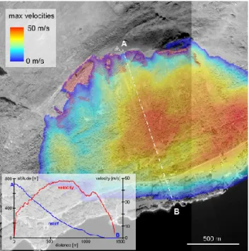
Fig. 9. Simulation of the maximal velocities of falling blocks (made

with CONEFALL). Critical angle = 32◦, velocity factor = 0.9, the dashed area is the source zone. In the inset, the relief and velocity profile along AB.

potential of hazardous wedges. Such an area can be an im-portant source of falling blocks.

4.5 Step 4

In Fig. 9, the potential source zones of falling blocks have been manually identified on the airphotos taking into consid-eration the potential density of wedges J1/J2 (step 3). Rock-falls may be problematic mainly in the eastern part of the Oppstadhornet mountainside (Fig. 9). The eastern part of the top ridge is steep (over 40◦) and the blocks can descend for more than 500 m (without considering the trees in the model). On the western flank, the average slope is inferior (about 30◦) and the blocks cannot reach high velocities.

The stress ratio calculation has been made for the sliding plane J1=140◦/40◦using Slopemap (G¨unther, 2003). All the slow sliding area on the western part of Oppstadhornet has a relatively high shear to normal stress ratio (Fig. 10). 4.6 Step 5

The SLBL method has been used to estimate the volume of the slow sliding mass on the western part of Oppstadhornet. The boundaries of the slide are deduced from the previous steps of this investigation: the top scarp and the faults form-ing the sides of the landslide from step 1, the foot from step 3 (the kinematics test for a planar sliding on J1). A very slightly concave sliding surface (=SLBL) has been chosen because of the morphology of the slope and the hard rock basement. Figure 11 shows the geometry of the sliding mass, limits and sliding plane, and the SLBL surface. The

differ-Fig. 10. Shear/normal stress ratio, using SLOPEMAP (G¨unther,

2003), on J1 produced by the weight of the rock at the vertical of the point (6= stress). Black dots = areas where the kinematics conditions for a sliding on J1=140◦/50◦are satisfied.

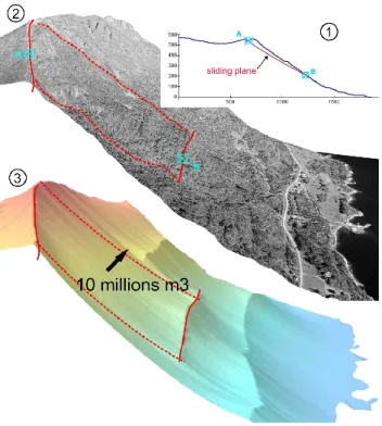
ence between the DEM and the SLBL surface provides the volume of the landslide: 10 million m3. This volume is in agreement with the estimations made by the field geologists (Blikra et al., 2001): 10–20 million m3.

On Fig. 12, the increasing shear stress-index towards the bottom of the landslide is in agreement with more advanced numerical models of stress analysis (Bhasin and Kaynia, 2004), even if the geometry has been strongly simplified. This slow landslide considered here as one slab is actually formed of at least four blocks (Blikra et al., 2001).

5 Discussion

This test of a preliminary assessment approach answers to most of the initial questions (geometry, mechanism and size of the phenomena). The agreement of these results with the field data collected are better than expected even if very sim-plified physical models have been used (i.e. no rheology or ballistic). These models require very few initial data. That is why they are useful at the beginning of an investigation.

Of course each step of this procedure has some limita-tions and drawbacks. During step 0, it is important that the resolution of the DEM fits the size and the slope angle of the targets (Hodgson et al., 1995; Zhang et al., 1999). The medium resolution adopted in this case was suitable for the main fault scarp but can lead to an underestimation of the slope of smaller and steep objects. The airphotos resolution limits the size of the objects that can be identified during step 1. With a resolution of about 0.5 m/pixel, only plurimetric blocks can be pointed. In step 2, even if both datasets are in very good agreement, the dips of the fault scarps determined from the DEM are systematically less steep than those mea-sured in the field (Fig. 6). This underestimation has a conse-quence on the results of the kinematic tests of step 3: some

(8)

Fig. 11. Volume estimation with a SLBL: 1) cross section along the

main landslide, 2) 3-D model with the contour of the landslide, 3) surface of the sloping local base level used to estimate the volume of the landslide.

pixels on known fault scarps have been missed by the tests. But the main key areas of the landslide, top scarps and foot, have been detected. Because of the simplistic physical mod-els used in step 4, the propagation and stress ratio maps have to be interpreted qualitatively. They provide an overview of the areas where rockfalls or planar sliding could be most problematic. The volume estimated in step 5 (about 10 mil-lion m3) is in agreement with the estimation made by Blikra et al. (2001; 10–20 millions m3), but is larger than the un-stable volume estimated by mechanical modeling (Bhashin and Kaynia, 2004; 5–7 millions m3). These discrepancies are principally caused by the fact that the sliding planes were placed at different depth in these studies. Nevertheless the volume estimated with the SLBL concept provides an order of magnitude coherent with the other estimations. The loca-tion of the maximal shear displacements from the 2-D me-chanical simulation of Bhashin and Kaynia (2004) is also in agreement with the higher value of the shear stress index for the sliding surface defined by the SLBL.

The procedure described here is only a first attempt and not a definitive mode of operation. We have tried to answer to our initial questions for our specific case. Similar proce-dures have been tested recently for other case studies, but each time they had to be adapted to the specificities of the site or of available data. Such a preliminary assessment does not intend to replace neither advanced numerical modeling, nor fieldwork. Ideally it should be done before fieldwork in order to optimize it.

Fig. 12. Distribution of the shear stress due to the overlaying rocks

on the SLBL surface.

6 Conclusions

Geographically referenced data will be increasingly avail-able to the scientific and public communities. This trend is particularly fast for the DEM because of the development of new technologies. For instance the lidar techniques, airborne or ground based, are able to provide DEMs with a sub-metric resolution. Such products are of course highly valuable for the stability analysis of a slope. Nevertheless, relatively few GIS tools have been developed to take advantage of these new data (Crosta and Agliardi, 2003; Dietrich and Montgomery, 1998; G¨unther, 2003; Jaboyedoff et al., 2004a; Pack et al., 1998). This case study was described to show the potential usefulness of such tools and the importance of developing new GIS tools that match the practical needs.

Edited by: G. B. Crosta Reviewed by: G. B. Crosta

References

Agliardi, F., Crosta, G., and Zanchi, A.: Structural constraints on deep-seated slope deformation kinematics, Engineering Geol-ogy, 59, 83–102, 2001.

Angelier, J.: Fault slip analysis and palaeostress reconstruction, in: Continental deformation, L. Hancock Paul, 53–100, 1994. Bashin, R. and Kaynia, A. M.: Static and dynamic simulation of a

700 m high rock slope in western Norway, Engineering Geology, 71, 213–226, 2004.

Blikra, L. H., Braathen, A., Anda, E., Stalsberg, K., and Longva, O.: Rock avalanches, gravitational bedrock fractures and neotec-tonics faults onshore northern West Norway: examples, regional distribution and triggering mechanisms, Report 2002.016 Geo-logical Survey of Norway (Trondheim), 48, 2002.

(9)

Blikra, L. H., Braathen, A., and Skurtveit, E.: Hazard evaluation of rock avalanches; the Baraldsnes – Oterøya area, Report 2001.108 Geological Survey of Norway (Trondheim), 33, 2001.

Buchroithner, M.: Creating the virtual Eiger North Face, ISPRS J PH, 57, 114–125, 2002.

Crosta, G. B. and Agliardi, F.: A methodology for physically based rockfall hazard assessment, in: Landslide risk assessment and mapping, edited by: Reichenbach, P. and Guzzetti, F., Nat. Haz. Earth Sys. Sci., 3, 407–422, 2003,

SRef-ID: 1684-9981/nhess/2003-3-407.

Cruden, D. M. and Varnes, D. J.: Landslide types and processes. In Landslides: investigation and mitigation, In: Transportation Research Board, edited by: Turner, A. K. and Schuster, R. L., Special Report No. 247, 36–75, 1996.

Dietrich, W. E. and Montgomery, D. R.: SHALSTAB: a digital terrain model for mapping shallow landslide potential (National Council of the Paper Industry for Air and Stream Improvement), 29, 1998.

Gokceoglu, C., Sonmez, H., and Ercanoglu, M.: Discontinuity con-trolled probabilistic slope failure risk maps of the Altindag (set-tlement) region in Turkey, Engineering Geology, 55, 277–296, 2000.

G¨unther, A.: SLOPEMAP: programs for automated mapping of geometrical and kinematical properties of hard rock hill slopes, Computer and Geosciences 29, 865–875, 2003.

G¨unther, A., Carstensen, A., and Pohl, W.:Automated sliding sus-ceptibility mapping of rock slopes, Nat. Haz. Earth Sys. Sci., 4, 95–102, 2004,

SRef-ID: 1684-9981/nhess/2004-4-95.

Guzzetti, F., Carrara, A., Cardinali, M., and Reichenbach, P.: Land-slides hazard evaluation: a review of current techniques and their application in a multi-scale study, Central Italy, Geomorphology, 31, 181–216, 1999.

Hodgson M.: What cell size does the computed slope/aspect angle represent?, PE&RS, 61, 5, 513–517, 1995.

Hoek, E. and Bray, J.: Rock slope engineering, revised third edition, E & FN Spon, London, 358, 1981.

Jaboyedoff, M.: Matterocking v 2.0. A program for detecting rock-slide instabilities, http://www.crealp.ch, 2002.

Jaboyedoff, M.: Conefall v 1.0. A program to estimate propa-gation zones of rockfall, based on cone methode (Quanterra), http://www.quanterra.ch, 2003.

Jaboyedoff, M., Philippossian, F., Mamin, M., Marro, C., and Rouiller, J.-D.: Distribution spatiale des discontinuit´es dans une falaise, Rapport de travail PNR31, VDF Publisher, Z¨urich, 90, 1996.

Jaboyedoff, M., Baillifard, F., Philippossian, F., and Rouiller, J.-D.: Assessing the fracture occurrence using the “Weighted fracturing density”: a step towards estimating rock instability hazard, Nat. Haz. Earth Sys. Sci., 4, 83–93, 2003,

SRef-ID: 1684-9981/nhess/2004-4-83.

Jaboyedoff, M., Baillifard, F., Couture, R., Locat, J., and Locat, P.: New insight of geomorphology and landslide prone area de-tection using DEM, in: Landslides Evaluation and stabilization, edited by: Lacerda, W. A., Ehrlich, M., Fontoura, A. B., and Sayo, A., Balkema, 199–205, 2004a.

Jaboyedoff, M., Baillifard, F., Couture, R., Locat, J., and Locat, P.: Toward preliminary hazard assessment using DEM topographic analysis and simple mechanic modeling, in: Landslides Evalu-ation and stabilizEvalu-ation, edited by: Lacerda, W. A., Ehrlich, M. Fontoura, A. B., and Sayo, A, Balkema, 191–197, 2004b. McKean, J. and Roering, J.: Objective landslide detection and

sur-face morphology mapping using high-resolution airborne laser altimetry, Geomorphology, 57, 331–351, 2004.

Mikhail, E. M., Bethel, J. S., and McGlone, J. C.: Modern Pho-togrammetry. Willey, 497, 2001.

Norrish, N. I. and Wyllie, D.: Rock slope stability analysis, in: Landslides – Investigation and mitigation, edited by: Turner, A. K. and Schuster, R. L., Transportation Research Board Special Report, 1996.

Pack, R. T., Tarboton, D. G., and Goodwin, C. N.: The SINMAP approach to terrain stability mapping, in: Proceedings; Eighth international congress; International Association for Engineering Geology and Environment; Theme 2, Engineering geology and natural hazards, edited by: Moore, D. P. and Hungr, O., 1157– 1165, 1998.

Robinson, P., Tveten, E., and Blikra, L. H.: A post-glacial bedrock failure at Oppstadhornet, Oterøya, More og Romsdal; a poten-tial major rock avalanche, Bulletin – Norges Geologiske Under-sokelse, 433, 46–47, 1997.

Soeters, R. and van Westen, C. J.: Slope instability recognition anal-ysis and zonation, In: Landslides: Investigation and Mitigation, edited by: Turner, A. K. and Schuster, R. L., Transportation Re-search Board National ReRe-search Council, Special Report 247, Washington D.C., 129–177, 1996.

van Westen, C. J.: Geo-information tools for landslide risk assess-ment: an overview of recent developments, in: Landslides Eval-uation and stabilization, edited by: Lacerda, W. A., Ehrlich, M., Fontoura, A. B., and Sayo, A., Balkema, 39–56, 2004.

Zhang, X., Drake, N., Wainwright, J., and Mulligan, M.: Compari-son of slope estimates from low resolution DEMs: scaling issues and a fractal method for their solution, Earth Surf. Process. Land-forms, 24, 763–779, 1999.