Evaluation of radar multiple scattering effects in Cloudsat configuration

(1)

HAL Id: hal-00302080

https://hal.archives-ouvertes.fr/hal-00302080

Submitted on 28 Aug 2006

HAL is a multi-disciplinary open access

archive for the deposit and dissemination of sci-entific research documents, whether they are pub-lished or not. The documents may come from teaching and research institutions in France or abroad, or from public or private research centers.

L’archive ouverte pluridisciplinaire HAL, est destinée au dépôt et à la diffusion de documents scientifiques de niveau recherche, publiés ou non, émanant des établissements d’enseignement et de recherche français ou étrangers, des laboratoires publics ou privés.

Evaluation of radar multiple scattering effects in

Cloudsat configuration

A. Battaglia, M. O. Ajewole, C. Simmer

To cite this version:

A. Battaglia, M. O. Ajewole, C. Simmer. Evaluation of radar multiple scattering effects in Cloudsat configuration. Atmospheric Chemistry and Physics Discussions, European Geosciences Union, 2006, 6 (4), pp.8125-8154. �hal-00302080�

(2)

ACPD

6, 8125–8154, 2006

Multiple scattering effects for Cloudsat

A. Battaglia et al. Title Page Abstract Introduction Conclusions References Tables Figures J I J I Back Close

Full Screen / Esc

Printer-friendly Version Interactive Discussion

EGU

Atmos. Chem. Phys. Discuss., 6, 8125–8154, 2006 www.atmos-chem-phys-discuss.net/6/8125/2006/ © Author(s) 2006. This work is licensed

under a Creative Commons License.

Atmospheric Chemistry and Physics Discussions

Evaluation of radar multiple scattering

e

ffects in Cloudsat configuration

A. Battaglia1, M. O. Ajewole2, and C. Simmer3

1

Meteorological Institute, University of Bonn, Bonn, Germany

2

Department of Physics, Federal University of Technology, Akure, Nigeria

3

Meteorological Institute, University of Bonn, Bonn, Germany

Received: 26 April 2006 – Accepted: 14 July 2006 – Published: 28 August 2006 Correspondence to: A. Battaglia (batta@uni-bonn.de)

(3)

ACPD

6, 8125–8154, 2006

Full Screen / Esc

EGU

Abstract

MonteCarlo simulations have been performed to evaluate the importance of multiple scattering effects in co- and cross-polar radar returns for 94 GHz radars in Cloudsat and airborne configurations. Thousands of vertically structured profiles derived from some different cloud resolving models are used as a test-bed. Mie theory is used 5

to derive the single scattering properties of the atmospheric hydrometeors. Multiple scattering effects in the cross polar channel (reflectivity enhancement) are particularly elusive, especially in airborne configuration. They can be quite consistent in satel-lite configurations, like Cloudsat, especially in regions of high attenuation and in the presence of highly forward scattering layers associated with snow and graupel parti-10

cles. When the cross polar returns are analysed, high LDR values appear both in space and in airborne configurations. The LDR signatures are footprints of multiple scattering effects since they cannot be explained by single scattering computations, even including non-spherical particles. We see these signatures confirmed by some experimental data collected during the Wakasa Bay experiment. Multiple scattering ef-15

fects can be important for Clousat applications like rainfall and snowfall retrievals since single scattering based algorithms will be otherwise burdened by positive biases.

1 Introduction

The Cloudsat mission, that will be launched early in 2006 as part of the NASA ESSP Program and of the A-train constellation, (Stephens et al.,2002), will fly the first space-20

borne millimeter wavelength radar. Among its main goals, the mission aims to detect snowfall from space, estimate how efficiently the atmosphere produces rain from con-densates and which percentage of terrestrial clouds produce rain, and to provide statis-tics on the vertical structure of clouds and light rain around the globe (e.g.Stephens,

2005). In this respect, Cloudsat observations can be seen as complementary to those 25

(4)

ACPD

6, 8125–8154, 2006

Full Screen / Esc

EGU

core satellite,http://gpm.gsfc.nasa.gov/) at lower frequencies and focused at observing and profiling situations with moderate to heavy rain. Compared to GPM-like radars, the higher frequency of the Cloudsat radar has the clear advantage of a better sensitivity to small cloud droplets and crystals, and of lower power, weight and size. This transfers into a better spatial resolution and a lower threshold of detection. In exchange, attenu-5

ation by atmospheric gases and by hydrometeors becomes an issue (Lhermitte,1987,

1990). L’Ecuyer and Stephens(2002) analyzed the importance of attenuation effects

when considering spaceborne radars at frequencies above 10 GHz. They implemented a very general optimal estimation-based algorithm for retrieving profiles of rainfall, ca-pable of accounting for different drop size/particle shape distribution and flexible to 10

include additional measurements from other sensors when available. When consider-ing a 94 GHz radar, their results show that the attenuation effects are too severe at rain rates greater than 1.5 mm/h. L’Ecuyer and Stephens (2002) concluded that only an additional constrain of the precipitation water path can raise this limit up to 10 mm/h.

However, their retrieval methodology is based on the fundamental assumption of 15

the validity of the single scattering (SS herafter) approximation for the radar equa-tion. Previous studies at lower frequencies (Marzano et al., 2003; Battaglia et al.,

2005;Kobayashi et al.,2005) have shown that multiple scattering (MS) effects become

relevant in space-borne configuration at 35 GHz at high scattering optical thickness (defined as the columnar integral of the scattering coefficient), e.g. associated with 20

large amounts of high-density ice particles. When reverting to 94 GHz the general in-crease of the SS albedo and of the extinction properties of all the hydrometeors will certainly favour the presence of MS effects. For a narrow beamwidth radar system, such as the one to be mounted on Cloudsat, a further increase in the forward scat-tering and consequently of the g parameter also implies an increase of MS effects. 25

On the other hand, higher frequencies allow for smaller antenna footprints (equal to 1×1 km2 for Cloudsat), that will generally reduce MS effects. It is therefore the main goal of this paper to investigate whether or not MS effects can be relevant to the variety of applications associated with the Cloudsat space-mission. Particular attention will be

(5)

ACPD

6, 8125–8154, 2006

Full Screen / Esc

EGU

focused on evaluating MS effects when profiles involving snow and low rain rates are considered. Strategies will be discussed that might get rid of MS-affected profiles in the retrieval procedure. Finally, the study will investigate under which conditions and in which radar signals will MS effects be revealed in air-borne field campaigns preliminary to the launch of Cloudsat. To do this the results of our simulations will be compared 5

with airborne observations acquired during the Wakasa Bay Experiment by a Cloudsat radar prototype.

2 MS effects in the radar signal

Battaglia et al.(2006a) have described a Monte Carlo-based simulator capable of

eval-uating single and multiple scattering apparent reflectivities for general radar configura-10

tions. The model has been employed to simulate signals for K_u and K_a band radars envisaged for the future GPM mission (seeBattaglia et al., 2006b). Here the same tool is applied to W −band radars. For the space-borne configuration we will use the Cloudsat parameters [altitude 705 km, beamwidth 0.1◦×0.1◦, minimum detection threshold (MDT hereafter) –26 dBZ] while the airborne configurations are chosen close 15

to those adopted for the NASA DC-8 and ER-2 cloud radars (seeSadowy et al.,1997;

Li et al.,2004) (altitude 20/6 km, beamwidth 0.8◦×0.8◦, MDT=–40 dBZ (but it should be

distance-dependent, as shown in Fig. 4 inLi et al.,2004)). The two airplane altitudes account for both stratospheric and tropospheric flights. In all cases nadir (downward-looking) radars are considered.

20

2.1 Uniform layer results

The Cloudsat space-borne configuration has been implemented first in the analytical model described in Battaglia et al. (2006a) to assess the importance of the second order of scattering (and thus indirectly of the MS) for an homogeneous layer with a prescribed SS albedo $, extinction coefficent k_ext and phase function. In the model 25

(6)

ACPD

6, 8125–8154, 2006

Full Screen / Esc

EGU

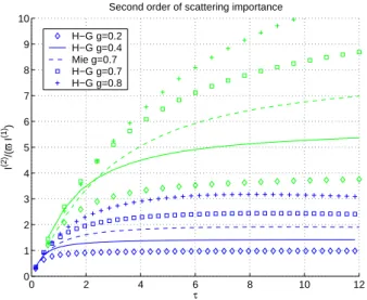
the transmitted radar pulse is perfectly collimated while in the receiving segment the (Cloudsat) antenna pattern is applied. Fig.1shows the ratio between the contribution of second order of scattering and the product of $ and the contribution of the first order of scattering. This quantity becomes more important with depth into the medium, with stronger extinguishing media (compare the blue and the green curves) and with phase 5

functions that are increasingly peaked (compare the different style curves). In Fig.1

Henyey-Greenstein phase functions with different values of the asymmetry parameter g are considered. For instance, for a medium with an extinction coefficient equal 0.6 km−1 (blue lines in Fig.1) and a phase function with g=0.7 (0.8), at large optical thickness (upper part of the panel), the second order of scattering contribution is almost 2.5 (3.2) 10

larger than for a medium with a phase function with g=0.2.

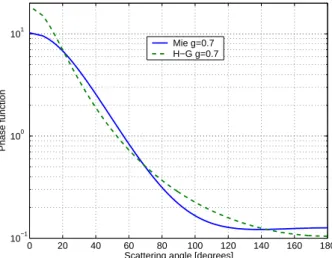
When reverting to phase functions computed with Mie theory the MS importance is slightly reduced. This is due to the different details of the phase functions (see also discussion in Sect. 4.2 in Battaglia et al.,2006a), which are depicted in Fig. 2. Note in particular the presence of the backscattering peak (better to say a backscat-15

tering plateau in this case) in the Mie-computed phase function that is absent in the always decreasing Henyey-Greenstein phase function and the higher forward peak in the Henyey-Greenstein phase function.

It is relevant that at 94 GHz g values around 0.7 are easily obtained in presence of ice hydrometeors when the scattering properties are computed with Mie theory (in 20

combination with the Maxwell and Garnett mixing rule, see Sect. 8 inBohren and Hu

ff-man,1983). The amplitude of the g parameter is typically enhanced when low density particles (like snow) are considered. However, some investigations of scattering prop-erties of ice/snow particles,Liu(2004), have revealed that, when non spherical shapes are considered, lower values of the g parameter are usually obtained. As a result of 25

the former discussion, when reverting to non-spherical shapes MS effects should be slightly reduced.

(7)

ACPD

6, 8125–8154, 2006

Full Screen / Esc

EGU

2.2 Inhomogeneous layer results

To be more realistic we have analyzed many different profiles extracted from different Cloud Resolving Models (CRM) simulations of different mesoscale systems (described in more detail inBattaglia et al.,2006b). Overpasses both of a space-borne and of an air-borne W −band radar over those systems have been considered. Some examples 5

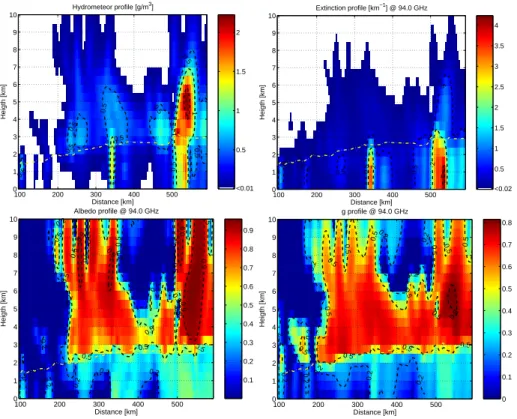
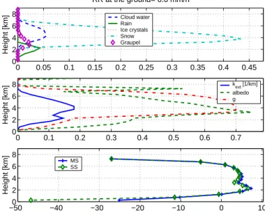
of the output of the simulator are shown in Figs.3–4. The total hydrometeor profile (the sum of all the hydrometeor species) is depicted in the top left panel of Fig.3with the dashed-dotted line indicating the freezing level. The cross section is characterized by different precipitating cells consisting of a variety of rain rates at the ground resulting from a mixture of cold and warm processes.

10

The associated SS properties are plotted in the other three panels of the same fig-ure. Extinction coefficients as high as 4 km−1 are found in heavy precipitation areas: this corresponds to a mean radiation path (the inverse of the extinction coefficient) of 250 m, which is much smaller than the Cloudsat footprint diameter. The SS albedo is always higher than 0.9 in the ice portion while it never exceeds 0.5 below the freezing 15

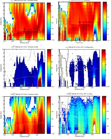
level (indicated by the dashed-dotted line). The asymmetry parameter ranges between 0.5 and 0.8 in the ice region while it can reach values as high as 0.4 when large rain-drops are present. The corresponding MS reflectivity, as sensed by W −band radars flying over the scene characterized by the scattering properties of Fig. 3, is shown in the top panels of Fig. 4. The left panels correspond to a CloudSat configuration, 20

the right panels to an airplane flying at 6 km altitude. In all the panels of Fig. 4 the dashed line represents the contour level at –26 dBZ/−40 dBZ for the SS reflectivity. When looking at the space-borne MS reflectivity (upper left panel) it is clear that, in SS configuration/regime, some of the regions close to the ground, due to attenuation problems, were below the MDT . However, they become detectable when MS signals 25

are considered. This is not true when considering the airborne configuration since in this case the SS and the MS contour levels are practically identical. The same conclu-sion can be made by looking at the central panels, that represent the MS enhancement

(8)

ACPD

6, 8125–8154, 2006

Full Screen / Esc

EGU

(i.e.∆ZMS≡ZMS−ZSS) in the two configurations (note that in these panels undetectable regions below –26 dBZ/−40 dBZ are blanked). While in the airborne configuration the MS enhancement is always lower than 2 dB, there are regions in the spaceborne con-figuration, where the effect can reach extremely high values. To have a better dynamic at low values the colorbar in the central left figure has been capped at 30 dB, but val-5

ues as high as 79 dB are actually reached in the region below the freezing level around 530 km. The radiation apparently sensed from those regions originates from waves scattered many times in the scattering ice layer above.

This is better demonstrated in the two panels of Fig.5. They correspond to two pro-files extracted from the precipitating cell of the cold front at 536 km (left) and 548 km 10

(right panels) with a rain rate at the ground equal respectively to 28.2 mm/h and 6.0 mm/h. This corresponds to a total optical thickness equal to 13.6 and 7.1 and to a scattering optical thickness equal to 7.8 and 4.8, respectively. Although quite different hydrometeor contents are present in the lower part of the two profiles, the MS reflectiv-ity profiles look quite similar (continuous-crossed lines in the bottom panels of Fig.5). 15

In contrast the SS profiles (dashed-diamond lines) are quite different with the heavy precipitating profile (left panel) characterized by a strong decrease due to higher atten-uation. The reason for this resides in both cases in the presence of a thick snow layer between about 8 and 2 km (top panel of Fig.5) characterized by very high SS albedo (around 0.95) and high asymmetry parameter (around 0.8, center panel of Fig.5). As 20

a result, what the radar is sensing at an apparent altitude less than 2 km is not a signal coming from the rain layer in that altitude but it is the MS signature of the upper layer. Obviously the interpretation of a MS signal like the one shown in the lower panels of Fig.5in terms of SS approximation will lead to completely wrong conclusions.

Another remarkable feature in the central left panel of Fig.4is the strong MS effect 25

present in the pixels close to the ground between 300 and 320 km. These pixels cor-respond practically to no hydrometeor content (see corcor-responding points in the top left panel of Fig.3). The hydrometeor scattering properties and MS/SS reflectivity vertical pattern for a profile in this region (corresponding to drizzle evaporating before hitting

(9)

ACPD

6, 8125–8154, 2006

Full Screen / Esc

EGU

the ground) are shown in Fig.6. The rain content reaches a maximum of 0.045 g/m3at 2 km (this corresponds to a RR=0.5 mm/h for a Marshall and Palmer drop size distri-bution) but then decreases to 0 at the ground (see the continuous line in the top panel of Fig.6). In this case the MS partially smoothens the transition at the cloud lowest boundary by spreading the cloud over a longer distance than its actual depth, an ef-5

fect well known in the lidar community (Bissonnette et al.,1995) and already indicated by the single-layer analyses performed in Sect. 5.3 of Battaglia et al. (2006a). This phenomenon has to be considered in the retrieval algorithms for vertical cloud profiles especially when cloud boundaries are sought.

The bottom panels of Fig. 4 represent the ratio between the cross and the copo-10

lar reflectivity signal, the LDR_hv, for space-borne and airborne configurations. In the space-borne configuration extraordinarily high values (up to –1.3 dB) can be noticed in some parts of the cross section. Since spherical particles are assumed in the study, these high LDR_hv values can only be due to MS effects. With only spherical particles assumed the first order of scattering cannot produce any cross-polarized signal. Since 15

we have simulated the emission of an h−polarized wave from the radar, the SS return can only be h−polarized. The return echo after more than one scattering event will tend to become more and more unpolarized. The LDR sensitivity to MS effects is greater than the reflectivity enhancement sensitivity to MS effects; in the spaceborne configu-ration, it can assume quite large values (around –15 dB at horizontal distances around 20

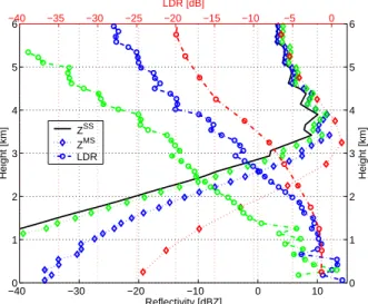
330 km in the bottom left panel of Fig.4) at altitudes around 5 km where practically no backscattering enhancement is apparent. This large sensitivity makes the effects of MS in the LDR signal visible in the air-borne configuration as well (see bottom right panel). Fig. 7 shows the reflectivity and LDR profiles at x=512 km for all three radar configurations (shown in three different colors). The SS reflectivity profile (continuous 25

black line) shows strong attenuation below 3.5 km. For the ER-2 configuration the MS reflectivity profile is practically the same (no significant difference between the green diamonds and the continuous black line) while MS enhancement becomes increasingly important moving to DC-8 (blue diamonds) and Cloudsat configuration (red diamonds).

(10)

ACPD

6, 8125–8154, 2006

Full Screen / Esc

EGU

Note that the profile is entirely detectable in the last two configurations only. For the ER-2, in the region below 1.1 km, the signal does not reach the MDT (and in fact this region is blanked in the center right and bottom right panels of Fig.4). The LDR pro-files (with scale at the top of the panel) are drawn in the undetectable regions as well. As before the MS effect is more evident in the Cloudsat configuration (red circles), 5

which has LDRs higher than −10 dB for all the pixels below 3.5 km. LDR values higher than −10 dB are found for the DC-8 and the ER-2 configurations below 2.6 and 1.4 km respectively as well. Finally, notice that, due to the high optical thickness, the results in the lower part are typically affected by Monte Carlo noise (especially when the highest vertical resolutions are employed).

10

2.3 General analyses

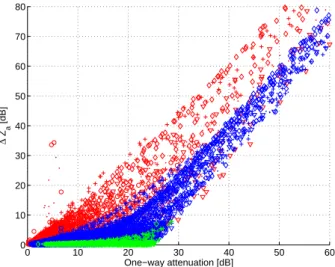
Hundreds of profiles extracted from different Cloud Resolving Models representing a cold front, a warm front, a tropical squall line over the Ocean and a convective system over the Amazon have been analyzed. In the former section, the reflectivity enhance-ment was often related to regions of high attenuation. This is more clearly illustrated in 15

Fig.8where each point corresponds to one simulated bin with a reflectivity above the

MDT . Generally the MS enhancement∆ZMS increases with the one way attenuation (which is proportional to the optical distance travelled inside the medium). When using logarithmic units, the detected radar reflectivity at a range r can be written as:

ZMS[0 → r]= ZSS[0 → r]+ ∆ZMS[0 → r] 20

= Ze[r] − A2−ways[0 → r]+ ∆Z[0 → r] (1)

where all quantities but the effective reflectivity Z_e are non local in the sense that they depend on the path between the radar (at range 0) and the bin (at range r). In Eq. (1) ∆ZMS

can be seen as a factor partially compensating for the two way attenuation. The plot in Fig.8has been clipped, i.e. some points with higher one way attenuation and 25

∆ZMS

(11)

ACPD

6, 8125–8154, 2006

Full Screen / Esc

EGU

Amazon convective system). As demonstrated in the comparisons of the two panels of Fig.5, in the presence of thick ice layers, the MS can become practically independent of the profile underneath so that it can enourmously increase when highly attenuating media are present.

Note however also those few points with high ∆ZMS at small attenuation. These 5

points derive from cloud border effects, as demonstrated when discussing Fig.6. The different radar configurations (red for Cloudsat, blue and green for airborne at 20 and 6 km altitude, respectively) lead to quite different reflectivity enhancements: while MS effects are obvious in the Cloudsat configuration in regions of high attenuation (red symbols) they are practically absent in the airborne configuration at 6 km (∆ZMS al-10

ways less than 7 dB, green symbols). But they are still important when an air-borne stratospheric platform is deployed (blue symbols).

In Fig. 8 a strong dispersion is noted in the scatterplot: for the same attenuation a wide range of∆ZMS results for each radar configuration. In particular, the presence of ice impacts the backscattering enhancement: with the same total optical thickness, 15

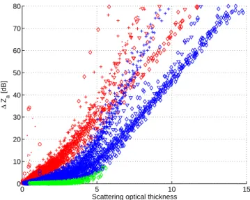
profiles rich in ice particles will have more MS effects. As demonstrated in Battaglia

et al. (2006b) this can be better explained by using as reference variable the scattering optical thickness (Fig.9). For a fixed scattering optical depth, there is now much less variability in ∆ZMS. At high scattering optical depth a clear separation between the MidAtlantic front systems (dots and cross symbols) and the tropical systems (diamonds 20

and triangles) is noticed. This relates to the different microphysics prevalent in both mesoscale systems, in particular the different re-partitioning of the ice portion between graupel and snow.

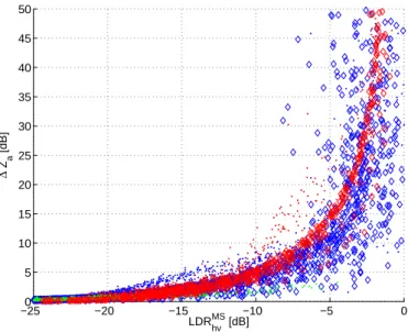
The discussion in Sect.2.2supports the idea that the LDR due to its high sensitivity can be used as an index for MS effects. This is demonstrated in Fig. 10 by including 25

the results for all different configurations. For instance, LDR values lower than –10, –15 or –20 dB always guarantee that MS reflectivity enhancement will stay below 10, 5 or 1.5 dB respectively..

(12)

ACPD

6, 8125–8154, 2006

Full Screen / Esc

EGU

effects have an impact on the derived rain rates profiles. Fig.11shows the reflectivity enhancement for profiles with rain rates at the ground below 10 mm/h when the Cloud-sat configuration is considered. The colour scale is graduated according to the rain rate at the ground. The plot provides a rough idea about how much MS can affect rain rate retrievals. In particular it shows that the extension to rain rates higher than 1.5 mm/h 5

needs to account for the presence of MS effects in the reflectivity signal. Even for lower rain rates, the MS reflectivity profile may differ noticebly from the SS reflectivity profile in the lower part. As an example Fig.12shows the SS/MS reflectivity profiles for a rain rate at the ground equal to 0.7 mm/h: the SS reflectivity is typically 4–5 dB lower than the MS reflectivity in the lower 3 km. Again we underline the fact that the MS effect is 10

driven by the presence of a strongly forward scattering ice layer. As a consequence similar considerations apply for snow-storm as well. Our results show that MS effects need to be accounted for when rainfall originating from multiphase processes with rates higher than 0.5 mm/h or snowfall are considered.

3 Air-borne campaigns and validation of MS effects

15

Air-borne campaigns have been carried out before the launch of the Cloudsat mission. The Wyoming Cloud Radar (see Galloway et al., 1997, and references therein) has provided the first polarimetric airborne observations at 95 GHz. Observations during field experiments in 1992 and 1994 show typical LDR features from the melting layer and from preferentially aligned ice crystals. During CRYSTAL-FACE (http://cloud1.arc.

20

nasa.gov/crystalface/) the Cloud Radar System (CRS, seeLi et al.,2004), operating at 94 GHz on board the NASA ER-2, acquired Doppler images over anvils generated by tropical maritime thunderstorms and over cirrus.

The data acquired by the Airborne Cloud Radar (ACR) sensor, mounted on a NASA P-3 aircraft, and flown over the Sea of Japan, the Western Pacific Ocean, and the 25

Japanese Islands in the Wakasa Bay Field Campaign in January and February 2003 are found to be of particular interest for this study. This data set (plublicly available in

(13)

ACPD

6, 8125–8154, 2006

Full Screen / Esc

EGU

netCDF via FTP,Stephens and Austin.,2004) includes 94 GHz co- and cross-polarized radar reflectivities. Flight legs were usually flown around 6400 m above mean sea level. The ACR has a beamwidth of 0.8◦and was usually operated with a vertical resolution of 120 m. In this database some interesting cases have been found with enhanced values of LDRs; examples are provided in Figs.13–14.

5

In both panels, the bright band can be seen as an horizontal strip with LDR values around –12 to –15 dB located at about 2.5 and 1.5 km. These bright band features are in agreement with former melting layer observations at vertical incidence during the Winter Icing and Storms Project (seeGalloway et al., 1997). However much higher values of LDR (up to about 0 dB) are observed in coincidence in strongly attenuating 10

regions (as indicated by the low surface echo in the reflectivity panels). These features do not seem to be produced by a low signal to noise ratio (a problem that was present in the dataset of the APR-2, seeIm,2003). In the analyses we have excluded all pixels with cross polar reflectivity lower than –50 dBZ; they appear blank in Figs.13–14. By so doing we avoided the presence of possible high LDR values at cloud boundaries 15

(like in the upper right corner in Fig.13). These LDR features can hardly be explained from the SS point of view.Wolde and Vali(2001a,b) discuss polarimetric signatures as observed by the Wyoming airborne cloud radar at close distance which are certainly not affected by propagation and MS effects. They report observations of high LDR with graupel in a cumulus congestus; however these values do not exceed –6 dB at 20

side view and –9 dB when nadir looking (see their Fig. 6). The fuzzy logic algorithm described by Aydin and Singh (2004) assumes –5 dB as the highest possible value for LDR detectable from graupel particles (considering all incidence directions). The frequency of occurences of high LDR signatures in the Wakasa dataset is remarkable; if interpreted in terms of MS signal, the explanation seems straightforward and the 25

(14)

ACPD

6, 8125–8154, 2006

Full Screen / Esc

EGU

4 Conclusions

The relevance of MS effects has been evaluated for the Cloudsat configuration both for reflectivity enhancement and for the LDR signal. The simplified study conducted on a uniform layer reveals that large scattering optical thickness and asymmetry parameters are key factors in enhancing MS effects.

5

A typical midlatitude scenario has been analysed in detail to understand the rela-tive importance of MS reflectivity enhancement and LDR in vertically inhomogeneous profiles containing a mixture of hydrometeors. The intercomparison between Cloudsat and an airborne tropospheric airplane configuration reveals that the effect of the reflec-tivity enhancement is not detectable in the airborne configuration while it can be pretty 10

large in regions of high attenuation for the spaceborne configuration. High LDR val-ues, however, appear in both configurations. These distinctive LDR signatures of MS seems confirmed by experimental data collected during the Wakasa Bay experiment.

The analysis of a wide range of profiles shows the strong correlation between the attenuation (and even more the scattering optical depth) and the MS reflectivity en-15

hancement. Crucial to this correlation between attenuation and MS enhancement is the role played by the the amount and the type of ice hydrometeors involved. Even for very low rain rates the presence of snow crystals or graupel particles aloft may induce MS reflectivity enhancements in the rain layer underneath. This has to be taken into account when profiling algorithms are employed. In fact the MS effect can be inter-20

preted as an effective reduction of the two-way attenuation by an amount equal to the MS enhancement. As a result rainfall estimates based on the SS approximation are believed to be burdened by positive biases.

If available, the measurement of the cross polarized signal can enormously help to detect areas potentially affected by MS enhancement since there is a clear relationship 25

between this quantity and LDR values. More studies on this topic are necessary to cor-roborate our results, especially by exploiting airborne polarized radar data derived in field caimpagns. Due to the importance of SS scattering properties, a sensitivity study,

(15)

ACPD

6, 8125–8154, 2006

Full Screen / Esc

EGU

including a better description of the ice segment of the cloud, will be conducted. When switching to non spherical ice particles the asymmetry parameter and the extinction coefficient -two key parameters affecting MS- generally are far apart from the equivol-ume sphere approximation counterparts (seeLiu,2004). The non spherical shape of raindrops is believed to play a minor role in modifying the SS properties.

5

Acknowledgements. M. Ajewole is grateful to the Alexander von Humboldt Foundation, the

University of Bonn and the Federal University of Technology of Akure for the research visit to Germany. The authors wish to thank all the Airborne Cloud Radar (ACR) team, which made available the dataset of 94 GHz co- and cross-polarized radar reflectivities collected during the Wakasa-Bay field experiment (seehttp://nsidc.org/data/nsidc-0212.html).

10

References

Aydin, K. and Singh, J.: Cloud Ice Crystal Classification Using a 95-GHz Polarimetric Radar, J. Atmos. Ocean Technol., 21, 1679–1688, 2004. 8136

Battaglia, A., Ajewole, M. O., and Simmer, C.: Multiple scattering effects due to hydrometeors on precipitation radar systems, Geophys. Res. Lett., 32, L19801,

15

doi:10.1029/2005GL023810, 2005. 8127

Battaglia, A., Ajewole, M. O., and Simmer, C.: Evaluation of radar multiple scattering effects from a GPM perspective. Part I: model description and validation, J. Appl. Meteorol., in press, 2006a. 8128,8129,8132

Battaglia, A., Ajewole, M. O., and Simmer, C.: Evaluation of radar multiple scattering effects

20

from a GPM perspective. Part II: model results, J. Appl. Meteorol., in press, 2006b. 8128,

8130,8134

Bissonnette, L. R., Bruscaglioni, P., Ismaelli, A., Zaccanti, G., Cohen, A., Benayahu, Y., Kleiman, M., Egert, S., Flesia, C., Schwendimann, P., Starkov, A. V., Noormohammadian, M., Oppel, U. G., Winker, D. M., Zege, E. P., Katsev, I. L., and Polonski, I. N.: Lidar multiple

25

scattering from clouds, Appl. Phys. B, 60, 355–362, 1995. 8132

Bohren, C. F. and Huffman, D. R.: Absorption and Scattering of Light by Small Particles, John Wiley & Sons, New York, 1983. 8129

(16)

ACPD

6, 8125–8154, 2006

Full Screen / Esc

EGU

Galloway, J., Pazmany, A., Mead, J., McIntosh, R. E., Leon, D., French, J., Kelly, R., and Vali, G.: Detection of Ice Hydrometeor Alignment Using an Airborne W-band Polarimetric Radar, J. Atmos. Ocean Technol., 14, 3–12, 1997. 8135,8136

Im, E.: APR-2 Dual-Frequency Airborne Radar Observations, Wakasa Bay, Japan, boulder, CO: National Snow and Ice Data Center, Digital media, 2003. 8136

5

Kobayashi, S., Tanelli, S., and Im, E.: Second-order multiple-scattering theory associated with backscattering enhancement for a millimeter wavelength weather radar with a finite beam width, Radio Sci., 40, RS6015, doi:10.1029/2004RS003219, 2005. 8127

L’Ecuyer, T. S. and Stephens, G. L.: An Estimation-Based Precipitation Retrieval Algorithm for Attenuating Radars, J. Appl. Meteorol., 41, 272–285, 2002. 8127

10

Lhermitte, R.: A 94 GHz Doppler Radar for Cloud Observation, J. Atmos. Ocean Technol., 4, 36–48, 1987. 8127

Lhermitte, R.: Attenuation and Scattering of Millimeter Wavelength Radiation by Clouds and Precipitation, J. Atmos. Ocean Technol., 7, 464–479, 1990. 8127

Li, L., Heymsfield, G. M., Racette, P. E., Tian, L., and Zenker, E.: A 94-GHz Cloud Radar

15

System on a NASA High-Altitude ER-2 Aircraft, J. Atmos. Ocean Technol., 21, 1378–1388., 2004. 8128,8135

Liu, Q.: Approximation of Single Scattering Properties of Ice and Snow Particles for High Mi-crowave Frequencies, J. Atmos. Sci., 61, 2441–2456, 2004. 8129,8138

Marzano, F. S., Roberti, L., Di Michele, S., Mugnai, A., and Tassa, A.: Modeling of apparent

20

radar reflectivity due to convective clouds at attenuating wavelenghts, Radio Sci., 38(1), 1002, doi:10.1029/2002RS002613, 2003. 8127

Sadowy, G. A., McIntosh, R. E., Dinardo, S. J., Durden, S. L., Edelstein, W. N., Li, F. K., Tanner, A. B., Wilson, W. J., Schneider, T. L., and Stephens, G. L.: The NASA DC-8 airborne cloud radar: design and preliminary results, in: Proceedings of IGARSS ’97, 4, 1466–1469, 1997.

25

8128

Stephens, G. L.: Cloud Feedbacks in the Climate System: A Critical Review, J. Climate, 18, 237–273, 2005. 8126

Stephens, G. L. and Austin., R. T.: Airborne Cloud Radar (ACR) Reflectivity, Wakasa Bay, Japan, boulder, CO: National Snow and Ice Data Center. Digital media, 2004. 8136

30

Stephens, G. L., Vane, D. G., Boain, R. J., Mace, G. G., Sassen, K., Wang, Z., Illingworth, A. J., O’Connor, E. J., Rossow, W. B., Durden, S. L., Miller, S. D., Austin, R. T., Benedetti, A., Mitrescu, C., and Team, T. C. S.: The CLOUDSAT mission and the A-train, Bull. Am.

(17)

ACPD

6, 8125–8154, 2006

Full Screen / Esc

EGU

Meteorol. Soc., 83, 1771–1790, 2002. 8126

Wolde, M. and Vali, G.: Polarimetric Signatures from Ice Crystals Observed at 95 GHz in Winter Clouds. Part I: Dependence on Crystal Form, J. Atmos. Sci., 58, 828–841, 2001a. 8136

Wolde, M. and Vali, G.: Polarimetric Signatures from Ice Crystals Observed at 95 GHz in Winter Clouds. Part II: Frequencies of Occurrence, J. Atmos. Sci., 58, 842–849, 2001b. 8136

(18)

ACPD

6, 8125–8154, 2006

Full Screen / Esc

Printer-friendly Version Interactive Discussion EGU 0 2 4 6 8 10 12 0 1 2 3 4 5 6 7 8 9 10

Second order of scattering importance

τ I (2) /( ϖ I (1) ) H−G g=0.2 H−G g=0.4 Mie g=0.7 H−G g=0.7 H−G g=0.8

Fig. 1. Relevance of the second order of scattering (defined as the ratio between the intensity relative the second order of scattering and the product of the SS albedo and the SS intensity) as a function of the optical thickness. Blue and green lines correspond to a uniform layer with extinction coefficient equal to 0.6 and 2.4 km−1

(19)

ACPD

6, 8125–8154, 2006

Full Screen / Esc

Printer-friendly Version Interactive Discussion EGU 0 20 40 60 80 100 120 140 160 180 10−1 100 101

Scattering angle [degrees]

Phase function

Mie g=0.7 H−G g=0.7

(20)

ACPD

6, 8125–8154, 2006

Full Screen / Esc

Printer-friendly Version Interactive Discussion EGU Distance [km] Heigth [km] Hydrometeor profile [g/m3_] 0.5 0.5 0.5 0.5 0.5 0.5 0.5 0.5 0.5 1 1 1 2 100 200 300 400 500 0 1 2 3 4 5 6 7 8 9 10 <0.01 0.5 1 1.5 2 Distance [km] Heigth [km] Extinction profile [km−1_{] @ 94.0 GHz} .5 _0.5 0.5 0.5 0.5 0.5 2 2 4 100 200 300 400 500 0 1 2 3 4 5 6 7 8 9 10 <0.02 0.5 1 1.5 2 2.5 3 3.5 4 Distance [km] Heigth [km] Albedo profile @ 94.0 GHz .2 _0.2 0.2 0.2 0.2 0.2 0.2 0.2 0.2 0.2 0.2 0.2 0.2 .5 0.5 0.5 0.5 0.5 0.5 0.5 0.5 0.5 0.5 0.5 0.5 0.9 0.9 0.9 0.9 0.9 100 200 300 400 500 0 1 2 3 4 5 6 7 8 9 10 0.1 0.2 0.3 0.4 0.5 0.6 0.7 0.8 0.9 Distance [km] Heigth [km] g profile @ 94.0 GHz 0.2 0.2 0.2 0.2 0.2 0.2 0.2 0.2 0.2 0.2 2 0.5 0.5 0.5 0.5 0.5 0.5 0.5 0.5 0.5 0.5 0.5 0.5 0.5 0.8 100 200 300 400 500 0 1 2 3 4 5 6 7 8 9 10 0 0.1 0.2 0.3 0.4 0.5 0.6 0.7 0.8

Fig. 3. Cross section of a MidAtlantic Cold Front: hydrometeor content in g/m3 (top left),

extinction coefficient in km−1 (top right), SS albedo (bottom left) and asymmetry parameter (bottom right) profiles. The yellow dash-dotted line corresponds to the freezing level altitude.

(21)

ACPD

6, 8125–8154, 2006

Full Screen / Esc

Printer-friendly Version Interactive Discussion EGU Distance [km] Heigth [km] Za MS_{[dBZ] @ 94.0 GHz, Cloudsat config.} −26 −26 100 200 300 400 500 0 1 2 3 4 5 6 7 8 9 10 <−50 −40 −30 −20 −10 0 10 Distance [km] Heigth [km] ZaMS [dBZ] @ 94.0 GHz, ER−2 configuration −40 −40 −40 −40 −40 −40 −40 −40 −40 −40 −40 −40 −40 −40 −40 −40 −40 100 150 200 250 300 350 400 450 500 550 0 1 2 3 4 5 6 <−50 −40 −30 −20 −10 0 10 Distance [km] Heigth [km] ∆ Za MS_{[dB] @ 94.0 GHz, Cloudsat config.} −26 −26 6 − −26 100 200 300 400 500 0 1 2 3 4 5 6 7 8 9 10 <0.2 5 10 15 20 25 30 Distance [km] Heigth [km] Δ Z a [dB] @ 94.0 GHz, ER−2 configuration −40 −40 −40 −40 −40 −40 −40 −40 −40 −40 −40 −40 −40 −40 −40 −40 100 200 300 400 500 0 1 2 3 4 5 6 <0.05 1 2 3 4 5 6 Distance [km] Heigth [km] LDRhv MS_{[dB] @ 94.0 GHz, Cloudsat config.} −26 −26 −2 −26 100 200 300 400 500 0 1 2 3 4 5 6 7 8 9 10 <−50 −40 −30 −20 −10 0 Distance [km] Heigth [km] LDRhv MS_{[dB] @ 94.0 GHz, ER−2 config.} −40 −40 −40 −40 −40 −40 −40 −40 −40 −40 −40 −40 −40 −40 −40 −40 −40 100 200 300 400 500 0 1 2 3 4 5 6 <−50 −40 −30 −20 −10 0

Fig. 4. Radar quantities simulated in correspondence to the cross section of a MidAtlantic Cold Front depicted in Fig.3. Top panels: MS reflectivity; central panels: reflectivity enhancement due to MS; bottom panels: LDRhv. The panels on the left correspond to CloudSat

space-borne configuration (beamwidth 0.1◦, altitude 705 km) the panels on the right to ER-2 air-borne configuration (beamwidth 0.8◦, altitude 6 km).

(22)

ACPD

6, 8125–8154, 2006

Full Screen / Esc

Printer-friendly Version Interactive Discussion EGU −40 −30 −20 −10 0 10 0 2 4 6 8 Height [km] MS SS 0 0.5 1 1.5 2 0 2 4 6 8 RR at the ground= 28.2 mm/h Height [km] Cloud water Rain Ice crystals Snow Graupel 0 0.5 1 1.5 2 2.5 3 3.5 4 0 2 4 6 8 Height [km] k_ext [1/km] albedo g −40 −30 −20 −10 0 10 0 2 4 6 8 Height [km] MS SS 0 0.5 1 1.5 2 0 2 4 6 8 RR at the ground= 6.0 mm/h Height [km] Cloud water Rain Ice crystals Snow Graupel 0 0.2 0.4 0.6 0.8 1 1.2 1.4 0 2 4 6 8 Height [km] k_ext [1/km] albedo g

Fig. 5. Heavy and medium rain case extracted from the Cold Front simulation. Top panels: hydrometeor content in g/m3. Central panels: scattering properties. Bottom panels: ZaMSand

(23)

ACPD

6, 8125–8154, 2006

Full Screen / Esc

Printer-friendly Version Interactive Discussion EGU −500 −40 −30 −20 −10 0 10 2 4 6 8 Height [km] MS SS 0 0.05 0.1 0.15 0.2 0.25 0.3 0.35 0.4 0.45 0 2 4 6 8 RR at the ground= 0.0 mm/h Height [km] Cloud water Rain Ice crystals Snow Graupel 0 0.1 0.2 0.3 0.4 0.5 0.6 0.7 0 2 4 6 8 Height [km] k ext [1/km] albedo g

Fig. 6. Profile with evaporating drizzle close to the ground extracted from the Cold Front simu-lation. Top panels: hydrometeor content in g/m3. Central panels: scattering properties. Bottom panels: ZaMSand Z

SS

(24)

ACPD

6, 8125–8154, 2006

Full Screen / Esc

Printer-friendly Version Interactive Discussion EGU −400 −30 −20 −10 0 10 1 2 3 4 5 6 Reflectivity [dBZ] Height [km] ZSS ZMS LDR −40 −35 −30 −25 −20 −15 −10 −5 0 0 1 2 3 4 5 6 LDR [dB] Height [km]

Fig. 7. SS (continuous black line) and MS (diamond-dotted line) reflectivity and LDR (circle-dashed line) profile extracted from the Cold Front simulation at x=512 km in Cloudsat (red colour), DC-8 (blue) and ER-2 (green) configurations.

(25)

ACPD

6, 8125–8154, 2006

Full Screen / Esc

Printer-friendly Version Interactive Discussion EGU 0 10 20 30 40 50 60 0 10 20 30 40 50 60 70 80 ∆ Za [dB] One−way attenuation [dB]

Fig. 8. Scatterplot of one way attenuation versus MS enhancement. Different symbols

corre-spond to different CRM (triangles for the squall line, diamonds for the LBA convection, crosses for the warm front, dots and circle for the Cold front), different colours to different radar config-urations [red: Cloudsat configuration, blue: DC-8 configuration (i.e. 0.8◦beamwidth and 20 km flight altitude), green: ER-2 configuration (i.e. 0.8◦beamwidth and 6 km flight altitude).

(26)

ACPD

6, 8125–8154, 2006

Full Screen / Esc

Printer-friendly Version Interactive Discussion EGU 0 5 10 15 0 10 20 30 40 50 60 70 80 ∆ Za [dB]

Scattering optical thickness

Fig. 9. Scattering optical thickness versus MS enhancement. Different symbols correspond to different CRMs, different colours to different radar configurations as described in caption of Fig.8.

(27)

ACPD

6, 8125–8154, 2006

Full Screen / Esc

Printer-friendly Version Interactive Discussion EGU −250 −20 −15 −10 −5 0 5 10 15 20 25 30 35 40 45 50 LDR hv MS_[dB] Δ Za [dB]

Fig. 10. Scatterplots of LDR values versus MS reflectivity enhancement for the space-borne (red colour), the stratosphere DC-8/ER-2 airborne configurations (blue and green colour). Dif-ferent symbols correspond to difDif-ferent CRMs: diamonds for the LBA convection and dots for the Cold front.

(28)

ACPD

6, 8125–8154, 2006

Full Screen / Esc

Printer-friendly Version Interactive Discussion EGU −25 −20 −15 −10 −5 0 5 10 0 5 10 15 20 25 30 35 40 Z a [dBZ] ∆ Za MS [dBZ] 0.1 2 3.9 5.9 7.8 9.8

Fig. 11. Scatterplot of ZaMSversus MS reflectivity enhancement in Cloudsat configuration as a

function of the rain rate at the ground (as readable in the colorbar). Different symbols corre-spond to different CRM simulations.

(29)

ACPD

6, 8125–8154, 2006

Full Screen / Esc

Printer-friendly Version Interactive Discussion EGU −50 0 5 10 2 4 6 8 Height [km] MS SS 0 0.2 0.4 0.6 0.8 1 0 2 4 6 8 RR at the ground= 0.7 mm/h Height [km] Cloud water Rain Ice crystals Snow Graupel 0 0.2 0.4 0.6 0.8 1 0 2 4 6 8 Height [km] k ext [1/km] albedo g

Fig. 12. Low rain case extracted from the Cold Front simulation. Top panels: hydrometeor content in g/m3. Central panels: scattering properties. Bottom panels: ZaMSand Z

SS

a profiles in

(30)

ACPD

6, 8125–8154, 2006

Full Screen / Esc

EGU

UTC [hour]

Altitude [km]

Co−polar reflectivity date=20030123.094400

10.65 10.7 10.75 10.8 0 0.5 1 1.5 2 2.5 3 3.5 4 4.5 5 −40 −30 −20 −10 0 10 20 30 surface echo UTC [hour] Altitude [km] LDR [dB] date=20030123.094400 10.65 10.7 10.75 10.8 0 0.5 1 1.5 2 2.5 3 3.5 4 4.5 5 −50 −45 −40 −35 −30 −25 −20 −15 −10 −5 0

Fig. 13. Detail of the copolar reflectivity and the LDR as measured by the ACR during the Wakasa Bay Experiment on the 23 January 2003.

(31)

ACPD

6, 8125–8154, 2006

Full Screen / Esc

EGU

UTC [hour]

Altitude [km]

Co−polar reflectivity date=20030121.025321

3.43 3.435 3.44 3.445 3.45 3.455 3.46 3.465 3.47 0 0.5 1 1.5 2 2.5 3 3.5 4 4.5 5 −40 −30 −20 −10 0 10 20 30 40 surface echo UTC [hour] Altitude [km] LDR [dB] date=20030121.025321 3.43 3.435 3.44 3.445 3.45 3.455 3.46 3.465 3.47 0 0.5 1 1.5 2 2.5 3 3.5 4 4.5 5 −50 −45 −40 −35 −30 −25 −20 −15 −10 −5 0

Fig. 14. Detail of the copolar reflectivity and the LDR as measured by the ACR during the Wakasa Bay Experiment on the 21 January 2003.