HAL Id: hal-02357497
https://hal.univ-lorraine.fr/hal-02357497
Submitted on 10 Nov 2019
HAL is a multi-disciplinary open access
archive for the deposit and dissemination of sci-entific research documents, whether they are pub-lished or not. The documents may come from teaching and research institutions in France or abroad, or from public or private research centers.
L’archive ouverte pluridisciplinaire HAL, est destinée au dépôt et à la diffusion de documents scientifiques de niveau recherche, publiés ou non, émanant des établissements d’enseignement et de recherche français ou étrangers, des laboratoires publics ou privés.
High-precision in situ silicon isotopic analyses by
multi-collector secondary ion mass spectrometry in
olivine and low-calcium pyroxene
Johan Villeneuve, Marc Chaussidon, Yves Marrocchi, Zhengbin Deng, E.
Bruce Watson
To cite this version:
Johan Villeneuve, Marc Chaussidon, Yves Marrocchi, Zhengbin Deng, E. Bruce Watson. High-precision in situ silicon isotopic analyses by multi-collector secondary ion mass spectrometry in olivine and low-calcium pyroxene. Rapid Communications in Mass Spectrometry, Wiley, 2019, 33 (20), pp.1589-1597. �10.1002/rcm.8508�. �hal-02357497�
High-precision In situ silicon isotopic analyses by MC-SIMS in olivine and low-Ca pyroxene
1 2
Johan Villeneuve
1,*, Marc Chaussidon
2, Yves Marrocchi
1, Zhengbin Deng
2, and E. Bruce
3Watson
3 41
Centre de Recherches Pétrographiques et Géochimiques, CNRS UMR 7358, Université de Lorraine, 5
15 rue Notre-Dame des Pauvres, Vandœuvre-lès-Nancy, 54501 France 6
2
Institut de Physique du Globe de Paris, Université Sorbonne Paris Cité, CNRS UMR 7154, 1 rue 7
Jussieu, Paris, 75238 Paris France 8
3
Department of Earth and Environmental Sciences, Rensselaer Polytechnic Institute, Troy, NY 12180 9
USA 10
*Corresponding author, [email protected] 11
Abstract
12 13
Rationale:
High-precision determination of silicon isotopes can be achieved by in situ multi-collector 14secondary ion mass spectrometry. The analyses accuracy is however sensitive to ion yields and 15
instrumental mass fractionations (IMFs) induced by the analytical procedure. These effects vary from 16
an instrument to another, with the analytical settings, and with the composition and nature of the 17
sample. Because ion yields and IMF effects are not predictable and rely on empirical calibrations, 18
high-accuracy analyses require suitable sets of standards. 19
Methods:
Here, we document calibrations of ion yields and matrix effects in a set of 23 olivine 20standards and 3 low-Ca pyroxene for silicon isotopic measurements in both polarities using Caméca 21
IMS 1270 E7 and IMS 1280 HR2 ion probes set with the cesium or radiofrequency (RF) source. 22
Results:
Silicon ion yields show (i) strong variations with the chemical composition, and (ii) an 23opposite behavior between the secondary positive and negative polarities. The magnitude of IMF 24
along the fayalite-forsterite (olivine) series shows a complex behavior, increasing overall by ≈7‰ 25
(secondary positive) and ≈15‰ (secondary negative) with increasing olivine Mg#. A drastic change in 26
olivine IMF occurs at Mg# ≈ 70 in both polarities. The magnitude of IMF for low-Ca pyroxene from 27
Mg# = 70-100 is almost constant in both polarities, i.e. ≈0.1‰ in secondary positive and ≈0.15‰ in 28
secondary negative. Analytical uncertainties on individual analyses were ±0.05–0.15‰ (2 S.E.) with 29
both sources, and external errors for each standard material were ≈ ±0.05–0.5‰ (2 S.E.) with the Cs 30
source and ≈ ±0.03–0.15‰ (2 S.E.) with the RF source. 31
Conclusions: The IMF effect of Si isotopes in silicates shows complex behaviors that vary with the
32
chemistry and the settings of the instrument. We developed a suitable set of standards in order to 33
perform high-accuracy in situ measurements of Si isotopes in olivine and low-Ca pyroxene 34
characterized by varying chemical compositions by MC-SIMS. 35
36
Keywords: Secondary ion mass spectrometer, silicon isotopes, ion yield, matrix effects
37 38 39 40 41 42 43 44 45 46 47 48 49 50
Introduction
51
Natural stable isotopic variations result from various processes that affect geological materials during 52
their formation. Because H, C, N, O, and S commonly show large isotopic fractionations, they have 53
been widely used in Earth and planetary sciences during the last half-century. Owing to recent 54
considerable improvements in analytical methods, high-precision isotopic measurements of a large 55
number of typically less-fractionated elements (Mg, Si, Fe, Cr, Zn, etc.) are now possible, providing 56
insights into various processes such as evaporation and condensation during planetary formation1, 57
igneous differentiation2, or metal-silicate fractionation3. Among the instruments allowing in situ 58
isotopic analyses, the latest generation of ions probes, allowing multi-collector secondary ion mass 59
spectrometry (MC-SIMS), is the most versatile with unique advantages: (i) high spatial resolution (5– 60
20 μm beam diameter and 1–2 μm depth); (ii) high sensitivity, allowing detection limits below the 61
ppm level for most elements; (iii) high mass-resolution analysis, thus removing most isobaric 62
interferences; and (iv) a good level of analytical precision, usually better than 1‰ at 2σ depending on 63
the element analyzed4–7. These advantages make ion probes powerful tools for studying isotopic 64
fractionations in complex mineralogical assemblages and zoned minerals. Regardless of the 65
technique used, high-precision in situ isotopic analyses have always been challenging and rely on the 66
use of suitable reference materials. Ion probes measurements can be particularly sensitive to 67
differences in ion yields between elements and to mass-dependent instrumental isotopic 68
fractionation. This latter effect is usually referred to as instrumental mass fractionation (IMF) and 69
corresponds to the difference between the natural isotopic composition of a sample and the value 70
measured with the ion probe. Ion yield and IMF essentially depend on the physics of the mass 71
spectrometer, the analytical settings, and the nature and composition of the sample, i.e. the so-72
called “matrix effects”7. Neither ion yields nor IMF effects are predictable by physical models; they 73
thus require empirical calibrations based on appropriate mineral and glass standards8,9. 74
Because the electronic and electrical and physical environment of an ion probe are, in theory, stable 75
during an analytical session, IMF variations that limit the accuracy of in situ isotopic measurements 76
are, for a given analytical setting, mainly due to matrix effects. IMF can be understood as an 77
incomplete ionization and transmission of the isotopes of an element through the mass 78
spectrometer; i.e. 100% ionization and transmission would eliminate IMF. Therefore, extraction and 79
ionization yields of secondary atoms (or molecules) are sensitive to variations in the chemical 80
composition and/or crystalline structure of samples8,10,11. Indeed, the efficiency of breaking chemical 81
bonds between atoms and the ionization of atoms in the plasma relies on the binding energies 82
between atoms, i.e. chemical composition and structure, and the elemental concentrations in the 83
plasma12. Matrix effects are well known for ion probes, and previous studies have shown that IMF 84
variations can be estimated from empirical calibrations with various parameters describing changes 85
in the chemical composition of the matrix. For instance, it has been shown that (i) IMF varies linearly 86
with the mass-to-charge ratio of octahedral cations (e.g. Mn, Mg, Fe, Ti) as they impact the strength 87
of the OH and OB bond13–15 for analyses of 2H/1H in micas and amphiboles and 11B/10B in tourmaline, 88
(ii) IMF during 18O/16O analyses in silicates depends on the SiO2 and FeO contents16–18, (iii) IMF during 89
18O/16O analyses in carbonates depends on Fe, Mg, and Mn contents19,20, and (iv) IMF during 30Si/28Si 90
and 44Ca/40Ca analyses in CaO–MgO–Al2O3–SiO2 (CMAS) glasses varies linearly with optical basicity21. 91
Thus, for a given isotopic system, it is often possible to build an empirical calibration from 92
measurements of a limited number of well-chosen standards, and interpolate IMF values for 93
different (but related) compositions. This is particularly the case for minerals belonging to the same 94
solid solution (e.g. olivine, garnet, and tourmaline) and glasses. 95
Silicon has three stable isotopes, 28Si, 29Si, and 30Si, with mean abundances of 92.23, 4.67, and 3.10% 96
respectively22. It is a major and ubiquitous element in the Solar System that mainly occurs in the 97
tetravalent oxidation state to form silicate minerals or amorphous forms of silica in rocks. In low 98
oxygen fugacity environments such as the solar nebula, it is believed to occur as divalent gaseous 99
species SiO or SiS. Silicon also exists as Si0 in metallic alloys in inclusions in meteorites and iron 100
meteorites23–25 and presumably in the metallic cores of terrestrial planets. Silicon isotopic research 101
has taken full advantage of the recent rise of new generation multi-collector inductively coupled 102
plasma mass spectrometers as well as in situ analytical devices such as laser-coupled multi-collector 103
inductively coupled plasma mass spectrometers and the latest generation multi-collector secondary 104
ions mass spectrometers (referred hereafter as ion probes) such as the Caméca IMS 1270/1280 105
series. Ion probes are versatile mass spectrometers allowing in situ isotopic measurements of major 106
and trace elements, isotopic mapping or depth isotopic profiles in solid material, through the use of a 107
focalized and accelerated primary beam of O- or Cs+ ions with a spatial resolution from 50 nm to a 108
few tenth of µm. These developments have allowed the use of Si isotopes to address various 109
problems in Earth sciences such as the formation and metal-silicate differentiation of planetary 110
bodies, magmatic differentiation during igneous processes, the biogeochemical cycle of silicon, and 111
the weathering of the continental crust or past terrestrial environments3. The overall variability of Si 112
isotopes in bulk terrestrial and extra-terrestrial samples does not generally exceed a few per mil, 113
making reliable IMF corrections essential3. In situ Si isotopic measurements have been performed 114
via SIMS for the past 30 years, first applied to presolar grains from primitive carbonaceous 115
meteorites that yielded large mass-independent Si isotopic fractionations with δ30Si variations of 116
~2000‰26. These measurements were performed on first-generation ion probes, i.e. Caméca IMS 3f, 117
that did not allow good analytical precision. With the development of large-radius ion probes, i.e. 118
Caméca IMS 1270 and 1280, that allow multi-collection capability, high mass resolution and high ion 119
transmission, analytical uncertainties were significantly reduced and reproducibilities much better 120
than 1‰ on δ30Si values were obtained: e.g. ~ ±0.7‰ in silcretes27, ~ ±0.1–0.4‰ in CMAS synthetic 121
glasses21,28, and ~ ±0.3‰ in quartz and precambrian cherts6,29–31. 122
In the present study, we have characterized the ion yield and IMF variations for Si isotopes measured 123
by SIMS in a set of 23 natural and synthetic olivine standards, 3 natural low-Ca pyroxene standards, 124
and 2 quartz standards used as a reference. We show that ion yields and IMFs in olivine standards do 125
not follow any simple trend and must be carefully characterized to avoid inappropriate sample 126
corrections. In contrast, IMFs in low-Ca pyroxenes seem to evolve linearly with simple compositional 127
parameters over restricted compositional ranges and thus are more predictable. 128
129
Nomenclature and analytical approach
130
Si isotopic compositions are reported using the classical delta notation as per mil (‰) variations of 131
the 29Si/28Si or 30Si/28Si ratio in a sample normalized to that of the NBS28 (international quartz 132
standard SRM 8546, provided by the National Institute of Standards and Technology): 133 d29,30Si= 29,30Si 28Si æ è ç ç ö ø ÷ ÷ sample 29,30Si 28Si æ è ç ç ö ø ÷ ÷ NBS28 -1 é ë ê ê ê ê ê ê ù û ú ú ú ú ú ú ´1000 . 134 135
The absolute Si isotopic composition of NBS28 used here is 29Si/28Si = 0.0508229 and 30Si/28Si = 136
0.033533632. Because 29Si/28Si and 30Si/28Si ratios show similar behaviors in regard to IMF (except for 137
the amplitude which is twice higher for 30Si/28Si ratios compared to 29Si/28Si ratios) only the 29Si/28Si 138
ratio will be used herein. The IMF for 29Si/28Si is defined by: 139 ainstr29/28= 29 Si 28Si æ è ç ç ö ø ÷ ÷ measured 29Si 28Si æ è ç ç ö ø ÷ ÷ true , 140
and can be approximated to the first order by: 141
δ29Siinstr = δ29Simeasured - δ29Sitrue, 142
with 143
δ29Siinstr ≈ ln(αinstr29/28). 144
Our in-house quartz standards (NL615 and Sonar) were measured and used as an internal reference 145
to allow comparison between analytical sessions and to follow the stability of the ion probes (Fig. 1), 146
i.e. δ29Sinorm values are normalized to NL615 or Sonar (Tables 2, 3; Fig. 3). 147
In the case of our study, the Si ion yield is expressed as the efficiency with which Si atoms from a 148
given matrix are sputtered, ionized, and transmitted to the mass spectrometer: 149
28Si yield = 28Si+,-/ [SiO2] 150
with 28Si+,– the count rate of 28Si ions in positive or negative polarity depending on the primary ion 151
source used and [SiO2] the SiO2 content of the sample. The count rate of 28Si+,– was normalized to the 152
primary beam intensity (expressed in nA) and thus is given in counts/s/nA. 153
We use the Mg number parameter to characterize ion yield and IMF variations, expressed as: 154
Mg Mg # Mg Fe , 155with [Mg] and [Fe] the Mg and Fe contents in atomic percent. Mg# describes olivine compositions 156
along the solid solution from the magnesian (forsterite, Mg# = 100) to the ferroan endmember 157
(fayalite, Mg# = 0) or low-Ca pyroxene compositions from enstatite (Mg# = 100) to ferrosilite (Mg# = 158
0). 159
We studied a set of 2 in-house quartz standard, 23 olivines (9 synthetic7 and 14 natural olivines33) 160
spanning nearly the entire Mg# range from fayalite to forsterite, including two slightly different San 161
Carlos olivine grains, and 3 low-Ca pyroxenes with Mg# from 70 to 100. The 2 sets of natural and 162
synthetic olivine have already been characterized and are used for Mg and Fe isotopes 163
measurements7,33. The chemical compositions of these samples have been precisely determined and 164
are summarized in Table 17,33. The Si isotopic compositions of synthetic (determined from the started 165
silica powder: Alfar Aesar amorphous silica powder, lot number D13Y012) and San Carlos olivines, 166
quartz, and low-Ca pyroxenes are given in Table 134. The true Si isotopic compositions of the other 167
olivines are not known, but since samples with chemical compositions close to San Carlos olivine or 168
the synthetic olivines, i.e. with similar matrix effects, show identical (within analytical errors) δ29Si 169
and δ30Si values measured with the ion probe, we expect that they yield similar Si isotopic 170
compositions (Table 1). This assumption is strengthened by the fact that the overall variation of δ30Si 171
values in terrestrial igneous, magmatic, and mantellic rocks does not exceed 0.4‰3 and is thus 172
negligible relative to the overall IMF observed on the ion probe (~15‰, Table 2). Therefore, the Si 173
isotope value for San Carlos olivine (δ30Sitrue = –0.3 ± 0.04 and δ29Sitrue = –0.16 ± 0.02)34 is considered 174
at first order the real value for all unknown olivine samples (Table 1). 175
Isotopic analyses were performed on the multi-collector Cameca IMS 1270E7 and 1280HR 176
instruments at CRPG-CNRS (Nancy, France) during 4 different analytical sessions. We used primary 177
Cs+ and O– beams to characterize the ion yields and IMFs of Si isotopes in positive and negative 178
polarity. 179
Cs source settings
180
Samples were sputtered with a ~5 nA intensity and ~15-20µm diameter primary Cs+ beam set in 181
Gaussian mode (the size of the primary beam is controlled by the primary column lenses and the 182
primary intensity distribution is gaussian) and accelerated at 10 kV. Secondary negative 28,29,30Si– ions 183
were accelerated at 10 kV and analyzed in multi-collection mode on three off-axis Faraday cups (L’2, 184
C, and H1, respectively). Charge accumulations on the sample surface were neutralized by the use of 185
an electron gun. The mass resolving power (MRP) was set at M/∆M = 5000 (slit 2 - 250µm - on the 186
multicollection) using the entrance opened at 120 µm; at this MRP, interferences on different masses 187
are completely resolved. The transfer magnification was set at 100 µm to insure an efficient 188
transmission of secondary ions. The field aperture was set at 2000 µm and the energy slit was closed 189
at 40 eV in order to remove most of lens aberrations and secondary ions with too high energy. The 190
typical vacuum during analysis was 5×10⁻⁹ tor. Yields of the amplifier electronic cards of the Faradays 191
cups were calibrated at the beginning of each analytical session. Automatic centering of the transfer 192
deflectors and mass was implemented in the analysis routine. A 10×10 μm raster was applied to the 193
primary beam to ensure flat-bottomed pits. Measurements typically consisted of a 90-s pre-194
sputtering during which electric noise backgrounds of the Faraday cup are measured, automatic 195
mass and beam centering, and 40 cycles of 4-s integrations separated by 1-s waiting times. Thus, 196
each measurement took ~7 min. Under these conditions, the typical count rate for 28Si, 29Si and 30Si in 197
San Carlos olivine was ~1.2×10⁸, ~6×10⁶, ~4×10⁶ counts per second respectively, and the internal 198
precision on δ29Si value was ±0.05–0.15‰ (2σ standard error) depending on the sample. Repeated 199
analyses of the NL615 quartz internal standard showed an external reproducibility of ±0.2‰ (2σ 200
standard deviation, Fig. 1) and an external error of ±0.04‰ (2σ standard error on 25 data, Table 3). 201
Other samples were measured five to ten times and yielded external errors between ±0.05 and 202
±0.5‰ (2σ standard error, Table 3). 203
Radiofrequency source settings
204
Samples were sputtered with a ~40 nA intensity and ~ 10-15 µm diameter primary O– beam set in 205
Gaussian mode and accelerated at 13 kV. As for the Cs settings, secondary positive 28,29,30Si+ ions were 206
accelerated at 10 kV and analyzed in multi-collection mode on the same 3 off-axis Faraday cups with 207
MRP = 5000 (slit 2). Settings for the entrance and energy slits, as well as transfer magnification and 208
field aperture were also the same. The typical vacuum during analysis was 5×10⁻⁹ tor. Relative yields 209
of the amplifier electronic cards of the Faradays cups were calibrated at the beginning of each 210
analytical session. The analytical routine was the same as that for Cs settings, except that the 211
automatic control of the energy centering was added to the routine in order to compensate for slight 212
electrical charges changes on the sample surface. A 5×5 μm raster was applied to the primary beam 213
to ensure flat-bottomed pits. Measurements typically consisted of a 90-s pre-sputtering during which 214
the electric noise background of the Faraday cup is measured, automatic mass and beam centering, 215
and 40 cycles of 4-s integrations separated by 1-s waiting times. Thus, each measurement took ~7 216
min. Under these conditions, the typical count rate for 28Si, 29Si and 30Si in San Carlos olivine was 217
~1.5×10⁸, ~7.5×10⁶, ~5×10⁶ counts per second respectively, and internal precision on δ29Si value was 218
±0.05–0.10‰ (2σ standard error) depending of the sample. Repeated analyses of the Sonar quartz 219
internal standard showed an external reproducibility of ±0.11‰ (2σ standard deviation, Fig. 1) and 220
an external error of ±0.03‰ (2σ standard error on 20 data, Table 2). Other samples were measured 221
five times and yielded external errors between ±0.03 and ±0.15‰ (2σ standard error, Table 2). 222
Results and discussion
223
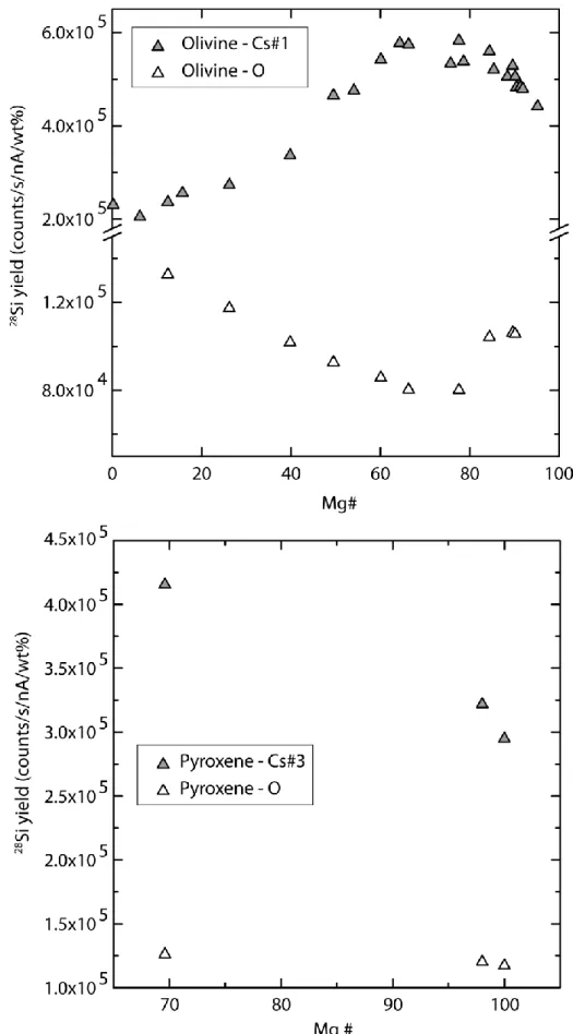
Si ion yields in olivine and low-Ca pyroxene
224
As shown in Fig. 2 and Tables 2 and 3, Si ion yields were clearly different between the different 225
matrices studied (olivine, low-Ca pyroxene, and quartz) and the two primary ion sources used (one 226
session using the RF source and three using the Cs source, producing positive and negative secondary 227
ions, respectively). Indeed, Si ion yields with the Cs source were ~1.5 times better than with the O 228
source for quartz, ~2.5–4 times better for low-Ca pyroxene, and ~2–7 times better for olivine 229
standards (Fig. 2, Tables 2, 3). The Si ion yield evolves differently depending on the primary ion 230
source; the 28Si+ yield is stable with Mg# whereas the 28Si– yield slightly decreases in low-Ca pyroxene 231
(Fig. 2). Olivine positive and negative ion yields similarly show opposite behaviors (Fig. 2). 232
Clear differences in ion yields between different matrices have been previously observed8,35. In 233
olivine, the evolution of the Si ion yield with Mg# is not linear; 28Si– yields increase until Mg# ≈ 70–75, 234
then decrease, whereas 28Si+ yields decrease until the same SiO2 content and then increase (Fig. 2). 235
The same systematic for 28Si+ was previously observed by Steele et al.35 who indicated a minimum 236
near Mg# = 65 (they did not investigate 28Si–). Chaussidon et al.7 showed a similar systematic for the 237
Mg ion yield in olivine with a change in behavior also at Mg# = 75. These complex changes of Si (and 238
Mg) ion yields that affect both polarities are puzzling, since olivine is a solid solution with nothing 239
particular in its chemical and structural properties at Mg# ≈ 70–75. Since olivines have relatively 240
restricted Si atomic contents, these changes must be in some way related to changes in their Fe and 241
Mg contents, and therefore related to the ionic bonding between Si and Mg/Fe in the olivine 242
structure. A kind of ‘competition’ between elements for ionization, which would enhance or suppress 243
the emissivity of a specific element depending on its atomic environment during sputtering, has been 244
previously proposed to explain some complex ionization behaviors8,9. Thus, Chaussidon et al.7 245
proposed an empirical model based on the difference in enthalpies of atomization between Fe and 246
Mg (used as a proxy for bond strength difference between Fe and Mg) that successfully fit Mg ion 247
yields and IMF in olivine standards and CMAS and basaltic glasses. They showed that Mg ion yields 248
and IMFs can be modeled with a two-component ionization including (i) a simple ionization process 249
correlated with the Mg content and (ii) an enhanced ionization process amplified by the presence of 250
Fe. A similar approach might be possible for Si ion yields in olivine, but the problem is more complex 251
since Si ionization relies on the variations and interactions of both Mg and Fe. Therefore, we did not 252
find a satisfactory way to model the evolution of the Si ion yield in olivine. 253
In low-Ca pyroxene, variations of ion yields are limited for Mg# between 70 and 100 for both 28Si+ and 254
28
Si- (Fig. 2). Such behavior is consistent with Steele et al. study35. 255
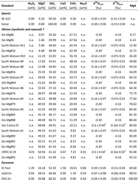
IMF of Si isotopes in olivine and low-Ca pyroxene
256
To our knowledge, no systematic study of Si isotopic analyses in olivine and low-Ca pyroxene by SIMS 257
has been reported in the literature. IMF variations in olivine as a function of Mg# are shown in Fig. 3 258
(complete data are available in Tables 1–3). Obviously, IMF in olivine strongly relies on the 259
abundances of FeO and MgO. In secondary positive polarity, δ29Siinstr decreases non-linearly by ~3‰ 260
over the range Mg# ≈ 10–70, then increases linearly by ~6‰ up to Mg# = 95 (Fig. 3). In secondary 261
negative polarity, δ29Siinstr value increases nonlinearly by ~15‰ from Mg# ≈ 0 until reaching a plateau 262
at Mg# ≈ 70 (Fig. 3). IMF with the RF source can be fitted with a polynomial regression over the range 263
Mg# ≈ 10–70 and then a linear regression yielding residual of 0.16‰, whereas IMF with the Cs source 264
can be fitted with a polynomial function yielding a residual of 0.22‰ (and even better over Mg# = 265
70–95; Fig. 3, Table 4). IMF with the Cs source is very well constrained above Mg# = 45 and is thus 266
useful for IMF corrections in high-MgO olivines. In contrast, it may be preferable to analyze high-FeO 267
olivines with the RF source, although the Si ion yield is lower. In any case, as with Mg and O isotopic 268
measurements in olivine7,17, a comprehensive set of standards is needed to avoid artificial isotopic 269
fractionations and to ensure high precision IMF corrections for Si isotopes. 270
IMF in low-Ca pyroxene shows very small and linear variations with Mg# from 70-100 (Fig. 3). In 271
secondary positive polarity, δ29Siinstr value decreases linearly by ~0.1‰ whereas it increases linearly 272
by ~0.15‰ in secondary negative polarity (Fig. 2). Therefore, IMF can be fitted with linear 273
regressions yielding a residual of 0.01 for both sources. 274
Conclusions
275
Ion yields and IMFs in olivine show complex behaviors that rely on variations in both MgO and FeO 276
content (Fig. 2, 3). In secondary negative polarity, IMF is well constrained above Mg# = 45, and 277
particularly in the range Mg# = 70–100 where δ29Siinstr value does not vary. Therefore, these settings 278
are appropriate for high-accuracy Si isotopic analyses of high-MgO olivines. In contrast, δ29Siinstr value 279
does not vary much over Mg# = 0–70 in positive polarity; such settings are thus appropriate for 280
analyses of high-FeO olivine. Ion yields and IMFs in low-Ca pyroxene are more predictable as they 281
show limited variations over Mg# = 70-100. 282
Acknowledgment: This work was supported by PNP-INSU (French national program of planetology)
283
and ANR CASSYSS (ANR-18-CE31-0010-01, PI J.V.). This is CRPG publication #2705. 284
References
285
1. Moynier F, Vance D, Fujii T, Savage PS. The Isotope Geochemistry of Zinc and Copper. Rev 286
Mineral Geochemistry. 2017;82(1):543-600. doi:10.2138/rmg.2017.82.13
287
2. Dauphas N, John SG, Rouxel OJ. Iron Isotope Systematics. Rev Mineral Geochemistry. 288
2017;82(1):415-510. doi:10.2138/rmg.2017.82.11 289
3. Poitrasson F. Silicon Isotope Geochemistry. Rev Mineral Geochemistry. 2017;82:289-344. 290
doi:10.2138/rmg.2017.82.8 291
4. Villeneuve J, Chaussidon M, Libourel G. Homogeneous Distribution of 26Al in the Solar System 292
from the Mg Isotopic Composition of Chondrules. Science (80- ). 2009;325(5943):985-988. 293
doi:10.1126/science.1173907 294
5. Kita NT, Huberty JM, Kozdon R, Beard BL, Valley JW. High-precision SIMS oxygen, sulfur and 295
iron stable isotope analyses of geological materials: Accuracy, surface topography and crystal 296
orientation. Surf Interface Anal. 2011;43(1-2):427-431. doi:10.1002/sia.3424 297
6. Marin-Carbonne J, Chaussidon M, Boiron MC, Robert F. A combined in situ oxygen, silicon 298
isotopic and fluid inclusion study of a chert sample from Onverwacht Group (3.35Ga, South 299
Africa): New constraints on fluid circulation. Chem Geol. 2011;286(3-4):59-71. 300
doi:10.1016/j.chemgeo.2011.02.025 301
7. Chaussidon M, Deng Z, Villeneuve J, et al. In Situ Analysis of Non-Traditional Isotopes by SIMS 302
and LA–MC–ICP–MS: Key Aspects and the Example of Mg Isotopes in Olivines and Silicate 303
Glasses. Rev Mineral Geochemistry. 2017;82(1):127-163. doi:10.2138/rmg.2017.82.5 304
8. Shimizu N, Hart S. R. Applications of the ion microprobe to geochemistry and 305
cosmochemistry. Annu Rev Earth Planet Sci. 1982;10:483-526. 306
9. Benninghoven A, Rudenauer FG, Werner HW. Secondary Ion Mass Spectrometry: Basic 307
Concepts, Instrumental Aspects, Applications and Trends. United States: John Wiley and
308
Sons,New York, NY; 1987. http://www.osti.gov/scitech/servlets/purl/6092161. 309
10. Reed SJB. Ion microprobe analysis a review of geological applications. Mineral Mag. 310
1989;53:3-24. 311
11. Hinton RW. Ion microprobe trace-element analysis of silicates: Measurement of multi-312
element glasses. Chem Geol. 1990;83(1-2):11-25. doi:10.1016/0009-2541(90)90136-U 313
12. Eiler JM, Graham C, Valley JW. SIMS analysis of oxygen isotopes : matrix effects in complex 314
minerals and glasses. Chem Geol. 1997;138:221-244. 315
13. Deloule E, France-Lanord C, Albarede F. D/H analysis of minerals by ion probe. Geochem Soc 316
Spec Publ. 1991;3:53-62.
317
14. Deloule E, Chaussidon M, Allé P. Instrumental limitations for isotope measurements with a 318
Caméca® ims-3f ion microprobe: Example of H, B, S and Sr. Chem Geol Isot Geosci Sect. 319
1992;101(1-2):187-192. 320
15. Chaussidon M, Albarède F. Secular boron isotope variations in the continental crust: an ion 321
microprobe study. Earth Planet Sci Lett. 1992;108(4):229-241. 322
16. Chaussidon M, Libourel G, Krot AN. Oxygen isotopic constraints on the origin of magnesian 323
chondrules and on the gaseous reservoirs in the early Solar System. Geochim Cosmochim 324
Acta. 2008;72(7):1924-1938. doi:10.1016/j.gca.2008.01.015
325
17. Isa J, Kohl IE, Liu MC, Wasson JT, Young ED, McKeegan KD. Quantification of oxygen isotope 326
SIMS matrix effects in olivine samples: Correlation with sputter rate. Chem Geol. 2017;458:14-327
21. doi:10.1016/j.chemgeo.2017.03.020 328
18. Hartley ME, Thordarson T, Taylor C, Fitton JG, EIMF. Evaluation of the effects of composition 329
on instrumental mass fractionation during SIMS oxygen isotope analyses of glasses. Chem 330
Geol. 2012;334:312-323. doi:10.1016/J.CHEMGEO.2012.10.027
331
19. Rollion-Bard C, Marin-Carbonne J. Determination of SIMS matrix effects on oxygen isotopic 332
compositions in carbonates. J Anal At Spectrom. 2011;26(6):1285. doi:10.1039/c0ja00213e 333
20. Śliwiński MG, Kitajima K, Kozdon R, et al. Secondary Ion Mass Spectrometry Bias on Isotope 334
Ratios in Dolomite–Ankerite, Part I: δ18O Matrix Effects. Geostand Geoanalytical Res. 335
2016;40(2):157-172. doi:10.1111/j.1751-908X.2015.00364.x 336
21. Tissandier L, Rollion-Bard C. Influence of glass composition on secondary ion mass 337
spectrometry instrumental mass fractionation for Si and Ca isotopic analyses. Rapid Commun 338
Mass Spectrom. 2017;31(4):351-361. doi:10.1002/rcm.7799
339
22. De Bievre P, Taylor PDP. Table of the isotopic compositions of the elements. Int J Mass 340
Spectrom Ion Process. 1993;123(2):149-166.
341
23. Ringwood AE. Silicon in the metal phase of enstatite chondrites and some geochemical 342
implications. Geochim Cosmochim Acta. 1961;25(1):1-13. 343
24. Keil K. Mineralogical and chemical relationships among enstatite chondrites. J Geophys Res. 344
1968;73(22):6945-6976. 345
25. Piani L, Marrocchi Y, Libourel G, Tissandier L. Magmatic sulfides in the porphyritic chondrules 346
of EH enstatite chondrites. Geochim Cosmochim Acta. 2016;195:84-99. 347
doi:10.1016/j.gca.2016.09.010 348
26. Zinner E, Ming T, Anders E. Large isotopic anomalies of Si, C, N and noble gases in interstellar 349
silicon carbide from the Murray meteorite. Nature. 1987;330:730-732. 350
27. Basile-Doelsch I, Meunier JD, Parron C. Another continental pool in the terrestrial silicon cycle. 351
Nature. 2005;433(7024):399-402. doi:10.1038/nature03217
352
28. Knight KB, Kita NT, Mendybaev RA, Richter FM, Davis AM, Valley JW. Silicon isotopic 353
fractionation of CAI-like vacuum evaporation residues. Geochim Cosmochim Acta. 354
2009;73(20):6390-6401. doi:10.1016/j.gca.2009.07.008 355
29. Heck PR, Huberty JM, Kita NT, Ushikubo T, Kozdon R, Valley JW. SIMS analyses of silicon and 356
oxygen isotope ratios for quartz from Archean and Paleoproterozoic banded iron formations. 357
Geochim Cosmochim Acta. 2011;75(20):5879-5891.
358
30. Marin-Carbonne J, Chaussidon M, Robert F. Micrometer-scale chemical and isotopic criteria 359
(O and Si) on the origin and history of Precambrian cherts: Implications for paleo-temperature 360
reconstructions. Geochim Cosmochim Acta. 2012;92(March):129-147. 361
doi:10.1016/j.gca.2012.05.040 362
31. Marin-Carbonne J, Robert F, Chaussidon M. The silicon and oxygen isotope compositions of 363
Precambrian cherts: A record of oceanic paleo-temperatures? Precambrian Res. 364
2014;247:223-234. doi:10.1016/j.precamres.2014.03.016 365
32. Valkiers S, Ruße K, Taylor P, Ding T, Inkret M. Silicon isotope amount ratios and molar masses 366
for two silicon isotope reference materials: IRMM-018a and NBS28. Int J Mass Spectrom. 367
2005;242(2-3):321-323. doi:10.1016/j.ijms.2004.11.027 368
33. Sio CKI, Dauphas N, Teng F-Z, Chaussidon M, Helz RT, Roskosz M. Discerning crystal growth 369
from diffusion profiles in zoned olivine by in situ Mg-Fe isotopic analyses. Geochim 370
Cosmochim Acta. 2013;123:302-321. doi:10.1016/j.gca.2013.06.008
371
34. Armytage RMG, Georg RB, Savage PS, Williams HM, Halliday AN. Silicon isotopes in meteorites 372
and planetary core formation. Geochim Cosmochim Acta. 2011;75(13):3662-3676. 373
doi:10.1016/j.gca.2011.03.044 374
35. Steele IM, Hervig RL, Hutcheon ID, Smith J V. Ion microprobe techniques and analyses of 375
olivine and low-Ca pyroxene. Am Mineral. 1981;66(5-6):526-546. 376
377
Figures captions
378
Fig. 1: Stability of NL615 and Sonar quartz standards over the different analytical sessions (see tables 379
2 and 3). Dashed lines and grey boxes correspond to average values and external reproducibilities (2σ 380
standard deviation) respectively. 381
382 383
Fig. 2: 28Si ion yields in both polarities as a function of Mg# in olivine (top) and in low-Ca pyroxene 384
(bottom). 385
Fig. 3: δ29Sinorm value as a function of Mg# in olivine (top) and in low-Ca pyroxene (bottom). The 387
polynomial function regression is calculated from the olivine data of session #1 with the Cs source 388
(δ29Sinorm = -10.19 - 0.09×Mg# + (1.38×10⁻²)×Mg#2 - (1.79×10⁻⁴)×Mg#3 + (6.57×10⁻⁷)×Mg#4). Data for 389
olivine with the RF source are fitted with a polynomial function for Mg# < 65 (δ29Sinorm = -10.98 + 390
0.02×Mg# - (8.69×10⁻⁴)×Mg#2) and a linear function for Mg# > 65 (δ29Sinorm = -30.60 + 0.25×Mg#). 391
Data for low-Ca pyroxene are fitted with linear functions for both polarities, i.e. δ29Sinorm = 5.95 + 392
(4.90×10⁻³)×Mg# with the Cs source and δ29Sinorm = -6.87 + (3.95×10⁻³)×Mg# with the RF source. 393
394 395 396
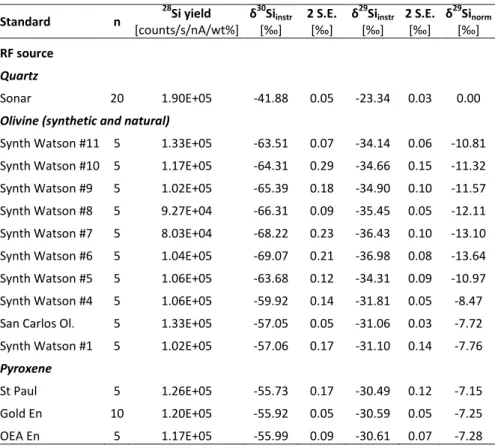
Table 1: Chemical compositions, bulk Si isotopic compositions normalized to NBS 28 (errors are 2 S.E., 397
when available), Mg numbers of the studied standards. See text for details and parameter 398
definitions. Isotopic compositions in italic are estimated (see text for details) 399 Standard Al2O3 [wt%] MgO [wt%] SiO2 [wt%] CaO [wt%] FeOT [wt%] Na2O [wt%] δ30Sitrue [‰] δ29Sitrue [‰] Mg# Quartz NL 615 0.00 0.10 99.50 0.00 0.50 n.a. -0.30 ± 0.03 -0.15 ± 0.03 n.a.
Sonar 0.00 0.00 100.00 0.00 0.00 n.a. -0.38 ± 0.06 -0.21± 0.04 n.a.
Olivine (synthetic and natural) †
Sio-Mg#0 n.a. 0.07 29.26 n.a. 67.21 n.a. -0.30 -0.16 0.17
Sio-Mg#6 n.a. 2.46 29.99 n.a. 67.56 n.a. -0.30 -0.16 6.14
Synth Watson #11 n.a. 5.06 30.60 n.a. 64.34 n.a. -0.16 ± 0.07 -0.07± 0.01 12.40
Sio-Mg#16 n.a. 6.48 30.94 n.a. 62.58 n.a. -0.30 -0.16 15.71
Synth Watson #10 n.a. 11.19 32.05 n.a. 56.76 n.a. -0.16 ± 0.07 -0.07± 0.01 26.20 Synth Watson #9 n.a. 17.83 33.61 n.a. 48.56 n.a. -0.16 ± 0.07 -0.07± 0.01 39.80 Synth Watson #8 n.a. 22.98 34.82 n.a. 42.20 n.a. -0.16 ± 0.07 -0.07± 0.01 49.50
Sio-Mg#54 n.a. 25.55 35.42 n.a. 39.03 n.a. -0.30 -0.16 54.09
Synth Watson #7 n.a. 29.05 36.25 n.a. 34.71 n.a. -0.16 ± 0.07 -0.07± 0.01 60.10
SiO-Mg#64 n.a. 31.61 36.85 n.a. 31.54 n.a. -0.30 -0.16 64.34
Synth Watson #6 n.a. 32.83 37.14 n.a. 30.04 n.a. -0.16 ± 0.07 -0.07± 0.01 66.30
Sio-Mg#76 n.a. 38.97 38.58 n.a. 22.45 n.a. -0.30 -0.16 75.75
Synth Watson #5 n.a. 40.22 38.88 n.a. 20.90 n.a. -0.16 ± 0.07 -0.07± 0.01 77.60
Sio-Mg#79 n.a. 40.93 39.04 n.a. 20.03 n.a. -0.30 -0.16 78.62
Synth Watson #4 n.a. 45.02 40.00 n.a. 14.98 n.a. -0.16 ± 0.07 -0.07± 0.01 84.40
Sio-Mg#85 n.a. 45.74 40.17 n.a. 14.09 n.a. -0.30 -0.16 85.39
Sio-Mg#88 n.a. 48.00 40.71 n.a. 11.29 n.a. -0.30 -0.16 88.44
San Carlos Ol n.a. 48.88 40.91 n.a. 10.21 n.a. -0.3 ± 0.04¤ -0.16± 0.02¤ 89.60 Synth Watson #1 n.a. 49.33 41.02 n.a. 9.65 n.a. -0.16 ± 0.07 -0.07± 0.01 90.20
Sio-Mg#90 n.a. 49.55 41.07 n.a. 9.37 n.a. -0.30 -0.16 90.49
Sio-Mg#91 n.a. 50.21 41.23 n.a. 8.57 n.a. -0.30 -0.16 91.34
Sio-Mg#92 n.a. 50.63 41.33 n.a. 8.04 n.a. -0.30 -0.16 91.89
CRPG SC Ol 0.03 50.94 41.32 0.07 7.21 0.01 -0.3 ± 0.04¤ -0.16± 0.02¤ 92.68
Sio-Mg#95 n.a. 53.25 41.94 n.a. 4.81 n.a. -0.30 -0.16 95.22
Pyroxene
St Paul 1.39 24.18 52.30 1.58 19.01 0.06 -0.49 ± 0.05 -0.21± 0.04 69.60
Gold En 0.93 38.52 58.46 0.09 1.39 0.03 -0.07 ± 0.08 -0.06± 0.04 98.03
OEA En 0.04 39.88 60.62 0.00 0.00 0.04 -0.04 ± 0.04 -0.02± 0.04 100.00
†Chemical composition data from 7,33. ¤ Data from 34
400 401
Table 2: Number of analyses (n), 28Si yield, raw isotopic data, and IMFs normalized to NBS28 from 402
MC-SIMS analyses with the RF source (positive secondary polarity) 403 Standard n 28 Si yield [counts/s/nA/wt%] δ30Siinstr [‰] 2 S.E. [‰] δ29Siinstr [‰] 2 S.E. [‰] δ29Sinorm [‰] RF source Quartz Sonar 20 1.90E+05 -41.88 0.05 -23.34 0.03 0.00
Olivine (synthetic and natural)
Synth Watson #11 5 1.33E+05 -63.51 0.07 -34.14 0.06 -10.81
Synth Watson #10 5 1.17E+05 -64.31 0.29 -34.66 0.15 -11.32
Synth Watson #9 5 1.02E+05 -65.39 0.18 -34.90 0.10 -11.57
Synth Watson #8 5 9.27E+04 -66.31 0.09 -35.45 0.05 -12.11
Synth Watson #7 5 8.03E+04 -68.22 0.23 -36.43 0.10 -13.10
Synth Watson #6 5 1.04E+05 -69.07 0.21 -36.98 0.08 -13.64
Synth Watson #5 5 1.06E+05 -63.68 0.12 -34.31 0.09 -10.97
Synth Watson #4 5 1.06E+05 -59.92 0.14 -31.81 0.05 -8.47
San Carlos Ol. 5 1.33E+05 -57.05 0.05 -31.06 0.03 -7.72
Synth Watson #1 5 1.02E+05 -57.06 0.17 -31.10 0.14 -7.76
Pyroxene St Paul 5 1.26E+05 -55.73 0.17 -30.49 0.12 -7.15 Gold En 10 1.20E+05 -55.92 0.05 -30.59 0.05 -7.25 OEA En 5 1.17E+05 -55.99 0.09 -30.61 0.07 -7.28 404 405
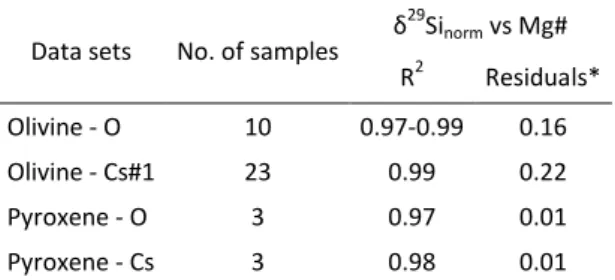
Table 3: Number of analyses (n), 28Si yield, raw isotopic data, and IMFs IMFs normalized to NBS28 406
from MC-SIMS analyses with the Cs source (negative secondary polarity). 407 Standard Session n 28 Si yield [counts/s/nA/wt%] δ29Siinstr [‰] 2 S.E. [‰] δ29Siinstr [‰] 2 S.E. [‰] δ29Sinorm [‰] Cs source Quartz NL615 #1 25 2.49E+05 -28.96 0.05 -14.45 0.04 0.00 NL615 #2 10 3.16E+05 -28.89 0.06 -14.45 0.03 0.00 Sonar #3 10 2.18E+05 -29.68 0.11 -15.77 0.09 0.00
Olivine (synthetic and natural)
Sio-Mg#0 #1 5 2.31E+05 -48.47 0.30 -24.63 0.33 -10.19
Sio-Mg#6 #1 5 2.05E+05 -49.54 0.43 -25.16 0.27 -10.71
Synth Watson #11 #1 5 2.37E+05 -47.32 0.50 -23.87 0.49 -9.42
Sio-Mg#16 #1 5 2.56E+05 -44.24 0.40 -22.32 0.22 -7.88
Synth Watson #10 #1 5 2.73E+05 -41.67 0.18 -20.93 0.11 -6.48
Synth Watson #9 #1 5 3.36E+05 -33.34 0.25 -16.80 0.15 -2.36
Synth Watson #8 #1 5 4.65E+05 -25.08 0.21 -12.57 0.12 1.88
Sio-Mg#54 #1 5 4.75E+05 -22.52 0.42 -11.29 0.26 3.16
Synth Watson #7 #1 5 5.42E+05 -20.59 0.18 -10.30 0.13 4.15
SiO-Mg#64 #1 5 5.77E+05 -18.97 0.20 -9.41 0.09 5.03
Synth Watson #6 #1 5 5.75E+05 -18.28 0.16 -9.14 0.10 5.31
Sio-Mg#76 #1 5 5.33E+05 -17.14 0.17 -8.52 0.10 5.93
Synth Watson #5 #1 5 5.83E+05 -16.31 0.17 -8.02 0.13 6.43
Sio-Mg#79 #1 5 5.37E+05 -16.54 0.14 -8.16 0.04 6.28
Synth Watson #4 #1 5 5.59E+05 -15.58 0.26 -7.79 0.17 6.66
Sio-Mg#85 #1 5 5.20E+05 -16.44 0.26 -8.05 0.10 6.40
Sio-Mg#88 #1 5 5.05E+05 -16.20 0.19 -7.96 0.06 6.49
San Carlos Ol #1 5 5.29E+05 -15.67 0.17 -7.72 0.15 6.73
Synth Watson #1 #1 5 5.05E+05 -16.15 0.21 -7.96 0.12 6.49
Sio-Mg#90 #1 5 4.83E+05 -16.15 0.19 -7.98 0.16 6.46
Sio-Mg#91 #1 5 4.84E+05 -16.35 0.16 -8.01 0.07 6.44
Sio-Mg#92 #1 5 4.79E+05 -16.25 0.26 -7.98 0.16 6.46
Sio-Mg#95 #1 5 4.41E+05 -16.44 0.18 -8.03 0.17 6.42
Synth Watson #11 #2 5 2.84E+05 -47.06 0.22 -23.90 0.16 -9.46
Synth Watson #10 #2 5 3.19E+05 -42.41 0.55 -21.41 0.53 -6.96
Synth Watson #8 #2 5 5.35E+05 -23.70 0.24 -11.83 0.17 2.61
Synth Watson #6 #2 5 6.56E+05 -17.02 0.14 -8.35 0.13 6.10
Synth Watson #4 #2 5 6.49E+05 -14.36 0.12 -7.00 0.06 7.45
Synth Watson #1 #2 5 5.84E+05 -14.83 0.17 -7.31 0.10 7.14
CRPG SC Ol #2 10 6.65E+05 -14.56 0.10 -7.12 0.03 7.33 pyroxene St Paul #3 5 4.16E+05 -17.30 0.11 -9.48 0.08 6.29 Gold En #3 5 3.22E+05 -17.01 0.16 -9.33 0.16 6.44 OEA En #3 5 2.95E+05 -17.06 0.22 -9.32 0.08 6.43 408
Table 4: Coefficients of determination and average residuals of IMF (δ29Sinorm) as a function of Mg# 409
for the different sessions and standard sets. 410
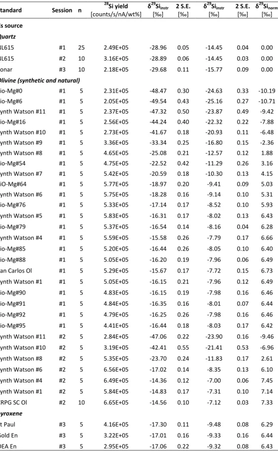
Data sets No. of samples δ
29 Sinorm vs Mg# R2 Residuals* Olivine - O 10 0.97-0.99 0.16 Olivine - Cs#1 23 0.99 0.22 Pyroxene - O 3 0.97 0.01 Pyroxene - Cs 3 0.98 0.01
* Residuals are expressed in ‰ and are calculated as: residual = (Σ| δ29Sinorm - δ29Sicalc |)/(no. analyses), with δ29Sinorm the 411
isotopic ratio measured for one sample and δ29Sicalc the isotopic ratio of the same sample calculated from the regression 412
curves.
413 414