HAL Id: cea-03175313
https://hal-cea.archives-ouvertes.fr/cea-03175313
Submitted on 19 Mar 2021
HAL is a multi-disciplinary open access
archive for the deposit and dissemination of
sci-entific research documents, whether they are
pub-lished or not. The documents may come from
teaching and research institutions in France or
abroad, or from public or private research centers.
L’archive ouverte pluridisciplinaire HAL, est
destinée au dépôt et à la diffusion de documents
scientifiques de niveau recherche, publiés ou non,
émanant des établissements d’enseignement et de
recherche français ou étrangers, des laboratoires
publics ou privés.
ROOSTER: a machine-learning analysis tool for Kepler
stellar rotation periods
S. N. Breton, A. R. G. Santos, L. Bugnet, S. Mathur, R. A. García, P. L. Pallé
To cite this version:
S. N. Breton, A. R. G. Santos, L. Bugnet, S. Mathur, R. A. García, et al.. ROOSTER: a
machine-learning analysis tool for Kepler stellar rotation periods. Astronomy and Astrophysics - A&A, EDP
Sciences, 2021, 647, pp.A125. �10.1051/0004-6361/202039947�. �cea-03175313�
A&A 647, A125 (2021) https://doi.org/10.1051/0004-6361/202039947 c S. N. Breton et al. 2021
Astronomy
&
Astrophysics
ROOSTER: a machine-learning analysis tool for Kepler stellar
rotation periods
S. N. Breton
1, A. R. G. Santos
2, L. Bugnet
1, S. Mathur
3,4, R. A. García
1, and P. L. Pallé
3,41 AIM, CEA, CNRS, Université Paris-Saclay, Université Paris Diderot, Sorbonne Paris Cité, 91191 Gif-sur-Yvette, France
e-mail: [email protected]
2 Space Science Institute, 4765 Walnut Street, Suite B, Boulder, CO 80301, USA 3 Instituto de Astrofísica de Canarias, 38200 La Laguna, Tenerife, Spain
4 Universidad de La Laguna, Dpto. de Astrofísica, 38205 La Laguna, Tenerife, Spain
Received 20 November 2020/ Accepted 25 January 2021
ABSTRACT
In order to understand stellar evolution, it is crucial to efficiently determine stellar surface rotation periods. Indeed, while they are of great importance in stellar models, angular momentum transport processes inside stars are still poorly understood today. Surface rotation, which is linked to the age of the star, is one of the constraints needed to improve the way those processes are modelled. Statistics of the surface rotation periods for a large sample of stars of different spectral types are thus necessary. An efficient tool to automatically determine reliable rotation periods is needed when dealing with large samples of stellar photometric datasets. The objective of this work is to develop such a tool. For this purpose, machine learning classifiers constitute relevant bases to build our new methodology. Random forest learning abilities are exploited to automate the extraction of rotation periods in Kepler light curves. Rotation periods and complementary parameters are obtained via three different methods: a wavelet analysis, the autocorrelation function of the light curve, and the composite spectrum. We trained three different classifiers: one to detect if rotational modulations are present in the light curve, one to flag close binary or classical pulsators candidates that can bias our rotation period determination, and finally one classifier to provide the final rotation period. We tested our machine learning pipeline on 23 431 stars of the Kepler K and M dwarf reference rotation catalogue for which 60% of the stars have been visually inspected. For the sample of 21 707 stars where all the input parameters are provided to the algorithm, 94.2% of them are correctly classified (as rotating or not). Among the stars that have a rotation period in the reference catalogue, the machine learning provides a period that agrees within 10% of the reference value for 95.3% of the stars. Moreover, the yield of correct rotation periods is raised to 99.5% after visually inspecting 25.2% of the stars. Over the two main analysis steps, rotation classification and period selection, the pipeline yields a global agreement with the reference values of 92.1% and 96.9% before and after visual inspection. Random forest classifiers are efficient tools to determine reliable rotation periods in large samples of stars. The methodology presented here could be easily adapted to extract surface rotation periods for stars with different spectral types or observed by other instruments such as K2, TESS or by PLATO in the near future.
Key words. methods: data analysis – stars: solar-type – stars: activity – stars: rotation – starspots
1. Introduction
Low-mass stars with convective outer layers (hereafter solar-type stars) can exhibit magnetic activity (e.g.,Brun & Browning 2017). In the Sun, one of the manifestations of magnetic activity is the emergence of magnetic spots at its surface. While for stars other than the Sun, one cannot directly image starspots in great detail, one can in principle detect their impact on, for example, stellar brightness. As the star rotates, starspots come in and out of the visible hemisphere, thus modulating the stellar brightness. As a consequence, such spot modulation encloses information on stellar magnetic activity and surface rotation (e.g.,Berdyugina 2005;Strassmeier 2009).
Surface rotation periods represent a key parameter to under-stand stellar angular momentum transport. This process is not yet sufficiently understood in order to be correctly implemented in stellar evolution codes (e.g., Aerts et al. 2019, and refer-ences therein). Neglecting angular momentum transport may have a significant impact on the stellar age estimates (e.g.,
Eggenberger et al. 2010). These stellar ages are crucial for study-ing the evolution of the Milky Way (e.g., Miglio et al. 2013), as well as for a better characterisation of planetary systems (e.g., Huber 2018). The evolution of planetary systems, which is driven by tidal and magnetic effects, is indeed strongly influ-enced by the stellar rotation rate, through angular
momen-tum exchange between planets and their host star star (e.g.,
Zhang & Penev 2014; Mathis 2015; Bolmont & Mathis 2016;
Strugarek et al. 2017;Benbakoura et al. 2019).
The surface rotation period is found to be a strong func-tion of the stellar age: low-mass stars with an external convec-tive envelope spin down during their main-sequence evolution. The first empirical relation between the two stellar parameters was proposed bySkumanich(1972, also known as Skumanich spin-down law). In particular, for young main-sequence solar-type stars, the rotation period can be used to constrain stellar ages through the so-called gyrochronology relations (e.g.,Barnes 2003,2007;Mamajek & Hillenbrand 2008;Meibom et al. 2011,
2015; García et al. 2014a). However, for stars older than the Sun, the ages determined by gyrochronology deviate from the asteroseismic ages (Angus et al. 2015; van Saders et al. 2016).
Angus et al.(2020) also show that the empirical gyrochronology relations cannot reproduce the stellar ages inferred from veloc-ity dispersion. These discrepancies justify the need for improved gyrochronology relations. Furthermore, the presence of surface rotational modulation in the light curves has a limiting effect on the detection of low-amplitude transiting exoplanets (e.g.,
Cameron 2017). The amplitude of those rotational modulations is directly linked to the surface stellar magnetic activity level and leads to difficulties in performing asteroseismic analysis of active solar-like stars because this magnetism inhibits pulsations
Open Access article,published by EDP Sciences, under the terms of the Creative Commons Attribution License (https://creativecommons.org/licenses/by/4.0),
(e.g., García & Ballot 2019;Mathur et al. 2019, and references therein).
During its four-year nominal mission, the Kepler satel-lite (Borucki et al. 2010) collected high-quality, long-term, and nearly continuous photometric data for almost 200 000 targets (Mathur et al. 2017) in the Cygnus-Lyra region. After the fail-ure of two reaction wheels, Kepler was reborn as a new mis-sion called K2 (Howell et al. 2014). K2 observed more than 300 000 targets around the ecliptic (Huber et al. 2016) over 20 three-month campaigns. The Transiting Exoplanet Survey Satel-lite (TESS,Ricker et al. 2015) observed nearly the all sky dur-ing its nominal mission. TESS gathered data for tens of millions of stars with an observational length ranging from 27 days to one year. This large amount of observations represent the best photometric dataset to study the distribution of stellar surface rotation periods, Prot. But to reach this goal and extract periods
for large samples of stars, automatic procedures are required. Such an attempt was recently undertaken with a deep learning approach using convolutional neural networks (Blancato et al. 2020). However, training those networks requires a heavy com-putational power. Hence, the development of an easy-to-train machine learning procedure coupled with the outputs of widely-used rotation pipelines will be an extremely valuable asset. Indeed, this is the objective of the current study.
Random forest (RF) algorithms (Breiman 2001) are either able to classify large samples of stars (when used for classifica-tion) or to provide parameter estimates (when used for regres-sion). In asteroseismology, RF algorithms have already been used to estimate stellar surface gravities (log g, Bugnet et al. 2018) and to automatically recognise solar-like pulsators (Bugnet et al. 2019). They have also recently been used to per-form analyses linked to surface stellar rotation, but only in order to infer long rotation periods from TESS 27-day-long light curves (Lu et al. 2020). In this work, we present the Random fOrest Over STEllar Rotation (ROOSTER), which is designed to select a rotation period for stars observed by Kepler through a combination of RF classifiers applied to a variety of methods used to extract Protand different ways to correct the light curves.
Thus, the main goal of ROOSTER is to automatically achieve a large degree of reliability that could even be improved by per-forming a small number of human visual validation of certain results, which are also suggested by the pipeline.
The layout of the paper is as follows. Section 2 presents the sample of K and M stars used in this work as well as the methodology to extract the surface rotation periods. Section3
describes all the parameters used to feed ROOSTER. In Sect.4, we explain how the ROOSTER pipeline is built and we detail the training scheme we chose for this work. In Sect. 5, we present the rotation periods obtained with the ROOSTER pipeline and the strategy implemented for stars with missing input parame-ters. Results, limitations, and possibilities to increase the accu-racy of ROOSTER are discussed in Sect.6. Finally, conclusions and perspectives are given in Sect.7.
2. Observations and methodology to extract surface rotation periods
The target sample of this work is comprised of main-sequence K and M stars observed by the Kepler mission. This sample was the one analysed in the rotation study done bySantos et al.
(2019). It is the most complete rotation catalogue for the Kepler K and M dwarfs. Hereafter, this catalogue is referred asS19. In it, 26 521 targets were selected according to the Kepler Stellar Properties Catalogue for Data Release 25 (DR25,Mathur et al.
2017) and for 15 290 of them, a Protwas provided. As the
pur-pose of this work is rotation analysis, different types of poten-tial contaminants are removed from our study, namely Kepler objects of interest, eclipsing binaries, misclassified red giants, misclassified RR Lyrae, light curves with photometric pollution by nearby stars or multiple signals, classical pulsators (namely δ Scuti and/or γ Doradus) candidates, and contact binary candi-dates (seeS19for details on the contaminants).
S19determined average rotation periods, Prot, and average
pho-tometric activity indexes (Sph,Mathur et al. 2014), for more than
60% of the targets. In fact, about 30% of the reported ProtbyS19
are new detections in comparison with the previous largest Prot
catalogue (McQuillan et al. 2014). In addition to an automatic selection of reliable Prot, theS19analysis required an extensive
amount of visual examinations (see Sect.2.2), which justifies the need for a pipeline such as ROOSTER.
2.1. Light curve preparation
We use three sets of KEPSEISMIC light curves1, the same used in S19. KEPSEISMIC data is calibrated using KADACS (Kepler Asteroseimic Data Analysis and Calibration Software;
García et al. 2011), which applies customised apertures and cor-rects for outliers, jumps, drifts, and discontinuities at the edges of the Kepler Quarters. Because regular interruptions in the obser-vations (such as the gaps induced every three days due to the angular momentum dump of the Kepler satellite) could produce a false detection of Prot, gaps shorter than 20 days are filled by
implementing inpainting techniques using a multi-scale discrete cosine transform (García et al. 2014b;Pires et al. 2015).
We use in particular three different data sets obtained with three high-pass filters, with cutoff periods at 20, 55, and 80 days. The transfer function is unity for periods shorter than the cut-off period, while for longer periods it varies sinusoidaly, slowly approaching zero at twice the cutoff period. Thus, for a given filter, it is possible to recover periods longer than the respective cutoff period. The main goal of using and comparing three differ-ent filters is to find the best trade-off between filtering the unde-sired instrumental modulations at long periods while keeping the intrinsic stellar rotational signal. KEPSEISMIC light curves are optimised for asteroseismic studies, but are also very well suited for rotation and magnetic activity studies (see for exam-ple Appendix B inS19).
2.2. Methodology to extract Prot
Surface rotation periods can be studied with different meth-ods, namely: periodogram analysis (e.g.,Reinhold et al. 2013;
Nielsen et al. 2013); Gaussian processes (e.g., Angus et al. 2018); gradient power spectrum analysis (e.g., Shapiro et al. 2020; Amazo-Gómez et al. 2020); autocorrelation function (ACF, e.g.,McQuillan et al. 2013, 2014); time-period analysis based on wavelets (e.g.,Mathur et al. 2010;García et al. 2014a); or with a combination of different diagnostics such as the com-posite spectrum (CS, e.g.,Ceillier et al. 2016,2017;Santos et al. 2019). Using artificial data,Aigrain et al. (2015) compared the performance of different pipelines used to determine the rotation. The authors found that the combination of the data set prepa-ration and different rotation diagnostics, in particular the one implemented in this work (see next paragraph), yields the best set of results in terms of reliability and completeness.
1 KEPSEISMIC data are available at MAST via http://dx.doi.
In this work, we use the procedure followed inS19to extract Prot combining three analysis methods (time-period analysis,
ACF, and CS) with the KEPSEISMIC light curves. Those Prot
are respectively denoted PACF, PGWPSand PCS. Control
param-eters related to the ACF and CS are also extracted, they are denoted HACF, GACF, and HCS. Each method also allows us to
compute a magnetic activity proxy Sph. Description and details
concerning those parameters can be found in AppendixA. During the visual examination inS19, a group of classical pulsators (CP) and close binaries (CB) candidates was identified. Those stars are referred hereafter as Type 1 CP/CB candidates. These targets are typically fast rotators (Prot< 7 days), showing
very stable and fast beating patterns, a large number of harmon-ics in the power spectrum, and/or very large Sphvalues.
Interest-ingly,Simonian et al.(2019) found that the majority of the fast rotators observed by Kepler are tidally-synchronised binaries. In fact, there is a significant overlap between the Type 1 CP/CB candidates and the tidally-synchronised binaries (seeS19). This suggests that the modulation seen in the light curve of such objects may still be related to rotation but not of single targets. Therefore, we advice caution while studying such targets. In
S19, the Type 1 CP/CB candidates were flagged through visual inspection.
3. Parameters used to feed the machine learning algorithms
To ensure that ROOSTER is able to identify targets with detectable rotation modulation and to extract reliable rotation periods, the selection of relevant parameters is crucial. They will help the algorithm to perform successive classifications as described in Sect.4. Indeed, a random forest algorithm relies on the following principle: during the training step, a forest of clas-sification trees is grown to perform splits between the elements with different labels (Breiman 2001). From the root of the tree, the training sample is progressively separated in purer (consider-ing the labels) sub-samples. This task is performed by select(consider-ing at each iteration the best split over a range of randomly generated range of splits using the input parameters.
The three rotation periods (PACF, PGWPS, and PCS) obtained
thanks to the method described in Sect.2.2and in AppendixA, combined with the three sets of data corresponding to the three different high-pass filtered KEPSEISMIC light curves (20, 55 and 80 days), yield a total of 9 rotation-period candidates for each star. The objective is to train the algorithm to choose the rotation period given inS19. To do so, we also feed our pipeline with the parameters (amplitude, central value and standard devi-ation) of the five first Gaussian functions fitted on the GWPS and the CS. If, for a given star, the ith Gaussian function could not be fitted, the corresponding parameters are set to zero. We also include the χ2of the two fits, the number of Gaussian functions fitted to each GWPS and CS and the mean level of noise. This makes 108 additional input parameters (36 for each filter). As only a few stars have a sixth Gaussian function fitted for both GWPS and CS method, we verified that keeping the correspond-ing parameters out of the classification does not affect the result. We also feed the random forest algorithm with the HACF, GACF,
and HCSfor each filter, and the Sphwith corresponding errors for
each method and each filter, leading to 27 more parameters. Because the rotation periods depend on the global parame-ters of the stars (age, spectral type, etc.), we complement our set of input parameters with the effective temperature, Teff, and
logarithm of surface gravity log g from the DR25 catalogue (Mathur et al. 2017). We also decide to use the Flicker in Power
metric (FliPer,Bugnet et al. 2018), which is correlated with the stellar surface gravity. FliPer is a measure of the total power in the stellar power spectral density (PSD) between a low frequency cut-off, νCand the Nyquist frequency, νN. It can be defined as:
FliPer (νC)= 1 νN−νC Z νN νC PSD(ν) dν − Pn, (1)
where Pnis an estimate of the photon noise level which depends
on the magnitude of the star. In this work, we used a noise esti-mation calibrated with the whole set of KEPSEISMIC calibrated light curves. We consider the following four FliPer values: F0.7,
F7, F20, F50for νCof 0.7, 7, 20 and 50 µHz, respectively.
Additional parameters linked to the quality of the stellar tar-gets and of the acquired light curves are added: Kepler mag-nitude values Kp from the Kepler input catalogue (Brown et al. 2011), length of the light curves (in days), bad quarter flag, num-ber of bad quarters in the light curve, and finally, the start time and end time of the light curve.
For each star, a total of 159 input parameters are used to feed the ROOSTER pipeline. The full list of parameters is given in TableB.1.
4. The ROOSTER pipeline
ROOSTER uses three random forest classifiers2: RotClass, which selects stars that have a rotation signal; PollFlag, which flags the Type-1 CP/CB candidates; and PeriodSel, which allows ROOSTER to choose the final rotation period between the three different filters and the three analysis methods. Due to its ability to take into account a large number of parameters, its flexibility, and its adaptability to the training set, the random forest algo-rithm constitutes a clear improvement from the former method consisting in defining thresholds on a small number of key parameters.
The three classifiers are trained with the same 159 input parameters per star as defined in the previous section, but each classifier considers different training sets and gives different out-put labels. Depending on the task the classifier has to achieve, each of them may give different importance to the input param-eters. The flow diagram of ROOSTER is shown in Fig.1. 4.1. Description
The first ROOSTER classifier, RotClass, separates stars with rota-tional modulations (labelled Rot stars) from other stars (labelled NoRotstars). These NoRot stars are rejected and are no longer considered in the rest of the analysis (although some of those stars may later still be flagged for visual checks). An example of Rot star, KIC 1164583, is presented in Fig.2. In this figure, the light curves and the output of the three different rotation period retrieval methods (WPS/GWPS, ACF, and CS) are shown.
In general, the risk of confusion by the ROOSTER pipeline between a Rot and a NoRot star is a consequence of two main issues: it can be difficult to reliably detect low-amplitude rota-tional modulations and Kepler instrumental effects may intro-duce additional periodic modulations in the light curve.
A small fraction of Rot stars (generally stars with Prot < 7
days) may be close-in binaries or classical pulsator stars can-didates. As mentioned above, the detected signal for this type of targets may not be consistent with rotation of single stars. The PollFlag classifier is trained to identify these CP/CP candi-dates and flag them as FlagPoll, while the rest of the stars are
2 The random forests classifiers are implemented with the Python
Fig. 1.Structure of the ROOSTER pipeline. The yellow diamonds out-line the action of each classifier used by the machine learning algo-rithm. The stars of the sample (lightblue parallelogram) are anlaysed by the pipeline. The red and dark blue parallelograms emphasis the label attributed by the ROOSTER classifiers to each star of the sample. First, stars with rotational modulation are selected by RotClass and the label Rotor NoRot is given. NoRot stars are not considered in the subse-quent analysis. The PollFlag classifier flags Type 1 CP/CB candidates (labelled FlagPoll). The remainder of the stars receive the FlagOk label. Finally, the PeriodSel classifier selects the rotation period.
labelled FlagOk. The light curve and PSD of the FlagPoll can-didate, KIC 2283703, is shown as an example in Fig.3. Its Type 1 CP/CB character can be recognised due to the large amplitude of the brightness variations, the beating pattern, and the large number of high-amplitude peaks in the PSD.
Finally, the third classifier, PeriodSel, is trained with the same 159 parameters defined in Sect. 2. This time, the labels of the training set correspond to the nine possible rotation peri-ods (PACF, PCS, PGWPS in the 20, 55, and 80-day filters). The
goal is to select the most reliable period among those nine esti-mates, which may differ. For example, Fig. 2 illustrates the impact of the high-pass filter when producing the light curves of KIC 1164583. The 55- and 80-day filters indicate a 47-day period, while the period detected from the 20-day filter is 21 days. The comparison between the three WPS shows that the 47-day signal has been filtered out by the 20-day filter. The WPS shows power at longer periods which is another evidence for a
longer period being filtered. The 47-day GWPS period of the 55-day filter is finally chosen as the retrieved Prot. PeriodSel selects
one of the nine estimates as the retrieved rotation period, Prot,ML.
We emphasise that the transfer function of a given filter slowly approaches zero at twice the cutoff period, that is to say it is pos-sible to retrieve rotation periods longer than the cutoff period of the filter applied to the light curve.
4.2. Training
The followed approach allows us to show the robustness of ROOSTER. In particular, ROOSTER must be weakly dependent to the exact composition of the training set. This can be only achieved if the training-set parameter space distribution is simi-lar to the test-set parameter space distribution. Hence, we decide to perform a training-loop process where the three classifiers are trained one hundred times. Each time, the full working sample is randomly divided in a training set (containing 75% of the stars) and a test set (containing 25% of the stars). The number of times each star is drawn in the test set over the one hundred training repetitions follows a binomial law with probability p= 0.25 and number of trials n= 100.
In total, the target sample of this study includes 23 431 tar-gets fromS19: 21 707 of them have all the parameters from the rotation pipeline (referred as the RotClass sample), while 1,724 have missing parameters (referred as the MissingParam sample, mainly due to missing ACF values).S19gives measured Protfor
14 936 stars: 14 562 for the RotClass sample and 374 stars for the MissingParamsample. These stars are labelled Rot and are then used with the PeriodSel classifier (called the PeriodSel sample). A total of 8495 stars do not have a reliable ProtinS19. Hence,
thisS19sample is ideal to train and evaluate the performance of ROOSTER. The MissingParam sample is not considered at this stage but will be used later in Sect.5.2. The working PollFlag sample is constituted of 630 stars: 315 Type 1 CP/CB candidates completed at each training with 315 other stars randomly cho-sen from the PeriodSel sample. The composition of the different samples is summarised in Table1.
An RF classifier not only gives a label to each classified star, its forest structure also allows obtaining the proportion of trees attributing a given class to each considered star. Indeed, the final classification of the target corresponds to the label that is selected by the majority of the trees. We can then define the classification ratio as the number of trees giving the output label over the total number of trees of the forest. This ratio is useful to estimate the reliability of the machine-learning output for each star.
Since we perform a training loop with random repetitions, we are also able to compute the mean classification ratio for each star. This mean classification ratio is computed as the mean of all the classification ratios found each time a star has been drawn in the test set.
5. Results
In what follows, the accuracy term is defined as the agreement of any label given by a ROOSTER classifier and theS19catalogue taken as a reference.
From the 21 707 stars of the RotClass sample, the mean clas-sification ratio gives the right label (Rot or NoRot) for 20 443 stars, which yields an overall accuracy of ∼94.2%. We find that 1707 stars have been misclassified at least once during the 100 runs (7.9%) while 1259 stars have been misclassified in half of the repetitions of the training they were part of the test set (5.8%). Finally, 884 stars have been systematically misclassified
20-da y filter 55-da y filter 80-da y filter a) b) c) d) Fig . 2. Comparison between the light curv es obtained with the three high pass filters for KIC 1164583 (fr om left to right , 20, 55, and 80-day filter respecti v ely). (a ) KEPSEISMIC light curv e. (b ) W av elet po wer spectrum (left) and global w av elet po wer spectrum (right). The grid represents the cone of influence of the reliable periodicity . High-amplitude po wer are highlighted by black and red whereas green and blue denote lo w-amplitude po wer . (c ) Auto-Correlation Function. (d ) Composite spectrum (black) and corresponding best fit with multiple Gaussian profiles (green). In all panels, the dashed line sho ws the position of the extracted rotation period.
0 200 400 600 800 1000 1200 1400 Time (days) 4 2 0 2 4 Fl ux (x 10 4 ppm ) 102 101 100 101 102 Frequency ( Hz) 108 106 104 102 100 102 PS D (p pm 2/Hz )
Fig. 3.PSD of the Type 1 CP/CB candidate KIC 2283703. The light
curve is characterised by high-amplitude flux variation and beating patterns over time, while the PSD exhibits a large number of high-amplitude peaks.
(4.1%). The accuracy of RotClass is already valuable but can be improved with a limited amount of visual checks. By performing visual inspections, we verify that the highest number of misclas-sifications occur within the mean classification ratio between 0.4 and 0.8. For this reason, stars within these mean classification ratios should be part of the visual verification for future target samples. In the case of the target sample of the current study, 2230 stars (10.3%) are within this interval. One of the reasons for the misclassifications is the presence of instrumental modu-lations that can be mistaken by rotation periods.
Concerning PollFlag, the goal is to obtain a high sensitiv-ity to real Type-1 CP/CB candidates, while keeping the frac-tion of misclassificafrac-tions low. The sensitivity is here defined as the fraction of Type 1 CP/CB candidates correctly identified by PollFlag. Thus, the sensitivity does not take into account the fraction of non-Type 1 CP/CB candidates correctly iden-tified. In this case, it is a more relevant estimator than the accuracy, as the fraction of Type-1 CP/CB candidates in the sample is small. During the training loop, approximately 2.8% of the considered non-Type-1 CP/CB candidates have been misclassified by PollFlag as Type-1 CP/CB candidates. If PollFlaghad been applied blindly on the full PeriodSel sample, this means that approximately 400 non-Type-1 CP/CB candi-dates would have been wrongly flagged. However, considering the mean classification ratio, only two Type-1 CP/CB candi-dates have been misclassified, which yields a PollFlag sensitiv-ity of ∼99.4%. Looking at the detailed results during the training loop, 6 Type-1 CP/CB candidates are misclassified at least once (1.9%), 4 are misclassified in half of the repetitions (1.3%), and none is systematically misclassified.
Finally, the mean classification ratio of the PeriodSel clas-sifier gives us an accuracy of ∼86.8%, that is to say the label corresponding to the rotation period from S19 is attributed to 12 638 stars over 14 562 in the PeriodSel. Nevertheless, a signif-icant fraction of the labels chosen by PeriodSel contains a Prot
which is within 10% of the one inS19. For this reason, we adopt the agreement within 10% as the true accuracy, TA, of PeriodSel in the following way:
TA=Card (Egood)
Card (E) × 100, (2)
with E being the considered ensemble of stars and Egood the
subsample from E where PeriodSel retrieves a Prot,MLmatching
Prot,S19within 10%.
We find that PeriodSel selected an incorrect period for 830 stars at least once (5.7%), for 693 (4.8%) in half of the realisa-tions and systematically for 569 (3.9%). In terms of the mean classification ratio, a correct rotation period Prot,MLis retrieved
for 13 871 stars. Hence, the true accuracy is ∼95.3%. Figure4
shows the comparison between Prot,MLand the reference values
fromS19. From the 1924 stars for which the label attributed by ROOSTER was not the same as in S19, 1233 are within the shaded blue area of the figure. For the remaining 4.7% of the stars, we observe three cases:
1. Among the periods retrieved by ROOSTER, 103 of them lie within a tolerance threshold that is slightly over 10% (see the shaded green area of Fig.4). This could be due to a precision difference between PGWPS, PACF, and PCSor to the filter that was
selected to choose the value of the rotation period.
2. The machine learning mistakes instrumental modulations for real rotation signals when such signatures appear in the light curves. These instrumental modulations usually have periods between 38 and 50 days. 99 ROOSTER rotation periods lie both in this [38–50] days regions and outside of the 10% agreement region.
3. Depending on the rotation signature, some of the nine period estimates correspond to the second harmonic of the cor-rect rotation period. PeriodSel privileges this harmonic over the fundamental period for 381 stars of the PeriodSel sample. 5.1. Weight of the considered parameters
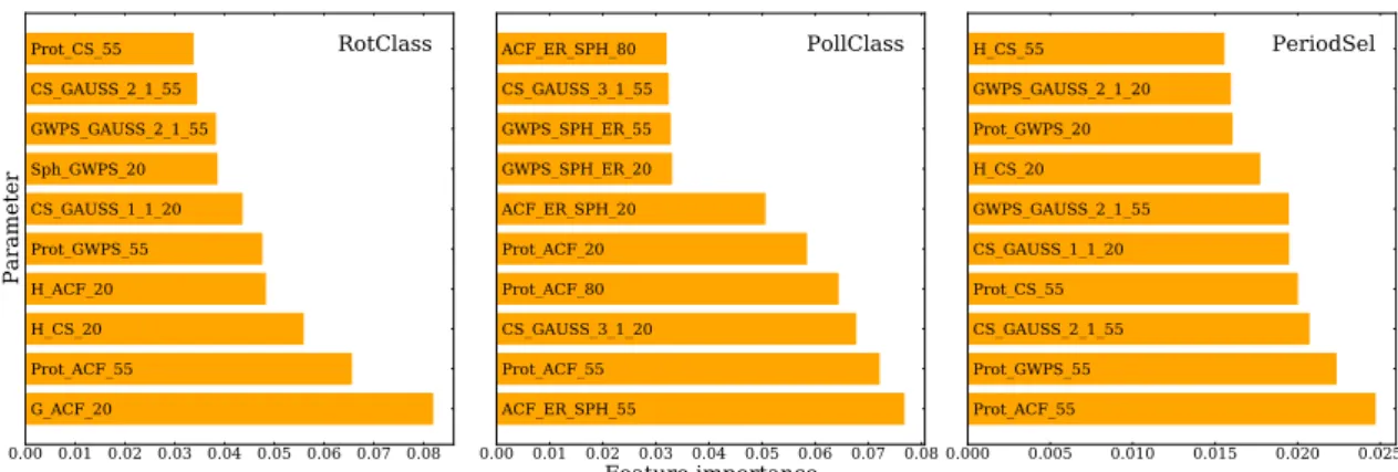
Here we discuss briefly the importance given by the three classi-fiers to the input parameters. For each classifier, Fig.5presents the weights of the ten most important parameters. The rotation periods provided by the ACF and GWPS for the 55-day filter are in the top five parameters of RotClass. PollFlag favours the ACF parameters, which is coherent as the ACF shows a spe-cific pattern for CP/CB candidates. We note that PollFlag is the only classifier among the three that also prioritises errors on Sph
determination to perform the classification. For PeriodSel, three of the most important parameters are the rotation period values computed from the 55-day filtered light curves. The parameters of the Gaussian functions fitted to the GWPS and CS also have a strong influence over the classification. The remainder of the most important parameters are the HACF, GACF, and HCS from
the 20-day filtered light curves, which highlights the importance of those control parameters when considering the reliability of a potential rotation signal.
Finally, one could be concerned by the effect of systematic errors on Teff and log g parameters. However, because of the
small weight of these two parameters, their influence on our classifiers’ accuracy is marginal. Therefore, the impact on our methodology of any systematic error in both parameters is neg-ligible. A similar conclusion will be reached in Sect.6.2where we tested our algorithm using simulated data byAigrain et al.
(2015).
5.2. Strategy for stars with missing parameters
The rotation pipeline does not always provide a value for all the parameters needed for the random forest classification. The majority of the missing parameters are related to the ACF for the 55- and 80-day filters. In general this happens because there is no clear peak in the ACF. However, to perform the classification, an
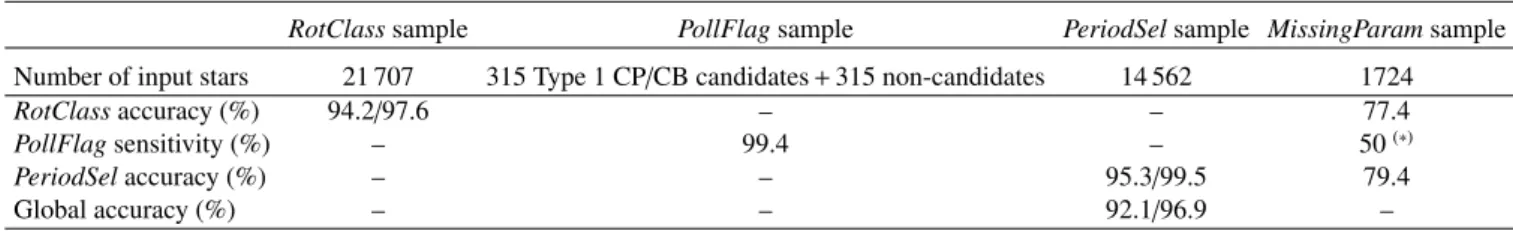
Table 1. Composition of the different subsamples used for the study and scores of the different classifiers.
RotClasssample PollFlagsample PeriodSelsample MissingParam sample Number of input stars 21 707 315 Type 1 CP/CB candidates + 315 non-candidates 14 562 1724
RotClassaccuracy (%) 94.2/97.6 – – 77.4
PollFlagsensitivity (%) – 99.4 – 50(∗)
PeriodSelaccuracy (%) – – 95.3/99.5 79.4
Global accuracy (%) – – 92.1/96.9 –
Notes. The 315 non-candidate stars used in the PollFlag sample are randomly chosen in the PeriodSel sample at each training. For RotClass and PeriodSel, the metrics chosen to express the score is the accuracy while it is the sensitivity for PollFlag. When two scores are given, the first and the second one corresponds to the score before and after visual inspection, respectively.(∗)There is only 4 Type-1 CP/CB candidates in this sample,
among which, only 2 have been correctly classified yielding 50% probability.
input value must be provided for each of the 159 parameters. To test ROOSTER on the stars with missing parameters, we choose to train our three classifiers without the values for PACF, Sph,ACF
and the respective uncertainty for the three filters. However, we decide to keep HACFand GACFas input parameters. If for a given
star in a given filter, PACF is not determined, HACF and GACF
will be set to zero. This is logical in the sense that the value for GACFand HACFindicates whether the corresponding peak is
significant.
Like before, RotClass is trained with the RotClass sample. Only 1334 of the stars of the MissingParam sample are cor-rectly classified (accuracy of 77.4% compared to the accuracy of 94.2% reached with the RotClass sample). This is not a sur-prise in the sense that when the ACF does not yield a period estimate, it suggests that the modulation in the light curve may not be clear enough. This assumption is confirmed when com-paring the fraction of stars with rotation signal in the RotClass sample and in the MissingParam sample: 67.1% of the stars in the RotClass sample are labelled Rot inS19while only 24% of the MissingParam sample are labelled Rot inS19. Thus, the two distributions are very different and this impacts the outcomes of the classifier.
The accuracy loss is similar for PeriodSel, with only 79.4% of rotation period retrieved within 10%. Among the Missing-Param sample, there are only four Type 1 CP/CP candidates, which make it difficult to estimate the sensitivity for this sample. Two of those candidates are correctly flagged (50%).
In order to optimise the efficiency of the pipeline, it is thus preferable to be able to compute upstream a full set of parameters for a maximal number of stars and to avoid having to deal with a too large MissingParam sample.
6. Discussion
The RF classification with ROOSTER represents a clear improvement compared to the automatic selection method based on control parameters performed inS19(see AppendixA). How-ever, for a small fraction of the sample, the ROOSTER results differ from those inS19. Nevertheless, the discrepancies repre-sent well-known issues that we try to flag.
Once we have obtained the rotation periods from the ROOSTER pipeline, we define a list of criteria so that we can flag stars that require visual checks and hence improve the accu-racy of the final retrieval of extracted rotation periods.
1. First, we identify stars for which the proper filter is not selected. We expect Prot,MLchosen by PeriodSel to be coherent
with the filter from which they were extracted. This means that, for Prot,ML < 23 days, Prot,ML should have been extracted from
the 20-day filtered light curve, for 23 days < Prot,ML < 60 days
0 20 40 60 80 100 120 Prot, S19 (days) 0 20 40 60 80 100 120 Prot,M L (d ay s) 500 1000 1500 2000 2500 Number of stars
Fig. 4.Comparison between Prot,MLand the values given inS19for the
stars of the PeriodSel sample. The shaded blue and green areas highlight the 10 and 30% agreement regions, respectively. The number of stars inside this area is colour coded. The stars outside the shaded area are represented by red dots. The dashed blue line corresponds 2:1 line.
from the 55-day filtered light curve, for Prot,ML > 60 days from
the 80-day filtered light curve. If Prot,MLagrees within 15% with
the PGWPS of the proper filter, we replace Prot,MLby this value.
Otherwise, the star is flagged for visual check. This change is motivated by the goal of retrieving the most accurate Sph, which
is generally obtained considering a light curve with a high-pass filter coherent with Prot,ML.
2. As shown in Fig.4, a significant number of stars lie on the 1:2 line, highlighting an issue with the harmonics of Prot, which
can partially be overcome. We flag targets for visual inspection if at least one of the other Protestimates (nine in total) is within
15% of the double of Prot,ML. We notice that this harmonics issue
is generally linked to Protyielded by the GWPS fitting method
that selects a higher-order harmonic instead of the first one as it is more often done by the ACF methodology. In order to reduce the impact of this problem, it would be necessary to perform a comprehensive study of the fitted GWPS harmonic’s pattern. This analysis is out of the scope of the current paper but will be the issue of a future upgrade of the ROOSTER pipeline.
3. The ROOSTER pipeline might also attribute the wrong rotation period because of instrumental modulation in Kepler data. The 55 and 80 day filtered light curves are the most affected by instrumental modulations. For these cases, Prot,ML is
usu-ally between 38 and 50 days, but can be longer. Those instru-mental modulations can be identified through visual inspection of the light curves and of the control figures of the rotation code. For this reason, we flag all stars with Prot,ML > 38 days.
0.00 0.01 0.02 0.03 0.04 0.05 0.06 0.07 0.08 G_ACF_20 Prot_ACF_55 H_CS_20 H_ACF_20 Prot_GWPS_55 CS_GAUSS_1_1_20 Sph_GWPS_20 GWPS_GAUSS_2_1_55 CS_GAUSS_2_1_55 Prot_CS_55 Parameter RotClass 0.00 0.01 0.02 0.03 0.04 0.05 0.06 0.07 0.08 Feature importance ACF_ER_SPH_55 Prot_ACF_55 CS_GAUSS_3_1_20 Prot_ACF_80 Prot_ACF_20 ACF_ER_SPH_20 GWPS_SPH_ER_20 GWPS_SPH_ER_55 CS_GAUSS_3_1_55 ACF_ER_SPH_80 PollClass 0.000 0.005 0.010 0.015 0.020 0.025 Prot_ACF_55 Prot_GWPS_55 CS_GAUSS_2_1_55 Prot_CS_55 CS_GAUSS_1_1_20 GWPS_GAUSS_2_1_55 H_CS_20 Prot_GWPS_20 GWPS_GAUSS_2_1_20 H_CS_55 PeriodSel
Fig. 5.Importance of the ten most important parameters for the three classifiers of the pipeline. The full list of ROOSTER input parameters is given in AppendixB.
Instrumental modulations can correspond to, for example: sud-den bursts in flux; abnormal flux variations which only happen every four Kepler Quarters, that is to say every Kepler year; and flux variations that are present throughout the light curve with a main periodicity of one Kepler year, while in the rotation diag-nostics used here one can identify its harmonics and the result-ing filtered signals. We note that the 80-day filtered KEPSEIS-MIC light curves are naturally the most affected by instrumental modulations. However, the signature in the 20-day and 55-day filtered light curves may also have an instrumental origin. This is also true for other data products in the literature. Avoiding instrumental modulations is one of our objectives and one of the reasons to use three KEPSEISMIC light curves (Sect.2.1) and perform complementary visual checks (see also discussion inS19).
4. Stars with Prot,ML< 1.6 days are also flagged to ensure that
the detected signal is not CP/CB-like. Observationally, synchro-nised binaries correspond to targets with detected period shorter than seven days (Simonian et al. 2019).
5. All the Type 1 CP/CB candidates inS19 have a period shorter than seven days. We therefore flag for visual inspection Type-1 CP/CB candidates detected by PollFlag when Prot,ML> 7
days.
6. Stars for which the length of data or the presence of gaps might not be enough to cover the range of rotation peri-ods expected for the studied stars are also visually inspected. The flagging criterion can be based on the total length of obser-vations (given in days or quarters) and on the continuity of the light curve. In this work we have used a criterion in quar-ters. Stars were flagged if their light curve was shorter than five quarters.
7. The last group of visual checks correspond to stars are those for which the mean classification ration of RotClass is between 0.4 and 0.8, as already stated in Sect.5.
The different types of stars flagged for visual inspection are summarised in Fig.6.
The six conditions listed above result in flagging for visual inspection 4606 stars (31.6% of the PeriodSel sample). Among those 4606 stars, 628 will be corrected after the visual inspec-tion. Finally, for 27 stars, we prefer the value given by the machine learning over theS19value. After this step, we obtain a 99.5% accuracy for the retrieval of Prot,ML. It should be noted
that among the 63 remaining stars outside the 10% agreement between ROOSTER and S19, 24 of them lie in a large toler-ance zone of 30% of the good rotation period. As mentioned in Sect.5, stars with mean classification ratio between 0.4 and 0.8 are visually checked. That means that some of the stars classified
NoRotby RotClass are also visually checked. The total number of visual checks to perform in the scheme we just described is then 5,461 (25.2% of the RotClass sample), which represent a significant improvement compared toS19(60% of the sample was visually checked).
We are able to compute a global accuracy score for both RotClassand PeriodSel classifiers. Among the 14 562 stars of the PeriodSel sample, both RotClass and PeriodSel made correct predictions for 13,413 stars (92.1 % of the sample), that is to say RotClasscorrectly labelled them Rot and Prot,MLagrees within
10% of the Protgiven inS19. After the visual checks, this
accu-racy is raised to 96.9%. The accuaccu-racy scores before and after visual inspection are summarised in Table1.
We note that it could be possible to reduce the global amount of visual checks. For example, 683 stars are flagged only because their light curve was shorter than five quarters. It represents 4.7% of the PeriodSel sample. Among those 683 stars, only 7 of them are actually corrected after the visual inspection. The visual check of short light curves could therefore be avoided without a significant loss of accuracy. However, concerning the methodol-ogy described in this paper, we decided to clearly point out every risk of confusion that could occur in ROOSTER.
6.1. Period retrieval in short light curves
The ROOSTER accuracy on short light curves may yield inter-esting hints about the performance of our method on a dataset constituted by stars observed by TESS or K2. Our dataset contains 29 light curves with length within 30 and 35 days and 690 light curves with length within 35 and 150 days. Period-Sel accuracy over those two subsamples is 96.5% and 92.9%, respectively. The Prot distribution for those two subsamples is
presented in Fig.7. All the stars with light curves length below 35 days present rotation periods below five days. The ability of our method to retrieve longer Protin such short light curves is
beyond the scope of this paper and will be discussed in details in a subsequent study.
6.2. Period retrieval with simulated data
ROOSTER was also applied on the simulated data of the hare and hounds exercise inAigrain et al.(2015). The results of this analysis are presented in AppendixC. For the purpose of this exercise, ROOSTER was trained considering only light curves from S19 and had no previous knowledge of the simulated data. We found that ROOSTER applied blindly performed better than any of the methods compared inAigrain et al.(2015). The
0
20
40
60
80
100
120
P
rot, S19(days)
0
20
40
60
80
100
120
P
rot,M L(d
ay
s)
Harmonic flag
Long trend flag (P
rot, ML38 days)
Filter flag
Stars flagged CP/CB1 with P
rot, ML7 days
Short trend flag (P
rot, ML1.6 days)
Short lightcurves ( 4 quarters)
Fig. 6. Comparison between the ML
retrieved period and the value given in
S19. The 10% tolerance region is rep-resented in blue, while the large toler-ance zone (30%) is shown in green. Stars that are flagged for visual checks are highlighted: yellow circle show the stars selected with the filter condition, red dia-monds those by the long trend condi-tion, cyan triangle those selected by har-monic search condition, brown stars those selected with the short light curve con-dition, green cross those selected by the short trend condition, and orange cross the stars flagged as Type 1 CP/CB with Prot,ML> 7 days. 0 10 20 30 40 50 60 Prot, S19 (days) 0 20 40 60 80 100 120 140 160 Number of stars 0 1 2 3 4 5 Prot, S19 (days) 0 5 10 15
Fig. 7.Left: Protdistribution for stars with light curves within 35 and 150 days. Right: same as left panel, but for stars with light curves within 30
and 35 days.
ROOSTER accuracy scores are close to what we obtain on real data in this study. It is important to notice that in this analysis Teff
and log g were not used in the training in order to have the same homogeneous set of parameters for the noise-free and noisy light curves.
7. Conclusion
In this paper, we have described ROOSTER, a machine learn-ing analysis pipeline dedicated to obtain rotation periods with a small amount of visual verification. ROOSTER has been suc-cessfully applied to targets observed by the Kepler main mission.
The pipeline is built around three random forest classifiers, each one in charge of a dedicated task: detecting rotational modula-tions, flagging close binary and classical pulsator candidates, and selecting the correct rotation period, respectively with the clas-sifiers RotClass, PollFlag and PeriodSel.
We applied ROOSTER to the K and M main-sequence dwarfs analysed in S19 (Santos et al. 2019). We were able to detect rotation periods with an accuracy of 94.2% for a ple of 21 707 stars (RotClass sample). Within the RotClass sam-ple, we considered 14,562 stars with measured rotation periods (PeriodSel sample). The automatic analysis yields a true accu-racy of 95.3% for PeriodSel, that is to say an agreement of the
rotation period from ROOSTER within 10% of the reference value fromS19. We noticed that the majority of the misclassi-fied stars were due to known effects, in particular, instrumen-tal modulations and confusion with a harmonic of the true rota-tion period. 31.6% of the stars of the PeriodSel sample are then flagged for visual checks which allows us to correct wrong val-ues for 628 more stars and raises the PeriodSel accuracy to 99.5%. Considering the results of the combined RotClass and PeriodSelsteps on the PeriodSel sample, the global accuracy of ROOSTER is estimated at 92.1% without any visual check, and 96.9% after visual inspection of 25.2 % of the RotClass sample (against 60% inS19). By removing some input parameters from the ROOSTER training, we were also able to deal with stars with missing input parameters, at the price of a loss of accuracy. How-ever, this accuracy loss is not only due to the diminution of the number of the parameters, but is also related to the intrinsic qual-ity of the light curves for which the rotation pipeline was not able to provide a full set of parameters.
It should be emphasised that the accuracy estimated here is only valid for the K and M dwarf stars studied inS19. Rotation signals for hotter stars (mid F to G) are more complex than for K and M. In order to extend our analysis to those stars, a signifi-cant sample of hotter stars should first be introduced in the train-ing set. The different accuracy values should also be reassessed before proceeding to the analysis. The length of the Kepler time series and the exquisite quality of the photometric measurements are important advantages for rotational analyses. To analyse light curves from K2 or TESS (which have a typical observational length significantly shorter than those of Kepler), first we need to verify whether the current training set is appropriate. If this is not the case, the classifiers must be trained with more suit-able training sets (e.g by building a new training set with K2 or TESS stars). The selection of targets for visual inspection would probably be modified too.
Nevertheless, the global framework of ROOSTER can be adapted the Kepler F and G main-sequence solar type stars (Santos et al., in prep.). It should also be possible to use this technique to analyse data from K2, TESS and, in a near future, PLATO (PLAnetary Transit and Oscillations,Rauer et al. 2014). Such large-scale survey would be a great asset for gyrochronol-ogy models and our understanding of stellar spinning evolution in relation with age and spectral type.
Acknowledgements. We thank Suzanne Aigrain and Joe Llama for pro-viding us with the simulated data used in Aigrain et al. (2015). S. N. B., L. B. and R. A. G. acknowledge the support from PLATO and GOLF CNES grants. A. R. G. S. acknowledges the support from NASA under grant NNX17AF27G. S. M. acknowledges the support from the Spanish Ministry of Science and Innovation with the Ramon y Cajal fellowship number RYC-2015-17697. P. L. P. and S. M. acknowledge support from the Spanish Ministry of Science and Innovation with the grant number PID2019-107187GB-I00. This research has made use of the NASA Exoplanet Archive, which is operated by the California Institute of Technology, under contract with the National Aeronautics and Space Administration under the Exoplanet Exploration Program. Software: Python (Van Rossum & Drake 2009), numpy (Oliphant 2006), pandas (The pandas development team 2020; McKinney 2010), matplotlib (Hunter 2007), scikit-learn (Pedregosa et al. 2011). The source code used to obtain the present results can be found at: https://gitlab.com/sybreton/pushkin;
https://gitlab.com/sybreton/ml_surface_rotation_paper.
References
Aerts, C., Mathis, S., & Rogers, T. M. 2019,ARA&A, 57, 35
Aigrain, S., Llama, J., Ceillier, T., et al. 2015,MNRAS, 450, 3211
Amazo-Gómez, E. M., Shapiro, A. I., Solanki, S. K., et al. 2020,A&A, 636, A69
Angus, R., Aigrain, S., Foreman-Mackey, D., & McQuillan, A. 2015,MNRAS, 450, 1787
Angus, R., Morton, T., Aigrain, S., Foreman-Mackey, D., & Rajpaul, V. 2018,
MNRAS, 474, 2094
Angus, R., Beane, A., Price-Whelan, A. M., et al. 2020,AJ, 160, 90
Barnes, S. A. 2003,ApJ, 586, 464
Barnes, S. A. 2007,ApJ, 669, 1167
Benbakoura, M., Réville, V., Brun, A. S., Le Poncin-Lafitte, C., & Mathis, S. 2019,A&A, 621, A124
Berdyugina, S. V. 2005,Liv. Rev. Sol. Phys., 2, 8
Blancato, K., Ness, M., Huber, D., Lu, Y., & Angus, R. 2020, ApJ, submitted [arXiv:2005.09682]
Bolmont, E., & Mathis, S. 2016,Celest. Mech. Dyn. Astron., 126, 275
Borucki, W. J., Koch, D., Basri, G., et al. 2010,Science, 327, 977
Breiman, L. 2001,Mach. Learn., 45, 5
Brown, T. M., Latham, D. W., Everett, M. E., & Esquerdo, G. A. 2011,AJ, 142, 112
Brun, A. S., & Browning, M. K. 2017,Liv. Rev. Sol. Phys., 14, 4
Bugnet, L., García, R. A., Davies, G. R., et al. 2018,A&A, 620, A38
Bugnet, L., García, R. A., Mathur, S., et al. 2019,A&A, 624, A79
Cameron, A. C. 2017, inThe Impact of Stellar Activity on the Detection and Characterization of Exoplanets, eds. H. J. Deeg, & J. A. Belmonte (Cham: Springer International Publishing), 1
Ceillier, T., van Saders, J., García, R. A., et al. 2016,MNRAS, 456, 119
Ceillier, T., Tayar, J., Mathur, S., et al. 2017,A&A, 605, A111
Domingo, V., Fleck, B., & Poland, A. I. 1995,Sol. Phys., 162, 1
Eggenberger, P., Miglio, A., Montalban, J., et al. 2010,A&A, 509, A72
Fröhlich, C., Romero, J., Roth, H., et al. 1995,Sol. Phys., 162, 101
García, R. A., & Ballot, J. 2019,Liv. Rev. Sol. Phys., 16, 4
García, R. A., Hekker, S., Stello, D., et al. 2011,MNRAS, 414, L6
García, R. A., Ceillier, T., Salabert, D., et al. 2014a,A&A, 572, A34
García, R. A., Mathur, S., Pires, S., et al. 2014b,A&A, 568, A10
Howell, S. B., Sobeck, C., Haas, M., et al. 2014,PASP, 126, 398
Huber, D. 2018, inAsteroseismology and Exoplanets: Listening to the Stars and Searching for New Worlds, eds. T. L. Campante, N. C. Santos, & M. J. P. F. G. Monteiro, 49, 119
Huber, D., Bryson, S. T., Haas, M. R., et al. 2016,ApJS, 224, 2
Hunter, J. D. 2007,Comput. Sci. Eng., 9, 90
Jenkins, J. M., Caldwell, D. A., Chandrasekaran, H., et al. 2010,ApJ, 713, L87
Liu, Y., San Liang, X., & Weisberg, R. H. 2007,J. Atmos. Oceanic Technol., 24, 2093
Lu, Y., Angus, R., Agüeros, M. A., et al. 2020,AJ, 160, 168
Mamajek, E. E., & Hillenbrand, L. A. 2008,ApJ, 687, 1264
Mathis, S. 2015,A&A, 580, L3
Mathur, S., García, R. A., Régulo, C., et al. 2010,A&A, 511, A46
Mathur, S., García, R. A., Ballot, J., et al. 2014,A&A, 562, A124
Mathur, S., Huber, D., Batalha, N. M., et al. 2017,ApJS, 229, 30
Mathur, S., García, R. A., Bugnet, L., et al. 2019,Front. Astron. Space Sci., 6, 46
McKinney, W. 2010, inProceedings of the 9th Python in Science Conference, eds. S. van der Walt, & J. Millman, 56
McQuillan, A., Mazeh, T., & Aigrain, S. 2013,ApJ, 775, L11
McQuillan, A., Mazeh, T., & Aigrain, S. 2014,ApJS, 211, 24
Meibom, S., Barnes, S. A., Latham, D. W., et al. 2011,ApJ, 733, L9
Meibom, S., Barnes, S. A., Platais, I., et al. 2015,Nature, 517, 589
Miglio, A., Chiappini, C., Morel, T., et al. 2013,MNRAS, 429, 423
Nielsen, M. B., Gizon, L., Schunker, H., & Karoff, C. 2013,A&A, 557, L10
Oliphant, T. 2006,NumPy: A guide to NumPy(USA: Trelgol Publishing) The pandas development team 2020, https://github.com/pandas-dev/
pandas/
Pedregosa, F., Varoquaux, G., Gramfort, A., et al. 2011,J. Mach. Learn. Res., 12, 2825
Pires, S., Mathur, S., García, R. A., et al. 2015,A&A, 574, A18
Rauer, H., Catala, C., Aerts, C., et al. 2014,Exp. Astron., 38, 249
Reinhold, T., Reiners, A., & Basri, G. 2013,A&A, 560, A4
Ricker, G. R., Winn, J. N., Vanderspek, R., et al. 2015,J. Astron. Telesc. Instrum. Syst., 1, 014003
Santos, A. R. G., García, R. A., Mathur, S., et al. 2019,ApJS, 244, 21
Shapiro, A. I., Amazo-Gómez, E. M., Krivova, N. A., & Solanki, S. K. 2020,
A&A, 633, A32
Simonian, G. V. A., Pinsonneault, M. H., & Terndrup, D. M. 2019,ApJ, 871, 174
Skumanich, A. 1972,ApJ, 171, 565
Strassmeier, K. G. 2009,A&ARv, 17, 251
Strugarek, A., Bolmont, E., Mathis, S., et al. 2017,ApJ, 847, L16
Torrence, C., & Compo, G. P. 1998,Bull. Am. Meteorol. Soc., 79, 61
Van Rossum, G., & Drake, F. L. 2009,Python 3 Reference Manual(Scotts Valley, CA: CreateSpace)
van Saders, J. L., Ceillier, T., Metcalfe, T. S., et al. 2016,Nature, 529, 181
Appendix A: Detailed parameter extraction methodology
This appendix presents in detail of the methodology used to extract the Protcandidates considered by ROOSTER.
The first method used to measure Protis a time-period
anal-ysis using a wavelet decomposition (Torrence & Compo 1998;
Liu et al. 2007;Mathur et al. 2010). Wavelets of different
peri-ods, each one taken as the convolution between a sinusoidal and a Gaussian function (Morlet wavelet), are cross-correlated with the light curve to obtain the wavelet power spectrum (WPS, see left panel of (b) in Fig.2). The WPS is projected over the period-axis to obtain the one-dimension Global Wavelet Power Spec-trum (GWPS, see right panel of (b) in Fig.2). Multiple Gaussian functions are fitted to the GWPS starting by the one with the highest amplitude. The fitted Gaussian function is removed and the next highest Gaussian peak is fitted in an iterative way until no peaks are above the noise level. Thus, the first period esti-mate, corresponding to the period of the highest fitted peak in the GWPS, is assigned as the rotation period recovered by this methodology: PGWPS. The period uncertainty is taken as the
half width at half maximum (HWHM) of the Gaussian function. Although this is a very conservative approach, it allows us to take into account variations due to differential rotation as part of the uncertainty.
The second analysis method is the ACF of the light curve. The rotation period, PACF, corresponds to the period of the
high-est peak in the ACF at a lag greater than zero. Two other param-eters are computed: GACFand HACF. GACFis the height of PACF,
while HACFis the mean difference between the height of PACF
and the two local minima on both sides of PACF(see an extended
description inCeillier et al. 2017).
The third method is the composite spectrum (CS). CS is the product between the normalized GWPS and ACF. This way, the peaks present in both GWPS and ACF (possibly related to rota-tion) are amplified while the signals appearing only in one of the two methods (for example due to instrumental effects that have a different manifestation in each analysis) are attenuated. Mul-tiple Gaussian functions are fitted to the CS following the same iterative procedure as the one described for the GWPS. PCS is
obtained as the period of the fitted Gaussian of highest ampli-tude and the uncertainty is its HWHM. The ampliampli-tude of this peak is HCS.
Having three period estimates for each light curve (PGWPS,
PACF, and PCS), S19 computed the respective value for the
photometric activity index Sph (that is to say, one for each
Prot estimation). Sph is computed as defined by Mathur et al.
(2014), being the standard deviation over light curve segments of 5 × Prot. The final Sph value we provide corresponds to the
average Sph. Sph is corrected for the photon-shot noise
follow-ingJenkins et al.(2010). For some targets this correction leads to negative Sph values. Most of the targets in this situation do not
show rotational modulation. For those with rotational modula-tion and Sph< 0 (a few percent of the targets),S19applied
indi-vidually a different correction to the photon-shot noise, which is computed from the high-frequency noise component in the power density spectrum. We note that the Sph value has only
a physical sense when rotational modulation is detected in the light curve and, thus, Protis measured (e.g.,Mathur et al. 2014,
Egeland et al., in prep.).
InS19, a first group of stars with reliable rotation periods is automatically selected when there is a good agreement between the different period estimates and the heights for PACF and PCS
are larger than a given threshold (see S19 for details; height thresholds adopted fromCeillier et al. 2017). For the remainder of the targets (about 60%), in order to decide whether the signal is related to rotational modulation and to select the correct Prot, S19visually inspected the respective light curves, rotation diag-nostics, and power spectra. During the visual inspection 40% of the final selected Protwere recovered. There are different
prob-lems causing the measurement of a different Protin each
method-ology. For example: small amplitudes of the rotational modu-lation, which translate into small values of Sph, HACF, GACF,
and HCS; presence of instrumental modulations; and strong
har-monic of Prot. Instrumental modulations affect primarily the light
curves obtained with the 55-day and 80-day filters. However, we note that depending on the Prot value, the correct period may
not be recovered from the 20-day filter. Half of the rotation period can be wrongly retrieved as Prot(what we call strong
har-monic) when the dominant spots producing the rotational signal are apart by ∼180◦in longitude. In our methodology, the GWPS is the most sensitive to this issue, while the ACF is the least sen-sitive. The performance of the ACF in these cases is discussed in detail byMcQuillan et al.(2013,2014). InS19, the decision on the filter used for the final Protrelies on two criteria: preserving
the instrinsic rotational signal with the Sphvalue not affected by
filtering, while minimizing the impact of possible instrumental effects which may not alter the period estimate but may affect Sph. Typically the 20-day filter is selected for Prot ≤ 23 days,
the 55-day filter is selected for 23 < days Prot ≤ 60 days, and
the 80-day filter is selected for Prot > 60 days. For the rotation
period estimate itself the priority is given to PGWPS. The main
reason for this choice is the conservative uncertainty for PGWPS.
Appendix B: Input parameters
The detailed set of 159 parameters used to train Rot-Class, PollFlag and PeriodSel is presented in Table B.1. GWPS_GAUSS_1_i_XX, GWPS_GAUSS_2_i_XX and GWPS_GAUSS_3_i_XX respectively correspond to the ampli-tude, the central period and the standard deviation of the ith
Gaussian fitted in the GWPS with the XX-day filter. The same naming convention has been used for CS_GAUSS_1_i_XX, CS_GAUSS_2_i_XX and CS_GAUSS_3_i_XX with the CS.
Table B.1. 159 input parameters used to train the RF classifiers.
ACF_ER_SPH_20 ACF_ER_SPH_55 ACF_ER_SPH_80 BAD_Q_FLAG CS_CHIQ_20 CS_CHIQ_55 CS_CHIQ_80 CS_GAUSS_1_1_20 CS_GAUSS_1_1_55 CS_GAUSS_1_1_80 CS_GAUSS_1_2_20 CS_GAUSS_1_2_55 CS_GAUSS_1_2_80 CS_GAUSS_1_3_20 CS_GAUSS_1_3_55 CS_GAUSS_1_3_80 CS_GAUSS_1_4_20 CS_GAUSS_1_4_55 CS_GAUSS_1_4_80 CS_GAUSS_1_5_20 CS_GAUSS_1_5_55 CS_GAUSS_1_5_80 CS_GAUSS_2_1_20 CS_GAUSS_2_1_55 CS_GAUSS_2_1_80 CS_GAUSS_2_2_20 CS_GAUSS_2_2_55 CS_GAUSS_2_2_80 CS_GAUSS_2_3_20 CS_GAUSS_2_3_55 CS_GAUSS_2_3_80 CS_GAUSS_2_4_20 CS_GAUSS_2_4_55 CS_GAUSS_2_4_80 CS_GAUSS_2_5_20 CS_GAUSS_2_5_55 CS_GAUSS_2_5_80 CS_GAUSS_3_1_20 CS_GAUSS_3_1_55 CS_GAUSS_3_1_80 CS_GAUSS_3_2_20 CS_GAUSS_3_2_55 CS_GAUSS_3_2_80 CS_GAUSS_3_3_20 CS_GAUSS_3_3_55 CS_GAUSS_3_3_80 CS_GAUSS_3_4_20 CS_GAUSS_3_4_55 CS_GAUSS_3_4_80 CS_GAUSS_3_5_20 CS_GAUSS_3_5_55 CS_GAUSS_3_5_80 CS_NOISE_20 CS_NOISE_55 CS_NOISE_80 CS_N_FIT_20 CS_N_FIT_55 CS_N_FIT_80 CS_SPH_ER_20 CS_SPH_ER_55 CS_SPH_ER_80 END_TIME F_07
F_20 F_50 F_7
GWPS_CHIQ_20 GWPS_CHIQ_55 GWPS_CHIQ_80 GWPS_GAUSS_1_1_20 GWPS_GAUSS_1_1_55 GWPS_GAUSS_1_1_80 GWPS_GAUSS_1_2_20 GWPS_GAUSS_1_2_55 GWPS_GAUSS_1_2_80 GWPS_GAUSS_1_3_20 GWPS_GAUSS_1_3_55 GWPS_GAUSS_1_3_80 GWPS_GAUSS_1_4_20 GWPS_GAUSS_1_4_55 GWPS_GAUSS_1_4_80 GWPS_GAUSS_1_5_20 GWPS_GAUSS_1_5_55 GWPS_GAUSS_1_5_80 GWPS_GAUSS_2_1_20 GWPS_GAUSS_2_1_55 GWPS_GAUSS_2_1_80 GWPS_GAUSS_2_2_20 GWPS_GAUSS_2_2_55 GWPS_GAUSS_2_2_80 GWPS_GAUSS_2_3_20 GWPS_GAUSS_2_3_55 GWPS_GAUSS_2_3_80 GWPS_GAUSS_2_4_20 GWPS_GAUSS_2_4_55 GWPS_GAUSS_2_4_80 GWPS_GAUSS_2_5_20 GWPS_GAUSS_2_5_55 GWPS_GAUSS_2_5_80 GWPS_GAUSS_3_1_20 GWPS_GAUSS_3_1_55 GWPS_GAUSS_3_1_80 GWPS_GAUSS_3_2_20 GWPS_GAUSS_3_2_55 GWPS_GAUSS_3_2_80 GWPS_GAUSS_3_3_20 GWPS_GAUSS_3_3_55 GWPS_GAUSS_3_3_80 GWPS_GAUSS_3_4_20 GWPS_GAUSS_3_4_55 GWPS_GAUSS_3_4_80 GWPS_GAUSS_3_5_20 GWPS_GAUSS_3_5_55 GWPS_GAUSS_3_5_80 GWPS_NOISE_20 GWPS_NOISE_55 GWPS_NOISE_80 GWPS_N_FIT_20 GWPS_N_FIT_55 GWPS_N_FIT_80 GWPS_SPH_ER_20 GWPS_SPH_ER_55 GWPS_SPH_ER_80 G_ACF_20 G_ACF_55 G_ACF_80 H_ACF_20 H_ACF_55 H_ACF_80 H_CS_20 H_CS_55 H_CS_80 LENGTH N_BAD_Q Prot_ACF_20 Prot_ACF_55 Prot_ACF_80 Prot_CS_20 Prot_CS_55 Prot_CS_80 Prot_GWPS_20 Prot_GWPS_55 Prot_GWPS_80 START_TIME Sph_ACF_20 Sph_ACF_55 Sph_ACF_80 Sph_CS_20 Sph_CS_55 Sph_CS_80 Sph_GWPS_20 Sph_GWPS_55 Sph_GWPS_80 Teff kepmag logg
Appendix C: ROOSTER performance with simulated data
Aigrain et al.(2015) performed a hare and hounds exercise with simulated data. Several teams participated to the exercise, each one with their own methodology. The working sample was con-stituted of 1000 simulated light curves and five 1000-day solar light curves obtained with the Variability of Solar Irradiance and Gravity Oscillations (VIRGO,Fröhlich et al. 1995) instru-ment on board the Solar and Heliospheric Observatory (SoHO,
Domingo et al. 1995). Among the 1000 simulated light curves,
noise from real Kepler observations was added to 750, while the other 250 were kept noise-free.
The ROOSTER training methodology presented in this paper was slightly modified to be applied on the simulated data. The training set was based on the same K and M stars from S19. However, five stars were removed from the training set because they were also used as noise sources for the simulated light curves in Aigrain et al. (2015). RotClass and PeriodSel were trained without the stellar global parameters (Teffand log g), and
the FliPer values. Furthermore, we also abandon the Kp, bad quarter flags, number of bad quarters in the light curves, lengths, start and end date of the light curves. ROOSTER was applied blindly to mimic the real working situation and the outputs were compared to the correct rotation periods only at the end.
TableC.1compares the ROOSTER results to those obtained by the CEA team in Aigrain et al. (2015). In Aigrain et al.
(2015), a previous version of our rotation pipeline (see Appendix A for details on the version used in the current study) was used. For both (noisy and noise-free data), the ROOSTER accuracy (83.2% compared to 88%) is slightly lower than previously. Nev-ertheless, ROOSTER provided good rotation periods (that is to say periods within 10% of the median of the observable periods Pobsdefined inAigrain et al. 2015) for 73.9% of the noisy light
curves and 80.4% of the noise-free light curves. These results represent an improvement in comparison with the results from any method used in the hare and hounds exercise. In 2015, the CEA team had the best scores, with respectively 68.6% of good periods provided for noisy light curves and 75.4% for noise-free light curves.
In the hare and hounds exercise (Aigrain et al. 2015), stars were flagged as ok if the detected rotation period (also consider-ing the uncertainty) was good or within the range of observable periods [Pobs,min, Pobs,max]. A non-ok rotation period is denoted
bad. Following this approach, ROOSTER was able to provide ok rotation periods for 83% of the noisy light curves and for 90% of the noise-free ones. Indeed, ROOSTER performs better than any method in the hare and hounds exercise. The compari-son between ROOSTER periods Prot,MLand the reference values
Pobsis shown in Fig.C.1.
Concerning the solar light curves, ROOSTER detected four rotation periods among the five. Two of those rotation periods are within the 25-30 days range and are therefore considered as correct.
As a final exercise, we decided to flag the light curves for visual check, similarly to what is described in Sect. 6. Light curves with a mean classification ratio between 0.4 and 0.8 were flagged. Additionally, from the subsample for which ROOSTER provided a period, we flagged (for details, see in Sect.6):
1. light curves for which Prot,ML might be an harmonic of the
actual rotation period;
2. light curves with Prot,ML> 38 days or Prot,ML< 1.6 days;
3. light curves with a rotation period estimate not belonging to the proper filter.
This procedure led to 362 light curves being flagged among the
Aigrain et al.(2015) sample of 1005 light curves. 41 of the noisy light curves and 9 of the noise-free light curves without detected period would have been proposed for visual inspection. Among the light curves with detected period, 36 noisy light curves and 7 noise-free light curves with bad period would have been visually checked. However, the visual check does not guarantee that the ROOSTER wrong determinations would be corrected.
Table C.1. Comparison between the 2015 CEA team results in the hare and hound exercise and the ROOSTER results from the simulated data.
Method Noisy Free Solar
% det % good % ok % det % good % ok No. det No. ok det global det global det global det global
CEA 2015 78 88 68.6 95 74.1 82 92 75.4 99 81.2 2 2
ROOSTER 88.8 83.2 73.9 93.5 83 92.8 86.6 80.4 97 90 4 2
Notes. For each sample (noisy, noise-free and solar), percentage of detected (det) rotation periods is given, followed by percentage of good rotation periods among the detected rotation period and the full sample. The same percentages are also provided for ok rotation periods. The good and ok nomenclature in described in detail inAigrain et al.(2015) as well as in AppendixC.
0 20 40 60 80 100
P
obs(days)
0 20 40 60 80 100P
rot,M L(d
ay
s)
Fig. C.1. ROOSTER retrieved periods Prot,ML versus Pobs from
Aigrain et al.(2015). Good periods are shown in green, ok in blue, and badin red. Large circles mark noise-free light curves, while small cir-cles mark noisy light curves.
Appendix D: Output format and visual check-flags signification
The standard ROOSTER output files are saved as comma-separated values (csv) files. The column order of the standard ROOSTER output files is given in Table D.1, while the signi-fication of the visual checks flag is summarised in Table D.2. The flags follow a hierarchical order, that is to say, if there is an
Table D.1. Column order of the output ROOSTER files.
KIC – label RotClass – Prot,ML days Prot,error days Sph – Sph,error –
flag for visual check (see TableD.2)
label FlagPoll –
classification ratio Rot – classification ratio FlagPoll – flag missing parameters –
Teff K
log g dex
Table D.2. Meaning of visual-check flags in ROOSTER output files. −1 ProtCorrected by re-attributing filter (no check needed)
0 No check needed
10 Harmonic candidate
12 Instrumental modulation candidate (Prot> 38 days)
14 Filter
16 0.4 < classification ratio Rot < 0.8 18 Type 1 CP/CB candidate with Prot> 7 days
20 Prot< 1.6 days
22 Observational length shorter than quarters
overlap of flags, the table will provide solely the first flag to be considered.