Concentration statistics for transport in random media

HAL Id: insu-00562482

https://hal-insu.archives-ouvertes.fr/insu-00562482

Submitted on 4 Mar 2021

HAL is a multi-disciplinary open access

archive for the deposit and dissemination of

sci-entific research documents, whether they are

pub-lished or not. The documents may come from

teaching and research institutions in France or

abroad, or from public or private research centers.

L’archive ouverte pluridisciplinaire HAL, est

destinée au dépôt et à la diffusion de documents

scientifiques de niveau recherche, publiés ou non,

émanant des établissements d’enseignement et de

recherche français ou étrangers, des laboratoires

publics ou privés.

Concentration statistics for transport in random media

Marco Dentz, Diego Bolster, Tanguy Le Borgne

To cite this version:

Marco Dentz, Diego Bolster, Tanguy Le Borgne. Concentration statistics for transport in random

media. Physical Review E : Statistical, Nonlinear, and Soft Matter Physics, American Physical Society,

2009, 80, pp.010101 (R). �10.1103/PhysRevE.80.010101�. �insu-00562482�

Concentration statistics for transport in random media

Marco Dentz

*

Institute of Environmental Assessment and Water Research (IDÆA–CSIC), 08034 Barcelona, Spain

Diogo Bolster

Department of Geotechnical Engineering and Geosciences, Technical University of Catalonia (UPC), 08034 Barcelona, Spain

Tanguy Le Borgne

Geosciences Rennes, UMR 6118, CNRS, Université de Rennes 1, 3500 Rennes, France

共Received 9 March 2009; revised manuscript received 30 April 2009; published 14 July 2009兲

We study the ensemble statistics of the particle density in a random medium whose mean transport dynamics describes a continuous time random walk. Starting from a Langevin equation for the particle motion in a single disorder realization, we derive evolution equations for the n-point moments of concentration by coarse graining and ensemble averaging the microscale transport problem. The governing equations describe multidimensional continuous time random walks whose waiting time distribution is given in terms of the disorder distribution. We find that the concentration is not self-averaging even for normal mean behavior. The relative concentration variance for anomalous is larger than for normal mean behavior. These results may have some impact on risk and extreme value analysis in stochastic dynamic systems.

DOI:10.1103/PhysRevE.80.010101 PACS number共s兲: 05.40.⫺a, 02.50.Ey, 05.10.Gg, 05.60.Cd

In the frame of effective approaches for transport in dis-ordered media, it is of paramount importance to quantify the reliability of the predicted mean behavior. This implies the quantification of the ensemble statistics of concentration and more specifically the self-averaging behavior of the particle density as measured by its relative ensemble variance. Effec-tive models can be obtained by phenomenological consider-ations or derived using stochastic models for the spatiotem-poral fluctuations of the disordered medium. In the latter case it is possible to relate the characteristics of the disorder distribution to the parameters and constitutive equations of the effective transport model and quantify the fluctuations of the state variables and, ideally, their full statistical distribu-tion.

We consider transport in disordered media, whose mean behavior can be described by continuous time random walks 共CTRWs兲 关1,2兴. CTRW is an ensemble averaged transport theory 关3兴 that is ubiquitously used in many fields ranging from solid-state physics to financial physics to biology to groundwater hydrology 关2,4,5兴. It has been used to model a series of dynamical phenomena including the diffusion of carriers in disordered media 关1兴, turbulent diffusion 关6兴, anomalous diffusion in intermittent chaotic systems 关7兴, anomalous dispersion of light in disordered optical materials 关8兴, and non-Gaussian contaminant transport in geological media关9,10兴.

Klafter and Silbey关3兴 showed that CTRW can be obtained by ensemble averaging over a certain not further specified disorder distribution. Eisenberg et al. 关11兴 addressed the problem of asymptotic concentration fluctuations for an un-biased CTRW which describes anomalous diffusive mean be-havior.

Here the aim is to quantify the ensemble statistics for

transport in random media which on average is given by a CTRW. Transport in a single realization of such a medium can be described by the Langevin equations 关12兴,

dx共s兲 = v关x共s兲兴ds +

冑

2Dds␰, dt共s兲 =␪共s兲ds. 共1兲

The drift v共x兲 is induced by a deterministic external field, D is the molecular diffusion coefficient, and ␰ is a Gaussian random vector characterized by zero mean and unit variance. The deterministic drift v共x兲 is characterized by the typical value v₀. The small scale medium fluctuations are reflected in the time increment ␪共s兲ds⬎0. The heterogeneity coeffi-cient ␪共s兲 is modeled as a stationary random variable. The fluctuations of the random medium are characterized by the heterogeneity scale l. Equation 共1兲 describes the movement of a particle in a random environment under a deterministic external drift force and subject to white noise. The typical drift v0, the diffusion coefficient D, and the heterogeneity

scale l define the Péclet number Pe=v0l/D. The initial

con-ditions for Eq. 共1兲 are x共0兲=0 and t共0−_{兲=0; t共s兲 denotes the}

time when the particle leaves x共s兲.

Note that the particle position x共t兲 is an implicit function of time, x共t兲=x关s共t兲兴. Thus, the particle distribution c共x,t兲 in a single realization of␪共s兲 is given by

c共x,t兲 = 具␦兵x − x关s共t兲兴其典, 共2兲

where the angular brackets denote the white-noise average. The nth ensemble moment of the particle distribution then is given by

cn共x,t兲 = 具␦兵x − x关s共t兲兴其典n, 共3兲 where the overbar denotes the disorder average over the en-semble兵␪共s兲其. Expression 共3兲 can be written in terms of t共s兲 as

cn_{共x,t兲 =}

冕

0 ⬁

ds具␦关x − x共s兲兴典n_{␪共s兲␦关t − t共s兲兴, 共4兲}

where we used that ␦关f共t兲兴=关df /dt兴−1_␦关t−t

0兴 with t0 as the

only zero of f共t兲.

In the following we consider the more general n-point moments of concentration ␾n共xˆ,t兲 =

冕

0 ⬁ ds

兿

i=1 n 具␦关x共i兲_{− x}共i兲_{共s兲兴典 ⫻␪共s兲␦关t − t共s兲兴.} 共5兲 We define the nd-dimensional position vector xˆ

=关x共1兲⬘, . . . , x共n兲⬘兴

⬘

, where the prime denotes the transpose. Each of the x共i兲共s兲 satisfies the Langevin Eq. 共1兲. The nth moment of the particle distribution in terms of the n-point density 关Eq. 共5兲兴 is cn_{共x,t兲=␾n关x}共1兲_{= x , . . . , x}共n兲_{= x , t兴.}

Spe-cifically, the mean density is given by c¯共x,t兲=␾₁共x,t兲; the

density variance is given by ␴c2共x,t兲=␾2共x,x,t兲−␾1共x,t兲2.

Note that Eq.共5兲 is not the n-point displacement density as studied in Ref.关13兴, for example. In the notation used in this Rapid Communication the n-point displacement density reads as c共x1, t1; . . . ; xN, tN兲.

In order to perform the ensemble average in Eq. 共5兲 we need to specify the statistics of␪共s兲 and the spatial organi-zation of the random medium. As outlined above, the me-dium fluctuations are characterized by a typical 共micro-scopic兲 heterogeneity scale, that is, the correlation scale of the medium fluctuations, given by l. For illustration, we con-sider only a single heterogeneity scale. In general, the spatial organization of the medium can be more complex and char-acterized by a hierarchy of length scales. We focus on an observation scale much larger than l on which the medium can be considered uncorrelated so that ␪共s兲 is completely characterized by its single variable distribution P共␪兲. We choose the heterogeneity scale l as the new spatial support scale, which introduces the typical advection time␶v= l/v0as

the new temporal support scale. Note that coarse graining is a key step here because it allows us to take into account the information on the medium organization.

We now discretize the operational time s in terms of ␶v. That is, we set s = N␶v and identify x共i兲共s兲⬅xN共i兲, ␪共s兲⬅␪N,

and

冕

0 s ds

⬘

␪共s

⬘

兲 ⬅

兺

n=0 N ␶v␪n. 共6兲

The sum starts at n = 0, which implies that the particle leaves the initial position x₀= 0 at the random time t₀=␶v␪₀. The discretized version of Eq.共5兲 is now given by

␾n共xˆ,t兲 =␶v

兺

N=0 ⬁

兿

i=1 n 具␦关x共i兲_{− x} N 共i兲_兴典 ⫻

冕

0 t dt

⬘

␪N␦共t − t

⬘

−␶v␪N兲 ␦

冋

t

⬘

−

兺

n=0 N−1 ␪n␶v

册

. 共7兲 For observation times much larger than␶vwe approximate

␪␦共t −␶v␪兲 ⬇␶v−1

冕

t/␶_v

⬁

d␪P共␪兲. 共8兲

Upon defining the transition time ␶=␪␶v and its distribution

␺共␶兲 as

␺共␶兲 =␶v−1_{P共␶/␶v兲 共9兲}

expression共7兲 for the n-point density is

␾n共xˆ,t兲 =

冕

0 t dt

⬘

关1 −

冕

0 t−t⬘ dt

⬙

␺共t

⬙

兲兴R共xˆ,t

⬘

兲, 共10兲 where we define R共xˆ,t兲 =

兺

N=0 ⬁ 具␦关xˆ − xˆN兴典␦共t − tN兲. 共11兲

The discrete共nd+1兲-dimensional process 共xˆN, tN兲 satisfies

xˆN= xˆN−1+ vˆ共xˆN−1兲␶v+

冑

2D␶v␰ˆN, 共12a兲

tN= tN−1+␶N−1, 共12b兲

where the ␰ˆN is an nd-dimensional Gaussian distributed

in-dependent random vector with zero mean and unit variance, the nd-dimensional drift is given by vˆ =共v

⬘

, . . . , v

⬘

兲

⬘

. The in-dependent time increments are distributed according to␺共␶兲. Note that tN denotes the time at which the particle reaches

the position xˆN. The initial conditions are xˆ0= 0 and t0= 0.

Equations 共10兲, 共11兲, 共12a兲, and 共12b兲 define a classical de-coupled CTRW in the presence of a deterministic external drift force field.

The generalized master equation corresponding to the CTRW关Eqs. 共10兲, 共11兲, 共12a兲, and 共12b兲兴 then is given by 关1兴

⳵␾n共xˆ,t兲

⳵t =

冕

0

t

dt

冕

dxˆ

⬘

␶_v−1⌽共xˆ兩xˆ

⬘

兲

⫻M共t − t

⬘

兲关␾n共xˆ

⬘

,t

⬘

兲 −␾n共xˆ,t兲兴, 共13兲 where the transition probability ⌽共xˆ兩xˆ

⬘

兲 is given by ⌽共xˆ兩xˆ

⬘

兲=具␦关xˆ−xˆN兴典兩xˆ_N−1=xˆ⬘关14兴. The memory function M共t兲

reads in Laplace space as

Mⴱ共␭兲 =␭␶v␺

ⴱ_共␭兲

1 −␺ⴱ共␭兲. 共14兲

The Laplace transform is denoted here by an asterisk, the Laplace variable is␭.

A Kramers-Moyal expansion关14兴 of Eq. 共13兲 up to sec-ond order gives the following generalized Fokker-Planck equation for␾n共xˆ,t兲: ⳵␾n共xˆ,t兲 ⳵t = −关⵱ˆ · vˆ共xˆ兲 − ⵱ˆ:⵱ˆDˆ共xˆ兲兴 ⫻

冕

0 t dt

⬘

M共t − t

⬘

兲␾n共xˆ,t

⬘

兲, 共15兲

where the colon denotes a tensor product. The dispersion tensor Dˆ 共xˆ兲 is given by

DENTZ, BOLSTER, AND LE BORGNE PHYSICAL REVIEW E 80, 010101共R兲 共2009兲

Dˆ 共xˆ兲 = 1ndD +

vˆ共xˆ兲:vˆ共xˆ兲

2 ␶v, 共16兲

with 1nd the nd-dimensional identity matrix. For n = 1, we

denote Dˆ by D.

For the exponential heterogeneity distribution

P共␪兲=exp共−␪兲 the memory function M共t兲 reduces to

M共t兲=␦共t兲, and Eq. 共15兲 reduces to a Fokker-Planck equa-tion, which means that mean transport is normal. For illus-tration in the following, we consider a constant external drift force v共x兲=v=const, which allows us to obtain closed form expressions for the concentration statistics. The solutions to Eq. 共15兲 for an exponential disorder distribution then are given by the nd-dimensional Gaussian pulse

␸nd共xˆ,t,vˆ,Dˆ兲 =exp关− 共xˆ − vˆt兲Dˆ−1共xˆ − vˆt兲/4t兴 关共4␲t兲nddet Dˆ 兴1/2

, 共17兲 with Dˆ−1_{as the inverse of D}ˆ . Specifically, the mean

concen-tration c¯共x,t兲=␾₁共x,t兲 is given by a Gaussian pulse, that is,

transport is normal.

In the limit of Pe= 0, i.e., in the force-free case, the vari-ance is zero, which means that the concentration is exactly self-averaging关11兴. In the presence of an external field, this is different. Aligning the one direction of the coordinate sys-tem with the direction of the drift v so that vi=␦i1v, we obtain the explicit expression for the concentration variance

␴c2 = c¯2

冦

D11exp

冋

共x1−vt兲2v2␶v 4tD11共D + v2␶v兲

册

冑

共D + v2_␶v兲D − 1

冧

. 共18兲

Note that this implies that even in the case of normal mean transport, the relative variance␴c2/c¯2increases exponentially for increasing distance from the center of mass of the aver-age distribution. In the limit of large times, the relative vari-ance diverges exponentially with time. This means that in contrast to the force-free case, the relative concentration variance is always finite or, in other words, the concentration is a non-self-averaging observable. That is, the ensemble mean concentration is not 共asymptotically兲 equal to the coarse grained or spatially averaged concentration in a single medium realization. Similar non-self-averaging behavior has been observed in Ref. 关15兴 for the first passage time distri-bution in a one-dimensional disordered medium.

For arbitrary disorder distributions, the solution of Eq. 共15兲 can be expressed in terms of the Laplace transform of Eq. 共17兲 as

␾nⴱ_{共xˆ,␭兲 =␸nd}ⴱ _{关xˆ,␭,vˆM}ⴱ_{共␭兲,DˆM}ⴱ_{共␭兲兴. 共19兲}

Thus, the general Laplace space solutions for the mean and mean-squared concentrations in d = 1 dimension are

c ¯ⴱ共x,␭兲 = exp关xv/共2D₁₁兲兴 ⫻ exp

冉

− 兩x兩v 2D₁₁

冑

1 + 4 ␭D11 Mⴱ共␭兲v2

冊

Mⴱ共␭兲v

冑

1 + 4 ␭D11 Mⴱ共␭兲v2 , 共20兲 c ¯2ⴱ_{共x,␭兲 =}exp关xv/共D + v 2_␶v兲兴 2␲ ⫻ K₀

冉

兩x兩v D +v2␶v

冑

1 + 2␭ D +v2␶v v2Mⴱ共␭兲

冊

Mⴱ共␭兲

冑

共D + v2␶v兲D . 共21兲

In the following we consider the concentration variance for non-Fickian mean transport as observed for the truncated power-law distribution关16兴

P共␪兲 ⬀ exp

冋

−

冉

1

␪− 1+

␪− 1

␪c

冊

册

共␪− 1兲−1−␤, 共22兲

with ␪ⱖ1. In the time regime ␶vⰆtⰆ␶v␪c transport is anomalous that is for 0⬍␤⬍2 the mean and variance of the particle trajectory scale anomalously with time 共e.g., 关17兴兲. For times tⰇ␶v␪cthe mean behavior asymptotes toward nor-mal 关18兴 and the concentration variance is asymptotically given by Eq. 共18兲. These results are compared to Monte Carlo simulations based on the numerical solution of the Langevin equation

dx共t兲 = vdt R关x共t兲兴+

冑

2Ddt

R关x共t兲兴␰, 共23兲

which is equivalent to Eq.共1兲 for a constant drift force. This can be seen by performing the subordination transformation

dt = R关x共s兲兴ds 共e.g., 关19兴兲, approximating x共s兲⬇vs and iden-tifying␪共s兲⬅R共vs兲.

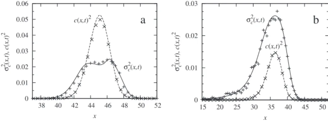
Figure1 shows the squared mean concentration and con-centration variances obtained by Laplace inversion of Eqs. 共20兲 and 共21兲 using Eq. 共22兲 for two different cut-off values 共␪c= 10, 103兲,␤= 3/2 at t=103␶vin d = 1. Notably, the uncer-tainty of concentration increases as mean transport becomes more anomalous, i.e., for increasing cut-off value ␪c. The dots denote the Monte Carlo results obtained by numerical solution of Eq.共23兲 for 103 _{particles in 2⫻10}4 _disorder

re-alizations characterized by the truncated power-law distribu-tion关Eq. 共22兲兴. The simulated behavior agrees well with the model predictions. In both cases the absolute variance in-creases as the concentration values increase. Large concen-tration values are spatially more localized than small values and thus subject to larger uncertainty. For anomalous mean transport, which is characterized by a spatial backward tail 关Fig.1共b兲兴, this behavior is amplified as the spatial distribu-tion of large concentradistribu-tion values is broader than for normal mean transport.

In conclusion, we have presented a method that allows for the determination of the full concentration statistics for trans-port in random media whose mean behavior can be modeled as a CTRW. We have studied the concentration variance for normal and anomalous mean transport behavior and have found that the concentration distribution is in general not self-averaging in the presence of an external field. Experi-mentally determined concentration values are usually ob-tained as spatial or temporal averages. Our results imply that the point values of concentration can significantly deviate

from the measured mean. Specifically, we find that the rela-tive concentration variance for anomalous mean transport be-havior is larger than the one for normal mean transport. This implies that for non-Fickian mean transport as frequently

observed in real systems, the uncertainty of the observed concentration values can be significant, which is of impor-tance for extreme value studies and risk analysis in disor-dered systems.

关1兴 H. Scher and M. Lax, Phys. Rev. B 7, 4491 共1973兲. 关2兴 R. Metzler and J. Klafter, Phys. Rep. 339, 1 共2000兲. 关3兴 J. Klafter and R. Silbey, Phys. Rev. Lett. 44, 55 共1980兲. 关4兴 J. P. Bouchaud and A. Georges, Phys. Rep. 195, 127 共1990兲. 关5兴 B. Berkowitz, A. Cortis, M. Dentz, and H. Scher, Rev.

Geo-phys. 44, RG2003共2006兲.

关6兴 M. F. Shlesinger, B. J. West, and J. Klafter, Phys. Rev. Lett.

58, 1100共1987兲.

关7兴 T. Geisel and S. Thomae, Phys. Rev. Lett. 52, 1936 共1984兲. 关8兴 P. Barthelemy, J. Bertolotti, and D. S. Wiersma, Nature

共Lon-don兲 453, 495 共2008兲.

关9兴 B. Berkowitz and H. Scher, Phys. Rev. Lett. 79, 4038 共1997兲. 关10兴 T. Le Borgne, M. Dentz, and J. Carrera, Phys. Rev. Lett. 101,

090601共2008兲.

关11兴 E. Eisenberg, S. Havlin, and G. H. Weiss, Phys. Rev. Lett. 72,

2827共1994兲.

关12兴 H. C. Fogedby, Phys. Rev. E 50, 1657 共1994兲. 关13兴 A. Baule and R. Friedrich, EPL 77, 10002 共2007兲.

关14兴 H. Risken, The Fokker-Planck Equation 共Springer, Heidelberg, NY, 1996兲.

关15兴 M. Kawasaki, T. Odagaki, and K. W. Kehr, Phys. Rev. B 61, 5839共2000兲.

关16兴 M. Dentz and A. Castro, Geophys. Res. Lett. 36, L03403 共2009兲.

关17兴 G. Margolin and B. Berkowitz, Phys. Rev. E 65, 031101 共2002兲.

关18兴 M. Dentz, A. Cortis, H. Scher, and B. Berkowitz, Adv. Water Resour. 27, 155共2004兲.

关19兴 W. Feller, An Introduction to Probability Theory and Its

Ap-plications共Wiley, New York, 1957兲, Vol. 2.

0 0.01 0.02 0.03 0.04 0.05 0.06 38 40 42 44 46 48 50 52 σ 2(x,tc ), c( x,t ) 2 x

a

σ2 c(x,t) c(x,t)2 0 0.01 0.02 0.03 15 20 25 30 35 40 45 50 σ 2 (x,tc ), c( x,t ) 2 x

b

σ2 c(x,t) c(x,t)2

FIG. 1. Concentration variances共solid lines兲 and squared mean concentrations 共dashed lines兲 in d=1 dimension obtained by inverse Laplace transform of Eqs.共20兲 and 共21兲 for the disorder distribution 关Eq. 共22兲兴 with␤=3/2 and the cut-off parameters 共a兲 ␪c= 10 and共b兲

␪c= 103. The Péclet number is Pe= 10 and the observation time t = 103␶v. The corresponding Monte Carlo results for the squared mean

concentrations共⫻兲 and concentration variances 共+兲 are obtained by numerical solution of the Langevin Eq. 共23兲 for the movements of 103

particles in each of 2⫻104_{disorder realizations. The relative variance of concentration increases as the mean transport behavior becomes}

more anomalous.

DENTZ, BOLSTER, AND LE BORGNE PHYSICAL REVIEW E 80, 010101共R兲 共2009兲