HAL Id: hal-02500116
https://hal.archives-ouvertes.fr/hal-02500116
Submitted on 26 Mar 2021
HAL is a multi-disciplinary open access
archive for the deposit and dissemination of
sci-entific research documents, whether they are
pub-lished or not. The documents may come from
teaching and research institutions in France or
abroad, or from public or private research centers.
L’archive ouverte pluridisciplinaire HAL, est
destinée au dépôt et à la diffusion de documents
scientifiques de niveau recherche, publiés ou non,
émanant des établissements d’enseignement et de
recherche français ou étrangers, des laboratoires
publics ou privés.
Influence of climate change impacts and mitigation costs
on inequality between countries
Nicolas Taconet, Aurélie Méjean, Céline Guivarch
To cite this version:
Nicolas Taconet, Aurélie Méjean, Céline Guivarch. Influence of climate change impacts and mitigation
costs on inequality between countries. Climatic Change, Springer Verlag, In press, 160, pp.15 - 34.
�10.1007/s10584-019-02637-w�. �hal-02500116�
(will be inserted by the editor)
Influence of climate change impacts and mitigation
1costs on inequality between countries
2Nicolas Taconet · Aur´elie M´ejean ·
3
C´eline Guivarch
4
5
This is the accepted version of the following article: Taconet, N., Mejean, A. & Guivarch, C. 6
Influence of climate change impacts and mitigation costs on inequality between countries. 7
Climatic Change 160, 1534 (2020). DOI: 10.1007/s10584-019-02637-w 8
Abstract Climate change affects inequalities between countries in two ways. 9
On the one hand, rising temperatures from greenhouse gas accumulation cause 10
impacts that fall more heavily on low-income countries. On the other hand, 11
the costs of mitigating climate change through reduced emissions could slow 12
down the economic catch-up of poor countries. Whether, and how much the 13
recent decline in between-country inequalities will continue in the twenty-first 14
century is uncertain, and the existing projections rarely account for climate 15
factors. In this study, we build scenarios that account for the joint effects 16
of mitigation costs and climate damages on inequality. We compute the evo-17
lution of country-by-country GDP, considering uncertainty in socioeconomic 18
assumptions, emission pathways, mitigation costs, temperature response, and 19
climate damages. We analyze the resulting 3408 scenarios using exploratory 20
analysis tools. We show that the uncertainties associated with socioeconomic 21
assumptions and damage estimates are the main drivers of future inequalities. 22
We investigate under which conditions the cascading effects of these uncer-23
tainties can counterbalance the projected convergence of countries’ incomes. 24
We also compare inequality levels across emission pathways, and analyze when 25
the effect of climate damages on inequality outweigh that of mitigation costs. 26
We stress the divide between IAM- and econometrics-based damage functions 27
in terms of their effect on inequality. If climate damages are as regressive as 28
the latter suggest, climate mitigation policies are key to limit the rise of future 29
inequalities between countries. 30
N. Taconet and C. Guivarch
ENPC, CIRED - Centre International de Recherche sur l’Environnement et le D´eveloppement. E-mail: taconet@centre-cired.fr
A. M´ejean
CNRS, CIRED - Centre International de Recherche sur l’Environnement et le D´eveloppement
Keywords Climate change · Inequality · Gini · Scenario analysis · Climate 31
mitigation · Socioeconomic scenario · Climate change impact 32
1 Introduction 33
Income inequalities between countries have declined in recent decades notably 34
as a result of rapid economic growth in China and India (Firebaugh, 2015; 35
Milanovic, 2016). Most projections see inequalities continuing along this dwin-36
dling path throughout the twenty-first century (Hellebrandt and Mauro, 2015; 37
Riahi et al., 2017; OECD, 2018; Rodrik, 2011; Hawksworth and Tiwari, 2011; 38
Spence, 2011). However, they do not consider the impact of climate change 39
on inequalities. Indeed, climate change will induce impacts that hit primarily 40
the poorest countries (Oppenheimer et al., 2014; Burke et al., 2015; Nordhaus, 41
2014; Mendelsohn et al., 2006; Stern, 2007; Tol, 2018), which may slow or even 42
reverse the expected convergence of per capita national incomes. Limiting these 43
impacts through greenhouse gas reduction policies also bears consequences for 44
inequalities, as mitigation policies could be a hurdle to development. How the 45
distributional effects of reduced climate change damages compare with those 46
of mitigation costs and how they weigh against other socioeconomic factors 47
have not been analyzed. Our paper bridges this gap. 48
We analyze how climate change affects future inequalities between coun-49
tries via joint impacts and mitigation costs. We build country-by-country GDP 50
trajectories up to 2100, exploring the uncertainty around 6 dimensions: (1) 51
socioeconomic assumptions, (2) emission pathways, (3) mitigation costs, (4) 52
regressivity of mitigation costs, (5) temperature response, (6) climate change 53
damages. The different combinations of uncertainties lead us to explore 3408 54
scenarios, for which we analyze between-country inequality as measured by 55
the Gini coefficient, as well as the first income decile. We perform a statistical 56
analysis of the outcomes to identify the main drivers of future inequality. We 57
find that the burden of climate damages on poor countries is sufficiently large 58
to lead to a reversal in the declining inequality trend in some combinations 59
of socioeconomic pathways and damage estimates. We also analyze inequality 60
levels of various emission pathways, showing that lower emissions are associ-61
ated with a lower level of inequalities under the strongest damage estimates. 62
If damage estimates are low, mitigation can still reduce inequalities in some 63
combinations of assumptions regarding socioeconomic evolution, the level of 64
mitigation cost and the distribution of these costs. 65
We discuss the drivers of future inequality in Section 2. We then present 66
the methodology used to build scenarios in Section 3. We analyze the results 67
of the projections in Section 4. We discuss limitations and conclude in Section 68
5. 69
2 Drivers of future inequality 70
We consider two types of factors affecting future economic growth: climate-71
related and socioeconomic factors. Climate change affects between-country 72
inequality in two ways: through uneven climate damages and through differ-73
entiated mitigation costs. 74
First, climate change is expected to reduce future income, through direct 75
production and capital losses and lower economic growth. It is also expected 76
to increase investment needs for adaptation. These climate damages will be 77
shared unevenly among countries, because physical impacts may differ, and be-78
cause the vulnerability to climate change and the ability to adapt vary widely 79
across countries. For instance, some countries are more dependent than others 80
on sectors that will be affected by climate change, such as the agricultural sec-81
tor. Damage evaluation is a perilous exercise: it is very difficult, if not impossi-82
ble, to predict how each country will be impacted by climate change. However, 83
an extensive literature suggests that overall damages of climate change will be 84
greater in poorer countries (Oppenheimer et al., 2014; Tol et al., 2004; Mendel-85
sohn et al., 2006; Burke et al., 2015; Nordhaus and Yang, 1996; Hallegatte and 86
Rozenberg, 2017; Dell et al., 2012), and the Intergovernmental Panel on Cli-87
mate Change lists the distribution of impacts as one of the five “Reasons for 88
Concern” about climate change. 89
Second, the cost of greenhouse gas emission reductions will affect coun-90
tries’ future income, with the costs depending on local contexts. For instance, 91
current carbon intensities differ widely across countries, as do their potentials 92
for the development of renewable energy. Mitigation policies can be more bur-93
densome for low-income countries than for rich countries, meaning that poor 94
regions may lose a greater share of GDP than rich regions for the same amount 95
of abated emissions (Krey, 2014; Edenhofer et al., 2014). Indeed, low-income 96
economies are often characterized by higher energy and carbon intensities. By 97
raising the price of energy, mitigation policies could thus hamper their ability 98
to develop. Higher costs in low-income countries can also arise due to term of 99
trade effects of climate policy (Leimbach et al., 2010). Some mitigation strate-100
gies, notably using biofuels, could also threaten food security in the poorest 101
regions (Hasegawa et al., 2018; Fujimori et al., 2019). However, the actual re-102
gressivity of mitigation costs will depend on the way the burden of the emission 103
reduction effort is shared among countries in the post-COP21 agenda (Aldy 104
et al., 2017; Liu et al., 2016) and on the feasibility of international transfers 105
(Fujimori et al., 2016). 106
Climate damages and the economic impacts of mitigation policies are 107
closely intertwined, as the greater the emission reductions through mitiga-108
tion policies, the smaller the damages. Thus, while greenhouse gas emission 109
reduction may place a greater burden on poor countries, it also reduces future 110
damages that fall disproportionately on them, so that the resulting effect of 111
mitigation is ambiguous in terms of inequality: avoided climate change may 112
reduce inequality only if mitigation costs do not fall too heavily on the poor-113
est countries. Yet, no study has brought both sides of the issue together to 114
study future inequalities. Here, we analyze inequalities between countries for 115
different emission pathways. 116
Climate-related factors are only one piece of the future inequality puzzle, 117
as other socioeconomic factors affect the gap between rich and poor coun-118
tries, such as demographics, technological progress, education, and institu-119
tions (Barro and Sala-i Martin, 2004). A key question concerns the ability of 120
Table 1 The Shared Socioeconomic Pathways (SSP)
SSP Name
1 Sustainability
2 Middle of the Road
3 Regional Rivalry
4 Inequality
5 Fossil-fueled Development
low income countries to mimic China and India’s rapid economic catch-up. 121
Whether convergence is just a question of time, occurs only regionally or is 122
country-specific is the subject of intense debates in the development literature 123
(Milanovic, 2006; Rodrik, 2011), and how fast the income of different countries 124
can converge in the twenty-first century remains deeply uncertain. 125
3 Methodology 126
3.1 Building the scenarios 127
We build scenarios to explore future inequalities between countries, account-128
ing for socioeconomic and climate-related factors. We model 6 dimensions of 129
uncertainties: (1) socioeconomic assumptions, (2) emission pathways, (3) mit-130
igation cost estimates, (4) regressivity of mitigation costs, (5) temperature 131
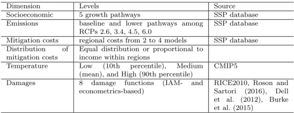
response, (6) climate change damages. A summary of the uncertainties and 132
sources considered is provided in table 2. 133
134
3.1.1 Socioeconomic assumptions 135
We use shared socioeconomic pathways (SSP) scenarios to explore possible 136
evolutions of socioeconomic factors in the twenty-first century (Riahi et al., 137
2017). SSPs consist of five pathways (SSPs 1 to 5) that reflect combined and 138
consistent hypotheses on demographics, technological progress, and socioeco-139
nomic evolutions (see table 1). SSPs project economic growth for all countries 140
based on future population, technological progress, physical and human capi-141
tal, as well as energy and fossil resources (Dellink et al., 2017). While SSPs 1 142
and 5 depict sustained growth and convergence of income levels by the end of 143
the century, in SSPs 3 and 4 poor prospects for developing countries and lack 144
of cooperation lead to much slower reduction of inequality. SSP 2 lies in be-145
tween, with moderate growth and convergence. For each country, initial GDP 146
per capita levels in 2015 are set using the latest World Development Indicators 147
(WDI 2017, May), and economic growth is set based on SSP trajectories.1
148
3.1.2 Emission pathways 149
The SSP growth projections for all countries assume there are no climate policy 150
and no climate change impacts. We build on these projections to compute 151
projections for different mitigation pathways with radiative forcing targets 152
corresponding to representative concentration pathways (RCPs). The radiative 153
forcing levels reached in the baseline case in 2100 differ across SSPs, with the 154
highest — SSP 5 — being the only one above RCP 8.5, while the lowest — 155
SSP 1 — is below RCP 6.0 (Riahi et al., 2017). Thus, we leave aside RCP 156
8.5, and only keep RCPs 2.6, 4.5, and 6.0, to which we add the intermediary 157
radiative forcing target of 3.4 W/m2 from the SSP database. Of these, only
158
RCP 2.6 is likely to meet the target of limiting global mean temperature 159
increase below 2◦C compared with pre-industrial levels (Stocker et al., 2013).
160
For all mitigation scenarios, we account for mitigation costs to meet the target 161
and for the economic impacts from a changing climate. 162
3.1.3 Mitigation costs 163
We compute mitigation costs based on regional projections from the SSP 164
database, which provides the results from six different integrated assessment 165
models (IAMs) for scenarios spanning the SSP-RCP matrix. We use mitiga-166
tion costs calculated by the IAMs that include an endogenous growth module 167
(AIM/GCE, MESSAGE-GLOBIUM, REMIND-M, and WITCH). Other IAMs 168
in the SSP database (IMAGE and GCAM) assume exogenous GDP growth 169
pathways that are not affected by mitigation policies and thus do not change 170
according to the RCP. We exclude the results from these models, as they do 171
not represent the effect of mitigation on growth. Of the four models, some have 172
not run all SSPs, so we have between 2 and 4 estimates for each combination 173
of SSP/RCP. A clear advantage of using the mitigation costs from the SSP 174
database is that they are consistent with the storylines of the SSPs. Thus, the 175
same target is more difficult to reach in a scenario where baseline emissions 176
are large or technical progress is slow. However, the cost projections rely on a 177
least-cost approach, which brings two caveats. First, the actual cost of reaching 178
the target may in fact be higher due to real-world market imperfections, for 179
instance if there is inertia or imperfect foresight (Waisman et al., 2012). Sec-180
ond, emission reductions are supposed to take place in the region where they 181
are the cheapest, regardless of equity considerations. Given the limited coop-182
eration and policy harmonization across countries on climate change issues at 183
present, the distribution of costs may differ from those assumed in the SSP 184
database. To account for different effort-sharing schemes, we use two variants 185
of mitigation cost distribution: first, we distribute the regional costs from the 186
IAMs within each region proportionally to each country’s income. Second, we 187
look at the more regressive case of equally-shared costs within a region. As we 188
explain in section 5.1, more progressive distributions could be envisaged that 189
would reflect different burden sharing approaches under international negoti-190
ations. Such distribution would strengthen the impact of climate damages on 191
inequality relative to mitigation cost. 192
3.1.4 Temperature response 193
There is great variability in the evolution of temperature at the country level 194
for a given RCP as given by climate models (Stocker et al., 2013). Therefore, 195
we consider values for temperature changes corresponding to the mean, and the 196
10th and 90th percentile of outcomes. Temperature changes in 2100 are taken 197
from the Climate Intercomparison Model Project CMIP52. CMIP5 provides
198
national mean annual temperature changes in 2100 for RCPs 2.6, 4.5, 6.0 and 199
8.5. When the radiative forcing in 2100 of a scenario falls between two values 200
provided by CIMP5, we perform a linear interpolation to calculate temperature 201
change in 2100. Using the 2100 value, we assume that temperatures increase 202
linearly over time. 203
3.1.5 Climate change damages 204
Given that future climate change damages are very uncertain, we use 8 esti-205
mates from different sources for damages associated with different temperature 206
changes, from Integrated Assessment Models, and from the econometrics lit-207
erature. 208
Integrated assessment models are primarily used to analyze the interac-209
tion between climate and the economy (Nordhaus, 2008). In particular, they 210
are used to derive optimal emissions pathways balancing the cost of mitiga-211
tion with the benefits of avoided damages. However, they typically provide 212
global damage estimates – and the damage estimates they rely on are global, 213
too. RICE and FUND are notable exceptions: we therefore use estimates from 214
RICE2010 (Nordhaus, 2014).3 We also draw upon estimates relying on the
215
GTAP model (Global Trade Analysis Project). Roson and Sartori (2016) (RS 216
hereafter) assess the economic changes associated with higher temperature in 217
different sectors (agriculture, health, tourism...) for 140 regions. We use their 218
aggregate estimates of the percentage change of GDP in a 3◦C scenario
com-219
pared with the associated baseline, for the different regions. This percentage 220
GDP change may be positive or negative depending on the region. We assume 221
that this effect on GDP grows proportionally with global temperature. 222
Finally, we use estimates from the econometrics literature, which shows ev-223
idence that temperature changes have impacted economic growth in the past, 224
and more heavily so in poorer countries. This difference is attributed either to 225
national development levels (Dell et al., 2012), or to mean temperature (Burke 226
et al., 2015). Burke et al. (2015) (BHM hereafter) derive a damage function 227
from historical GDP and temperature data. The authors econometrically es-228
timate the effect of higher than average annual temperature, controlling for 229
2
https://climexp.knmi.nl/plot_atlas_form.py
other variables. They find a non-linear bell-shaped relationship between tem-230
perature and economic growth, showing a maximum for an annual average 231
temperature of around 13◦C.
232
Additionally, we consider econometric estimates from Dell et al. (2012) 233
(DJO hereafter), who find a strong and significant effect of temperature on 234
growth in poor countries, while the effect for rich countries is small. We ac-235
count for the future divide between rich and poor countries in two ways: (1) 236
a static version, where poor countries are defined as those currently below 237
median income, a definition that is set over the whole horizon, (2) a dynamic 238
version, with current median income defining the threshold between poor and 239
rich countries, thus allowing countries to switch status over time. This second 240
version accounts for some form of adaptation where income growth compen-241
sates (here almost fully) the negative impact of climate change. 242
For both damage functions, we use the regressions with 0 and 5-year lags. 243
A distributed lag model with 5-lags adds up the effect of temperature in the 244
current and 5 previous years. This allows capturing the cumulative effect of 245
temperature on income rather than solely a short-run effect. We discuss the 246
limitations of relying on econometric estimates to project future damages in 247
section 5.1. 248
3.1.6 Computing economic growth 249
Using mitigation costs and climate damages for each country, GDP per capita 250
Y at time t in a given RCP scenario is calculated as follows, for RICE and 251
RS: 252
Yt,RCP = Xt,RCPΩ(GM Tt)Yt,baseline (1)
where Xt,RCP is the mitigation cost factor, Ω(GM Tt) is the damage factor
253
in the region for a global mean temperature change of GM Tt, and Yt,baseline
254
is the GDP per capita in the corresponding baseline scenario. 255
For econometrics-based damage functions (BHM and DJO), the equation 256
writes: 257
Yt,RCP = Xt,RCP(1 + gt,baseline+ ∆g(Tt))Yt−1,RCP (2)
where gt,baseline is the growth projected in a baseline without climate
im-258
pacts and ∆g(Tt) is the loss of economic growth under national temperature
259
Ttdue to climate change.
260
In total, we are able to compute the projections for 161 countries, currently 261
representing 96% of world population. We exclude countries for which we lack 262
either initial GDP or future temperature projections. 263
The combination of different socioeconomic assumptions (5 SSPs), emis-264
sions pathways (baseline and between 2 and 4 RCPs, depending on the SSP), 265
mitigation costs estimates (2 to 4 estimates depending on the SSP and RCP, 266
with 2 variants of the distribution of costs within region for each estimate), 267
temperature response to a given RCP (3 cases), and damage estimates (8 268
Table 2 Uncertain factors considered in the study
Dimension Levels Source
Socioeconomic 5 growth pathways SSP database
Emissions baseline and lower pathways among
RCPs 2.6, 3.4, 4.5, 6.0
SSP database Mitigation costs regional costs from 2 to 4 models SSP database Distribution of
mitigation costs
Equal distribution or proportional to income within regions
Temperature Low (10th percentile), Medium
(mean), and High (90th percentile)
CMIP5
Damages 8 damage functions (IAM- and
econometrics-based)
RICE2010, Roson and Sartori (2016), Dell et al. (2012), Burke et al. (2015)
models) results in 3408 scenarios. Scenarios are consistent in the sense that 269
for each combination, the mitigation costs are those estimated for the corre-270
sponding SSP/RCP, while climate damages are calculated according to the 271
temperature change induced by the emission pathway against the tempera-272
ture response. However, we ignore the fact that damages that damages for 273
a given temperature change may also depend on the socioeconomic pathway. 274
This limitation is discussed in section 5.1. Besides, some combinations of fac-275
tors may be more plausible than others, but we nevertheless consider all of 276
them without making a priori judgements about their likelihood. 277
3.2 Measuring income inequality 278
The literature distinguishes three types of income inequality (Milanovic, 2011): 279
(1) unweighted international inequality compares countries’ income regardless 280
of their size, (2) population-weighted international inequality weighs countries’ 281
income according to their population (3) total inequality accounts for house-282
holds’ or individuals’ revenue distributions within and across countries. We 283
focus on the second type of inequality, which gives equal weight to all indi-284
viduals across countries. This choice of international inequality is motivated 285
as follows. First, between-nation inequality represents, as of today, the great-286
est source of inequality between individuals (Firebaugh, 2015; Bourguignon 287
and Morrisson, 2002). Besides, future income distribution within a country is 288
subject to policy choices that would be difficult to model. 289
Many indicators can be used to measure this type of inequality (Charles-290
Coll, 2011). The most routinely used index is the Gini index, which computes 291
the dispersion of income, ranging from 0 (perfect equality) to 1 (one individual 292
or entity owns all the income). The Gini index is the ratio of the mean absolute 293
difference between two individuals or entities to twice the mean level of income. 294
If countries indexed by i are ranked based on their per capita income Ii, with
295
pi their population, we can define the cumulated proportion of income and
296
population as follows: 297
pc,i= Pi k=1pk PN k=1pk (3) Ic,i= Pi k=1Ik PN k=1Ik (4) The Gini index then writes:
298
Gini = 1 − N X
k=i
(pc,i− pc,i−1)(Ic,i− Ic,i−1) (5)
with Ic,0 = 0 and pc,0 = 04. Appealing for its simplicity, the Gini index
299
is also criticized, notably because it may be regarded as overly sensitive to 300
changes in the middle of the distribution, and because it measures relative 301
inequality (Cowell, 2000). Indeed, a world with more inequality may still be 302
better for the poorest in absolute terms. Thus, we also examine the absolute 303
situation of the bottom 10%, as measured by the first income decile (see section 304
4.4). 305
4 Results 306
We compute the Gini index in all scenarios, and analyze the drivers of its 307
evolution over the twenty-first century. 308
4.1 A trend reversal in inequalities 309
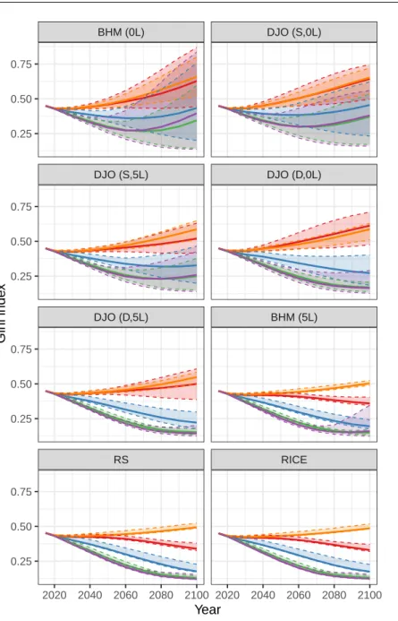
Both socioeconomic and climate-related uncertainties strongly influence the 310
evolution of future inequalities (figure 1). In many scenarios, inequalities con-311
tinue to decline for a few years or decades, but as climate change impacts 312
gradually occur, they may outweigh the forecasted economic catch-up by low-313
income countries, and inequalities may rise again as a result. 314
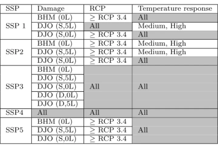
We perform a PRIM analysis to identify the combinations of uncertainties 315
that lead to this trend reversal, using the method described in Guivarch et al. 316
(2016)5. The results of this analysis show that there are cases of trend reversal
317
in all socioeconomic pathways, even in the most optimistic ones (see table 3). 318
Inequalities rise again systematically in SSP 4, a socioeconomic world depict-319
ing a great divide between rich and poor countries. With the low prospect 320
for catch-up assumed in SSP 3, a trend reversal in inequality can also occur, 321
but only for high damage estimates (namely BHM (0 lag), and all DJO es-322
timates). For other socioeconomic pathways, regressive damage specifications 323
4 The pairs (p
c,i,Ic,i) represent the Lorenz curve: a proportion pc,iof the population earns a proportion Ic,i of global income. Graphically, the Gini coefficient is worth half the area between the Lorenz curve and the first bisector.
RS RICE DJO (D,5L) BHM (5L) DJO (S,5L) DJO (D,0L) BHM (0L) DJO (S,0L) 2020 2040 2060 2080 2100 2020 2040 2060 2080 2100 0.25 0.50 0.75 0.25 0.50 0.75 0.25 0.50 0.75 0.25 0.50 0.75 Year Gini inde x Socioeconomic pathway (SSP) 1. Sustainability 2. Middle of the Road 3. Regional Rivalry 4. Inequality
5. Fossil−fueled Development
Fig. 1 Evolution of the Gini index over time. A panel corresponds to a damage function. For each socioeconomic pathway, the dotted lines represent the minimum and maximum values of the Gini index, while the plain line is the mean. ’DJO’: Dell et al. (2012), ’BHM’: Burke et al. (2015), ’RS’: Roson and Sartori (2016). For DJO, ’S’ and ’D’ stand respectively for static and dynamic poor/rich distinction. For DJO and BHM, ’0L’ and ’5L’ refer to 0-year lag or 5-year lag regression.
Table 3 Each line is a combination where a trend reversal in the Gini occurs, of factors leading to a trend reversal in inequality, as revealed by PRIM analysis. The trend reversal can occur in all SSPs, but in some SSPs only for high damages, a high RCP or a high temperature response.
SSP Damage RCP Temperature response
BHM (0L) ≥ RCP 3.4 All
DJO (S,5L) All Medium, High
SSP 1
DJO (S,0L) ≥ RCP 3.4 All
BHM (0L) ≥ RCP 3.4 Medium, High
DJO (S,5L) ≥ RCP 3.4 Medium, High
SSP2 DJO (S,0L) ≥ RCP 3.4 All BHM (0L) DJO (S,5L) DJO (S,0L) DJO (D,0L) SSP3 DJO (D,5L) All All
SSP4 All All All
BHM (0L) ≥ RCP 3.4
DJO (S,5L) ≥ RCP 3.4
SSP5
DJO (S,0L) ≥ RCP 3.4
All
(i.e. econometrics-based) slow down the convergence, and make inequalities 324
rise again under strong temperature change (either because of high emission 325
or high temperature response). 326
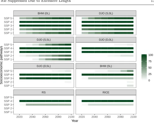
In the cases where inequalities rise again, the timing of the trend reversal 327
also varies depending on the uncertainties, in particular the combination of 328
socioeconomic assumptions and damage function (see figure 2). The reversal 329
occurs systematically as early as in the 2020s in SSP 4. In SSP 3, the occur-330
ring decade is determined by the damage estimates, but varies between lowest 331
and highest damage estimates. For the more ’optimistic’ socioeconomic path-332
ways (SSPs 1, 2 and 5), there is great variability in the date at which the 333
trend reversal occurs for high damage estimates. In such cases, lower emission 334
scenarios or low temperature response scenarios delay the reversal. 335
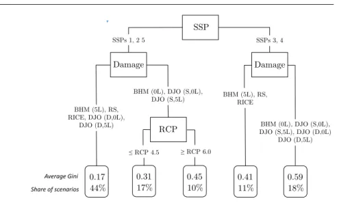
4.2 Analyzing the Gini index using regression trees 336
We analyze how the different uncertainties affect the Gini index, and we com-337
pute a regression tree to identify the main drivers of its value in 2100. We use 338
recursive partitioning to select the factors in order to reduce the heterogeneity 339
of the output value.6The regression tree identifies socioeconomic assumptions
340
(SSPs) and the damage function as the first two nodes of the decision tree, 341
suggesting that these dimensions are the most influential on inequalities in 342
2100 (figure 3). The first node splits the scenarios into two groups, the first 343
one composed of scenarios with ’optimistic’ socioeconomic assumptions (SSPs 344
1,2 and 5) in terms of convergence between poor and rich countries, and the 345
6 We used rpart function of R (complexity parameter of rpart function is set at 0.02, meaning that a split is retained if it increases the fit by a factor 0.02)
RS RICE DJO (D,5L) BHM (5L) DJO (S,5L) DJO (D,0L) BHM (0L) DJO (S,0L) 2020 2040 2060 2080 2100 2020 2040 2060 2080 2100 SSP 1 SSP 2 SSP 3 SSP 4 SSP 5 SSP 1 SSP 2 SSP 3 SSP 4 SSP 5 SSP 1 SSP 2 SSP 3 SSP 4 SSP 5 SSP 1 SSP 2 SSP 3 SSP 4 SSP 5 Year Socioeconomic pathw a ys 0 25 50 75 100
Fig. 2 Cumulated percentage of scenarios where a trend reversal has occurred, for a given combination of damage function and socioeconomic assumptions.
second one composed of scenarios with pessimistic such assumptions (SSPs 346
3 and 4). Within each branch, the tree further splits scenarios according to 347
the magnitude of climate change damages. Interestingly, the grouping of the 348
damage functions differs across the two branches of the tree. Indeed, when the 349
vulnerability of countries depends on their income (in the ’dynamic’ versions of 350
DJO), climate damages strongly depend on the socioeconomic pathway: con-351
vergence assumptions limit the effect of climate change on inequalities, because 352
poor countries can shield themselves from climate damages through develop-353
ment. The contrary holds if poor countries are assumed to slowly catch-up 354
with rich countries. Finally, if optimistic SSPs are combined with high dam-355
ages, the next node splits the remaining scenarios according to the level of 356
emissions. All the other dimensions of uncertainties, that is mitigation costs, 357
their distribution within regions, as well as temperature response uncertainty, 358
contribute to a lesser extent to the Gini index in 2100. 359
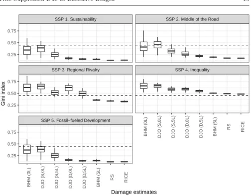
For the highest damage estimates (i.e. mostly econometric estimates), the 360
cascading effect of emission pathway and temperature response uncertainty 361
translate into great variability in the benefits of avoided damages for the poor-362
est, and thus a greater variability of the Gini index in 2100 (figure 4). With 363
the most regressive specifications, damages are such that they may completely 364
cancel out expected convergence in some scenarios, and lead to a higher Gini 365
SSP Damage RCP Damage 0.17 44% 0.31 17% 0.45 10% 0.41 11% 0.59 18% SSPs 1, 2 5 SSPs 3, 4 BHM (0L), DJO (S,0L), DJO (S,5L) BHM (0L), DJO (S,0L), DJO (S,5L), DJO (D,0L) DJO (D,5L) BHM (5L), RS, RICE BHM (5L), RS, RICE, DJO (D,0L), DJO (D,5L) ≥ RCP 6.0 ≤ RCP 4.5 Average Gini Share of scenarios
Fig. 3 Regression tree on the value of Gini in 2100. The algorithm splits scenarios to best predict the value of the output, thus generating groups with minimal heterogeneity. In each leaf of the tree, the upper number is the mean of Gini for the scenarios in the box, while the lower number is the percentage of scenarios it represents.
index in 2100 than today. In particular in SSP3, most scenarios with econo-366
metric damage estimates show Gini levels higher than today, while it is not 367
the case under low damage functions. Gini index can be higher than today 368
in other socioeconomic pathways, but only when combining the most regres-369
sive damage functions (BHM (0L) and DJO (S,0L)) with the highest emission 370
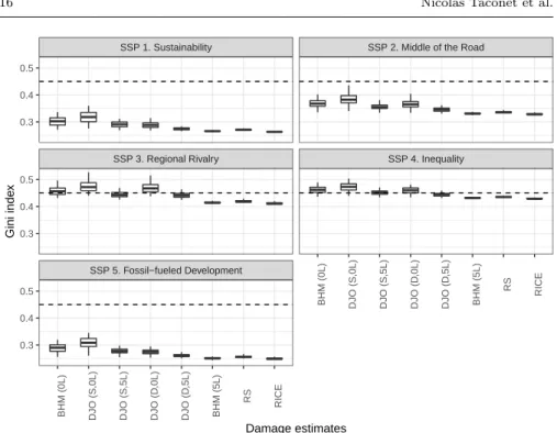
pathways. However, in the short run (the Gini index in 2050 is shown in figure 371
5), socioeconomic assumptions appear as the main drivers of inequalities, with 372
limited variability across other dimensions. 373
4.3 Does mitigation reduce inequalities? 374
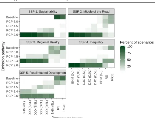
We compare inequality levels in 2100 across emissions pathways to analyze 375
how the regressive impacts of climate damages compare to those of mitigation 376
costs. We analyze which emission pathway, all else being equal, has the lowest 377
inequality level (figure 6). Unsurprisingly, lower emission pathways are pre-378
ferred when assuming regressive damages. We look specifically for the cases in 379
which RCP 2.6 is the preferred emission pathway, because it is the only RCP 380
likely to achieve the 2◦C target.7 Whether RCP 2.6 performs best in terms of
381
inequality depends primarily on the damage function. With the most regres-382
sive damage estimates (BHM, 0L), inequalities are always lowest under RCP 383
7 Note that models have not produced this emission pathway under the most pessimistic socioeconomic pathway (SSP 3), where low growth is combined with high challenge to mit-igation
SSP 5. Fossil−fueled Development
SSP 3. Regional Rivalry SSP 4. Inequality SSP 1. Sustainability SSP 2. Middle of the Road
BHM (0L) DJO (S ,0L) DJO (S ,5L) DJO (D ,0L) DJO (D ,5L) BHM (5L) RS RICE BHM (0L) DJO (S ,0L) DJO (S ,5L) DJO (D ,0L) DJO (D ,5L) BHM (5L) RS RICE 0.25 0.50 0.75 0.25 0.50 0.75 0.25 0.50 0.75 Damage estimates Gini inde x
Fig. 4 Boxplot of the Gini index in 2100, for combinations of socioeconomic assumptions (panel) and damage functions (x-axis)
2.6 unless the high baseline emissions of SSP 5 is combined with the highest 384
mitigation costs estimates (WITCH). Under the other econometric damage 385
estimates, RCP 2.6 is the less unequal emission pathway either for optimistic 386
SSPs with low challenges to mitigation (1, 2, 4), or when mitigation costs are 387
low (all except WITCH). RCP 2.6 is less often the scenario with the lowest 388
inequality levels IAM-based damage functions, i.e. RICE and RS. Netherless, 389
even under low damage estimates, RCP 2.6 may still be the emission pathway 390
with the lowest inequality level in some specific combinations, in particular for 391
optimistic SSPs, provided that mitigation costs are not shared evenly within 392
regions. 393
Likewise, looking at SSP 3, the damage estimate also primarily drives the 394
comparison across emission pathways, and the same pattern can be observed. 395
For high damages, avoided damages outweigh the cost to keep emissions com-396
patible with RCP 3.4, while the contrary holds in the case of lower damages. 397
Given that SSP 3 depicts a low-growth, low-technical progress world, mitiga-398
tion is particularly costly, so that the lowest inequality levels do not always 399
coincide with the lowest emission pathway. 400
SSP 5. Fossil−fueled Development
SSP 3. Regional Rivalry SSP 4. Inequality SSP 1. Sustainability SSP 2. Middle of the Road
BHM (0L) DJO (S ,0L) DJO (S ,5L) DJO (D ,0L) DJO (D ,5L) BHM (5L) RS RICE BHM (0L) DJO (S ,0L) DJO (S ,5L) DJO (D ,0L) DJO (D ,5L) BHM (5L) RS RICE 0.3 0.4 0.5 0.3 0.4 0.5 0.3 0.4 0.5 Damage estimates Gini inde x
Fig. 5 Boxplot of the Gini index in 2050, for combinations of socioeconomic assumptions (panel) and damage functions (x-axis)
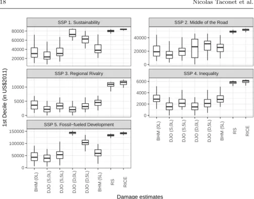
4.4 Does mitigation improve the situation of the poorest? 401
The Gini index only provides a relative measure of inequality, and thus does not 402
give information about the absolute situation of the poorest. Here, we compute 403
the first income decile in 2100, which reflects the situation of the poorest 10% 404
(figure 7). Socioeconomic assumptions appear as the first driver of the situation 405
of the poorest 10%, as it is the case with the Gini index, with differences larger 406
than one order of magnitude across SSPs. There are also strong discrepancies 407
between damage functions, and the most regressive results in terms of Gini 408
are not necessarily the ones for which the situation of the poorest is the worst. 409
However, the first income decile is almost systematically larger under RICE 410
and RS damages than for econometrics-based damage functions. 411
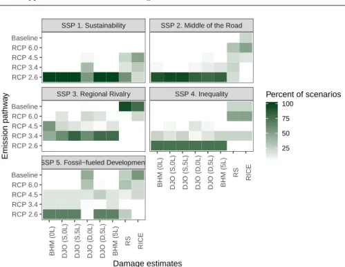
We also compare the first income decile across emissions pathways (see 412
figure 8). The distribution of the preferred emission pathway based on the value 413
of the first income decile is generally close to that based on the Gini index. 414
As it was the case for inequality, the situation of the poorest 10% tends to be 415
better in lower emission pathways for econometrics-based damage functions. 416
However, for the dynamic specification of DJO (0-lag) in high-growth SSP 5, 417
rapid convergence allows the poorest 10% to become less vulnerable to climate 418
change, so that mitigation does not improve their situation. Even under RICE 419
SSP 5. Fossil−fueled Development
SSP 3. Regional Rivalry SSP 4. Inequality SSP 1. Sustainability SSP 2. Middle of the Road
BHM (0L) DJO (S ,0L) DJO (S ,5L) DJO (D ,0L) DJO (D ,5L) BHM (5L) RS RICE BHM (0L) DJO (S ,0L) DJO (S ,5L) DJO (D ,0L) DJO (D ,5L) BHM (5L) RS RICE RCP 2.6 RCP 3.4 RCP 4.5 RCP 6.0 Baseline RCP 2.6 RCP 3.4 RCP 4.5 RCP 6.0 Baseline RCP 2.6 RCP 3.4 RCP 4.5 RCP 6.0 Baseline Damage estimates Emission pathw a y 25 50 75 100 Percent of scenarios
Fig. 6 Which emission pathway has the lowest inequality level? We compare inequality levels across emission pathways, all else being equal. The graph shows the percentage of scenarios in which each emission pathway has the lowest inequality level. We group scenarios based on SSP (panel) and damage estimates (x-axis). For instance, in SSP 1 and under BHM (0L) damages, RCP 2.6 always has the lowest Gini.
damages, the first income decile can be higher for higher emission pathways. 420
It is the case for SSPs where a significant number of countries stay behind 421
(SSPs 3 and 4); and in SSPs 2 and 5, although only under low or moderate 422
temperature response. Finally, with RS damages function, the poorest 10% 423
are better off without mitigation if we assume low growth (SSP 3) or high 424
mitigation costs (WITCH). 425
5 Discussion 426
5.1 Limitations of the study 427
Our results are conditional on the relative magnitude of the mitigation and 428
damage cost estimates we use, as well as on their distribution across countries. 429
We highlight that many outcomes regarding future inequality will depend on 430
the level of damages. Although we have tried to include as many estimates 431
as possible in the analysis, IAM-based and econometrics damages all have 432
limitations (Diaz and Moore, 2017). Econometrics-based damage functions 433
SSP 5. Fossil−fueled Development
SSP 3. Regional Rivalry SSP 4. Inequality SSP 1. Sustainability SSP 2. Middle of the Road
BHM (0L) DJO (S ,0L) DJO (S ,5L) DJO (D ,0L) DJO (D ,5L) BHM (5L) RS RICE BHM (0L) DJO (S ,0L) DJO (S ,5L) DJO (D ,0L) DJO (D ,5L) BHM (5L) RS RICE 0 20000 40000 0 2000 4000 6000 20000 40000 60000 80000 0 5000 10000 0 50000 100000 150000 Damage estimates
1st Decile (in US$2011)
Fig. 7 Boxplot of the 1st income decile in 2100, for combinations of socioeconomic assump-tions (panel) and damage funcassump-tions (x-axis). Note that the scale of the y-axis differs across panels.
represent a large share of the estimates used here. Although they allow for an 434
empirically-grounded country-by-country treatment of damages, the validity 435
of extrapolating into the future the short-term effects of weather on economic 436
growth to assess the economic impact of climate change is subject to debate 437
(Schlenker and Auffhammer, 2018). On the one hand, long-term adaptation 438
may occur and reduce negative impacts. On the other hand, impacts could 439
be exacerbated by non-linear effects outside of historical experience and by 440
other potential sources of economic loss associated with climate change but 441
not linked to temperature change, such as sea-level rise. Which of these two 442
effects will prevail remains uncertain. 443
Another, related, limitation is the difficulty to account for the vulnerability 444
of countries, as well as their ability to adapt to climate change in different 445
socioeconomic pathways. Depending on the socioeconomic pathway, it may be 446
more or less challenging – and thus costly – to adapt to a given temperature 447
change. We account for some form of adaptation in the dynamic version of 448
DJO damages, where damages depend on the level of income of the country. 449
However, we do not proceed likewise for the other damage cases. Exploring 450
in a more sophisticated manner the ability of future societies to cope with 451
temperature changes would greatly improve the study, and strengthen the 452
SSP 5. Fossil−fueled Development
SSP 3. Regional Rivalry SSP 4. Inequality SSP 1. Sustainability SSP 2. Middle of the Road
BHM (0L) DJO (S ,0L) DJO (S ,5L) DJO (D ,0L) DJO (D ,5L) BHM (5L) RS RICE BHM (0L) DJO (S ,0L) DJO (S ,5L) DJO (D ,0L) DJO (D ,5L) BHM (5L) RS RICE RCP 2.6 RCP 3.4 RCP 4.5 RCP 6.0 Baseline RCP 2.6 RCP 3.4 RCP 4.5 RCP 6.0 Baseline RCP 2.6 RCP 3.4 RCP 4.5 RCP 6.0 Baseline Damage estimates Emission pathw a y 25 50 75 100 Percent of scenarios
Fig. 8 What is the most favorable emission pathway in terms of the situation of the poorest 10%? We compare first income decile levels across emission pathways, all else being equal. The graph shows the percentage of scenarios in which each emission pathway has the greater first income decile. We group scenarios based on SSP (panel) and damage estimates (x-axis). For instance, in SSP 1 and with BHM (0L) damages, RCP 2.6 is always the emission pathway in which the situation of the poorest 10% is the best.
role of the socioeconomic pathway, as it does in the dynamic setting of DJO 453
damages, but it would also increase its complexity. 454
The magnitude of the actual macroeconomic mitigation costs may also 455
exceed the evaluations given by IAMs that quantified the SSPs, in particu-456
lar considering real-world frictions and second-best mechanisms which were 457
not accounted for by those models (Guivarch et al., 2011). In addition, the 458
distribution of mitigation costs among countries will ultimately result from 459
the relative ambition for emissions reduction as defined by their nationally 460
determined contribution to the Paris Agreement, the stringency of policies 461
implemented to reach those, and international climate finance and technology 462
transfer mechanisms (Aldy et al., 2016). The distribution of costs may there-463
fore be more or less regressive than the distribution implied by the mitigation 464
policies represented by the IAMs in the SSP database. Many effort-sharing 465
approaches, for instance accounting for historical responsibility, lead to more 466
stringent targets for developed countries, suggesting that international nego-467
tiations may lead to distributions that are less regressive than cost-optimal 468
approaches (van den Berg et al., 2019). Considering such cases would reduce 469
the burden of mitigation on poor countries, and thus reinforce the result that 470
mitigation can reduce inequalities. 471
Considering inequalities among individuals (Dennig et al., 2015; Alvaredo 472
et al., 2018) and not only between countries, and accounting for dimensions of 473
inequality beyond income, such as health inequalities, would complement our 474
analysis of the inequality implications of climate change damages and mitiga-475
tion. Such extensions would bring further complexity, but have the potential 476
to amplify the results because poor households are particularly vulnerable to 477
climate change impacts (Hallegatte and Rozenberg, 2017). Health inequalities 478
would probably worsen under severe climate change, since health impacts due 479
to climate change disproportionally affect the poor (Patz et al., 2005; Haines 480
et al., 2006), and mitigation generally results in health co-benefits (Smith 481
et al., 2014). 482
5.2 Conclusion 483
We study how greenhouse gas reduction may affect inequality through mit-484
igation costs and avoided climate damages, with effects going in opposing 485
directions. We build scenarios to account for their influence on future inequal-486
ities, and explore uncertainties along different dimensions: socioeconomic as-487
sumptions, emission pathways, mitigation costs, the regressivity of mitigation 488
costs, temperature response, and climate change damages. We show that so-489
cioeconomic assumptions and climate change damages are the main drivers of 490
the outcomes in the long term. The emission pathway also influences future 491
inequalities, while the temperature response, the mitigation costs and their 492
distribution play a lesser role. In most scenarios, inequalities among countries 493
decline in the short to medium run, but can start rising again as climate change 494
impacts gradually outweigh the expected economic convergence between low-495
and high-income countries. We show this occurs systematically in scenarios as-496
suming low socioeconomic convergence between rich and poor countries (SSP 497
4). It can occur in all other socioeconomic pathways when considering high 498
(i.e. econometrics-based) damage, but only under the most pessimistic temper-499
ature responses or the highest emission pathways. Whether mitigation reduces 500
inequalities depends primarily on damage estimates. Under the highest dam-501
age estimates, it is very likely that inequalities may rise again, in particular 502
in socioeconomic pathways with rather low challenge to mitigation, and when 503
mitigation costs estimates are low. Mitigation can also reduce inequalities un-504
der less regressive damage functions, though under more specific assumptions 505
regarding socioeconomic evolution and mitigation costs. In such scenarios, the 506
benefits of avoided damages dominate the regressive effect of climate poli-507
cies. The same drivers play a crucial role when looking at the situation of the 508
poorest 10%, and the benefits of avoided damages on the first income decile 509
outweigh those of mitigation costs in the same scenarios. 510
Our results are subject to several caveats and should be interpreted with 511
caution. Nonetheless, they indicate that the cascading uncertainties in emis-512
sion pathways, temperature and damage estimates can lead the distributional 513
impacts of future climate change to counterbalance the projected conver-514
gence of countries’ incomes. We further stress the divide between IAM- and 515
econometrics-based damage functions, showing that they do not only differ 516
in terms of the aggregate level of damage, but also in terms of their effect 517
on inequality. If climate change is as regressive as econometrics-based damage 518
functions suggest, climate mitigation policies are key to limit the rise of future 519
inequalities between countries. 520
Acknowledgements The authors would like to thank three anonymous reviewers for their 521
very valuable feedbacks. The authors would also like to thank St´ephane Hallegatte, Eloi 522
Laurent, Louis-Ga¨etan Giraudet and participants to the 2018 EAERE-VIU-FEEM Summer 523
School on Climate Change Assessment in Venice. The authors acknowledge funding pro-524
vided by the NAVIGATE project (H2020/20192023, grant agreement number 821124) of 525
the European Commission. 526
References 527
Aldy J, Pizer W, Tavoni M, Reis LA, Akimoto K, Blanford G, Carraro C, 528
Clarke LE, Edmonds J, Iyer GC (2016) Economic tools to promote trans-529
parency and comparability in the Paris Agreement. Nature Climate Change 530
6(11):1000 531
Aldy JE, Pizer WA, Akimoto K (2017) Comparing emissions mitigation ef-532
forts across countries. Climate Policy 17(4):501–515, DOI 10.1080/14693062. 533
2015.1119098, URL https://doi.org/10.1080/14693062.2015.1119098 534
Alvaredo F, Chancel L, Piketty T, Saez E, Zucman G (2018) World Inequality 535
Report 2018. Tech. rep., URL http://wir2018.wid.world/ 536
Barro RJ, Sala-i Martin X (2004) Economic Growth: MIT Press. Cambridge, 537
Massachusettes 538
van den Berg NJ, van Soest HL, Hof AF, den Elzen MGJ, van Vuuren DP, Chen 539
W, Drouet L, Emmerling J, Fujimori S, Hhne N, Kberle AC, McCollum 540
D, Schaeffer R, Shekhar S, Vishwanathan SS, Vrontisi Z, Blok K (2019) 541
Implications of various effort-sharing approaches for national carbon budgets 542
and emission pathways. Climatic Change DOI 10.1007/s10584-019-02368-y, 543
URL https://doi.org/10.1007/s10584-019-02368-y 544
Bourguignon F, Morrisson C (2002) Inequality among world citizens: 1820-545
1992. American economic review 92(4):727–744 546
Burke M, Hsiang SM, Miguel E (2015) Global non-linear effect of temperature 547
on economic production. Nature 527(7577):235–239 548
Charles-Coll JA (2011) Understanding income inequality: concept, causes and 549
measurement. International Journal of Economics and Management Sciences 550
1(3):17–28 551
Cowell FA (2000) Measurement of inequality. Handbook of income distribution 552
1:87–166 553
Dell M, Jones BF, Olken BA (2012) Temperature shocks and economic growth: 554
Evidence from the last half century. American Economic Journal: Macroe-555
conomics pp 66–95 556
Dellink R, Chateau J, Lanzi E, Magn B (2017) Long-term economic growth 557
projections in the Shared Socioeconomic Pathways. Global Environmen-558
tal Change 42:200–214, DOI 10.1016/j.gloenvcha.2015.06.004, URL http: 559
//www.sciencedirect.com/science/article/pii/S0959378015000837 560
Dennig F, Budolfson MB, Fleurbaey M, Siebert A, Socolow RH (2015) Inequal-561
ity, climate impacts on the future poor, and carbon prices. Proceedings of 562
the National Academy of Sciences 112(52):15827–15832, DOI 10.1073/pnas. 563
1513967112, URL http://www.pnas.org/content/112/52/15827 564
Diaz D, Moore F (2017) Quantifying the economic risks of climate change. 565
Nature Climate Change 7(11):774 566
Edenhofer O, Pichs-Madruga R, Sokona Y, Kadner S, Minx JC, Brunner S, 567
Agrawala S, Baiocchi G, Bashmakov IA, Blanco G, Broome J, Bruckner 568
T, Bustamante M, Clarke L, Conte Grand M, Creutzig F, Cruz-Nez X, 569
Dhakal S, Dubash NK, Eickemeier P, Farahani E, Fischedick M, Fleurbaey 570
M, Fulton L, Gerlagh R, Gmez-Echeverri L, Gupta S, Harnisch J, Jiang K, 571
Jotzo F, Kartha S, Klasen S, Kolstad C, Krey V, Kunreuther H, Lucon O, 572
Masera O, Mulugetta Y, Norgaard RB, Patt A, Ravindranath NH, Riahi K, 573
Roy J, Sagar AD, Schaeffer R, Schlmer S, Seto KCY, Seyboth K, Sims R, 574
Smith P, Somanathan E, Stavins R, von Stechow C, Sterner T, Sugiyama 575
T, Suh S, rge Vorsatz D, Urama K, Venables A, Victor DG, Weber E, Zhou 576
D, Zou J, Zwickel T (2014) Technical Summary. In: Climate Change 2014: 577
Mitigation of Climate Change. Contribution of Working Group III to the 578
Fifth Assessment Report of the Intergovernmental Panel on Climate Change 579
[Edenhofer, O., R. Pichs-Madruga, Y. Sokona, E. Farahani, S. Kadner, K. 580
Seyboth, A. Adler, I. Baum, S. Brunner, P. Eickemeier, B. Kriemann, J. 581
Savolainen, S. Schlmer, C. von Stechow, T. Zwickel and J.C. Minx (eds.)]. 582
Cambridge University Press, Cambridge, United Kingdom and New York, 583
NY, USA. 584
Firebaugh G (2015) Global Income Inequality. In: Emerging Trends in the 585
Social and Behavioral Sciences, John Wiley & Sons, Inc., DOI 10.1002/ 586
9781118900772.etrds0149, URL http://onlinelibrary.wiley.com/doi/ 587
10.1002/9781118900772.etrds0149/abstract 588
Fujimori S, Kubota I, Dai H, Takahashi K, Hasegawa T, Liu JY, Hijioka 589
Y, Masui T, Takimi M (2016) Will international emissions trading help 590
achieve the objectives of the Paris Agreement? Environmental Research Let-591
ters 11(10):104001 592
Fujimori S, Hasegawa T, Krey V, Riahi K, Bertram C, Bodirsky BL, Bosetti 593
V, Callen J, Desprs J, Doelman J (2019) A multi-model assessment of food 594
security implications of climate change mitigation. Nature Sustainability 595
2(5):386 596
Georgeson L, Maslin M, Poessinouw M, Howard S (2016) Adaptation responses 597
to climate change differ between global megacities. Nature Climate Change 598
6(6):584–588, DOI 10.1038/nclimate2944, URL https://www.nature.com/ 599
articles/nclimate2944 600
Guivarch C, Crassous R, Sassi O, Hallegatte S (2011) The costs of climate 601
policies in a second-best world with labour market imperfections. Climate 602
Policy 11(1):768–788 603
Guivarch C, Rozenberg J, Schweizer V (2016) The diversity of socio-economic 604
pathways and CO2 emissions scenarios: Insights from the investigation of a 605
scenarios database. Environmental modelling & software 80:336–353 606
Haines A, Kovats RS, Campbell-Lendrum D, Corvalan C (2006) Climate 607
change and human health: Impacts, vulnerability and public health. Pub-608
lic Health 120(7):585–596, DOI 10.1016/j.puhe.2006.01.002, URL http: 609
//www.sciencedirect.com/science/article/pii/S0033350606000059 610
Hallegatte S, Rozenberg J (2017) Climate change through a poverty lens. Na-611
ture Climate Change 7(4):250–256 612
Hasegawa T, Fujimori S, Havlk P, Valin H, Bodirsky BL, Doelman JC, Fell-613
mann T, Kyle P, Koopman JF, Lotze-Campen H (2018) Risk of increased 614
food insecurity under stringent global climate change mitigation policy. Na-615
ture Climate Change 8(8):699 616
Hawksworth J, Tiwari A (2011) The World in 2050: The accelerating shift of 617
global economic power: challenges and opportunities. PWC 618
Hellebrandt T, Mauro P (2015) The future of worldwide income distribution 619
Krey V (2014) Global energyclimate scenarios and models: a review. Wiley 620
Interdisciplinary Reviews: Energy and Environment 3(4):363–383 621
Leimbach M, Bauer N, Baumstark L, Edenhofer O (2010) Mitigation Costs in a 622
Globalized World: Climate Policy Analysis with REMIND-R. Environmen-623
tal Modeling & Assessment 15(3):155–173, DOI 10.1007/s10666-009-9204-8, 624
URL https://doi.org/10.1007/s10666-009-9204-8 625
Liu JY, Fujimori S, Masui T (2016) Temporal and spatial distribution of 626
global mitigation cost: INDCs and equity. Environmental Research Letters 627
11(11):114004 628
Mendelsohn R, Dinar A, Williams L (2006) The distributional impact of cli-629
mate change on rich and poor countries. Environment and Development 630
Economics 11(2):159–178 631
Milanovic B (2006) Economic integration and income convergence: not such a 632
strong link? The Review of Economics and Statistics 88(4):659–670 633
Milanovic B (2011) Worlds apart: Measuring international and global inequal-634
ity. Princeton University Press 635
Milanovic B (2016) Global Inequality: A New Approach for the Age of Glob-636
alization. Harvard University Press, google-Books-ID: 0Sa7CwAAQBAJ 637
Nordhaus W (2008) A question of balance. Yale University Press New Haven 638
Nordhaus W (2014) Estimates of the Social Cost of Carbon: Concepts and 639
Results from the DICE-2013r Model and Alternative Approaches. Journal 640
of the Association of Environmental and Resource Economists 1(1/2):273– 641
312, DOI 10.1086/676035, URL https://www.journals.uchicago.edu/ 642
doi/abs/10.1086/676035 643
Nordhaus W, Yang Z (1996) A Regional Dynamic General-Equilibrium Model 644
of Alternative Climate-Change Strategies. American Economic Review 645
86:741–65 646
OECD (2018) Domestic product - GDP long-term forecast - OECD Data. URL 647
http://data.oecd.org/gdp/gdp-long-term-forecast.htm 648
Oppenheimer M, Campos M, Warren R, Birkmann J, Luber G, Oneill B, Taka-649
hashi K (2014) Emergent risks and key vulnerabilities. Climate Change 2014: 650
Impacts, Adaptation, and Vulnerability Working Group II Contribution to 651
the IPCC 5th Assessment Report pp 1–107 652
Patz JA, Campbell-Lendrum D, Holloway T, Foley JA (2005) Impact of 653
regional climate change on human health. Nature 438(7066):310–317, 654
DOI 10.1038/nature04188, URL https://www.nature.com/articles/ 655
nature04188 656
Riahi K, Van Vuuren DP, Kriegler E, Edmonds J, Oneill BC, Fujimori S, Bauer 657
N, Calvin K, Dellink R, Fricko O (2017) The shared socioeconomic pathways 658
and their energy, land use, and greenhouse gas emissions implications: an 659
overview. Global Environmental Change 42:153–168 660
Rodrik D (2011) The Future of Economic Convergence. Tech. Rep. 17400, 661
National Bureau of Economic Research, Inc, URL https://ideas.repec. 662
org/p/nbr/nberwo/17400.html 663
Roson R, Sartori M (2016) Estimation of Climate Change Damage Functions 664
for 140 Regions in the GTAP 9 Data Base. Journal of Global Economic 665
Analysis 1(2):78–115, DOI 10.21642/JGEA.010202AF, URL https://www. 666
jgea.org/resources/jgea/ojs/index.php/jgea/article/view/31 667
Schlenker W, Auffhammer M (2018) The cost of a warming climate. Na-668
ture 557(7706):498, DOI 10.1038/d41586-018-05198-7, URL http://www. 669
nature.com/articles/d41586-018-05198-7 670
Smith KR, Woodward A, Campbell-Lendrum D, Chadee DD, Honda Y, Liu 671
Q, Olwoch JM, Revich B, Sauerborn R (2014) Human health: impacts, 672
adaptation, and co-benefits. Climate change 2014 673
Spence M (2011) The next convergence: The future of economic growth in a 674
multispeed world. Farrar, Straus and Giroux 675
Stern N (2007) The economics of climate change: the Stern review. cambridge 676
University press 677
Stocker TF, Qin D, Plattner GK, Tignor M, Allen SK, Boschung J, Nauels A, 678
Xia Y, Bex B, Midgley BM (2013) IPCC, 2013: climate change 2013: the 679
physical science basis. Contribution of working group I to the fifth assess-680
ment report of the intergovernmental panel on climate change 681
Tol RS, Downing TE, Kuik OJ, Smith JB (2004) Distributional aspects of 682
climate change impacts. Global Environmental Change 14(3):259–272 683
Tol RSJ (2018) The Economic Impacts of Climate Change. Review of Environ-684
mental Economics and Policy 12(1):4–25, DOI 10.1093/reep/rex027, URL 685
https://academic.oup.com/reep/article/12/1/4/4804315 686
Waisman H, Guivarch C, Grazi F, Hourcade JC (2012) The IMACLIM-R 687
model: infrastructures, technical inertia and the costs of low carbon futures 688
under imperfect foresight. Climatic Change 114(1):101–120 689