Analysis and Synthesis of
Self-Synchronizing Chaotic Systems
Kevin M. Cuomo
RLE Technical Report No. 582
February 1994
Research Laboratory of Electronics
Massachusetts Institute of Technology
Cambridge, Massachusetts 021394307
This work was supported in part by the U.S. Air Force Office of Scientific Research under Grant AFOSR-91-0034-C, in part by the U.S. Navy Office of Naval Research under Grant
N00014-93-1-0686, and in part by a subcontract from Lockheed Sanders, Inc. under the U.S. Navy Office of Naval Research Contract N00014-91-C-0125.
Analysis and Synthesis of Self-Synchronizing Chaotic
Systems
by
Kevin M. Cuomo
Submitted to the Department of Electrical Engineering and Computer Science on December 27, 1993, in partial fulfillment of the
requirements for the degree of Doctor of Philosophy
Abstract
Chaotic systems provide a rich mechanism for signal design and generation, with potential applications to communications and signal processing. Because chaotic signals are typically broadband, noise-like, and difficult to predict, they can be used in various contexts, e.g., as masks for information-bearing waveforms and as modulating waveforms in spread spectrum systems. Of practical significance are chaotic systems that possess the self-synchronization property. This property allows two identical chaotic systems to synchronize when the second system (receiver) is driven by the first (transmitter). A potential drawback to utilizing self-synchronizing chaotic systems in applications is that the analysis and synthesis of these systems is not well-understood due to their highly nonlinear nature. This thesis focuses on both of these critical areas.
In this thesis, we develop a systematic approach for analyzing the self-synchronization properties of general nonlinear systems. To further conceptualize the self-synchronization property, we exploit an identified equivalence between self-synchronization and stable error dynamics between the transmitter and receiver systems. We use this conceptualization to prove that self-synchronization in the Lorenz system is a result of globally stable error dy-namics. We then address robustness of self-synchronizing chaotic systems and develop an approximate analytical error model that quantifies and explains the sensitivity of synchro-nization in the Lorenz system to perturbation of the drive signal.
The ability to synthesize new chaotic systems enhances their usefulness for practical applications. We develop and illustrate several systematic procedures for synthesizing new classes of high-dimensional dissipative chaotic systems that possess the self-synchronization property. The procedures vary in the number of drive signals required for synchronization and the resulting complexity of the system dynamics. Finally, the practical implications of this work are explored. Two techniques for embedding an information-bearing waveform in a chaotic carrier signal and for recovering the information at the receiver are developed and demonstrated using a Lorenz-based transmitter and receiver circuit.
Thesis Supervisor: Alan V. Oppenheim
Title: Distinguished Professor of Electrical Engineering 3
____1111111111111111111__-·-4
Acknowledgments
I would like to thank my advisor, Professor Alan V. Oppenheim, for his persistent encouragement and guidance during the course of this thesis. To have known him in his teaching, leadership, and mentorship roles, and to have had the opportunity to work closely with him has meant a great deal to me.
I thank my reader Professor S. H. Strogatz of the M.I.T. Mathematics Department for his motivational teachings of nonlinear dynamics, for his enthusiastic collaboration during the course of this thesis, and for inviting me to present my research to his nonlinear dynamics and chaos class.
I thank my readers Professor A. S. Willsky, and Professor G. W. Wornell of the M.I.T. Electrical Engineering and Computer Science Department for many helpful and motivating discussions during various stages of this work.
Thanks also to the entire M.I.T. Digital Signal Processing Group for providing a fun and stimulating research environment. I am very grateful for being a part of it.
I thank my supervisors Dr. D. Willner and Dr. K. Roth of M.I.T. Lincoln Lab-oratory for their patience and support during the time period of this degree. The financial support of the M.I.T. Lincoln Laboratory Staff Associate Program is also gratefully acknowledged.
Finally, a special thanks to my wife, Dr. Donna L. Cuomo, for her boundless love, patience, and support. Her many personal sacrifices over the past three years have enabled me to pursue and complete this thesis.
5
6
Contents
1 Introduction 15
1.1 Outline of the Thesis . . . 18
2 Nonlinear Dynamics and Chaos 21 2.1 Equilibrium Points and Local Stability ... . 22
2.2 Lyapunov's Direct Method ... 24
2.3 Quantifying Chaotic Behavior ... ... . 29
2.3.1 Lyapunov Exponents ... . 29
2.3.2 Attractor Dimension ... 32
3 Self-Synchronization in Chaotic Systems 37 3.1 Decomposing Chaotic Systems into Drive and Response Subsystems . 38 3.2 Determining the Stable Response Subsystems for General Nonlinear Systems ... 42
3.3 Equivalence Between Self-Synchronization and Asymptotic Stability . 53 4 Self-Synchronization and Nonlinear State Estimation 57 4.1 State Estimation of the Lorenz System ... . 58
4.1.1 Continuous EKF ... . 59
4.1.2 Linearized EKF ... 60
4.1.3 Process Noise ... 62
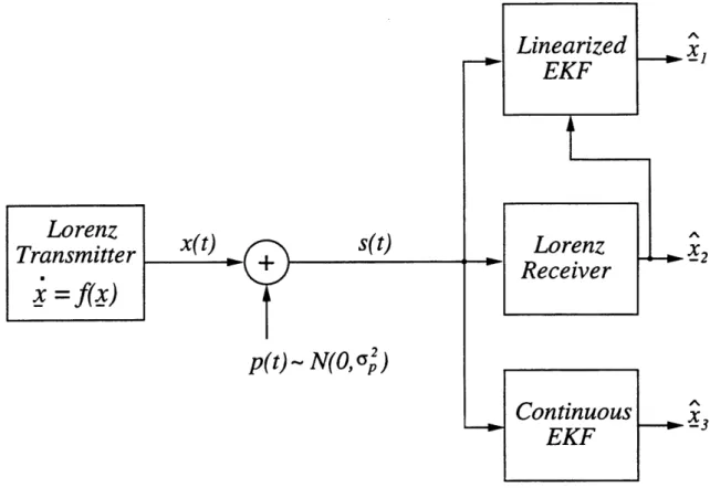
4.2 Performance Comparisons ... ... . 63
5 Robustness and Signal Recovery in a Synchronized Chaotic System 69 5.1 Experiments to Demonstrate Robustness and Signal Recovery ... . 70
5.1.1 Sensitivity of Synchronization to Additive White Noise ... . 72
5.1.2 Sensitivity of Synchronization to Additive Speech ... . . 73
5.2 Determining the Synchronization Error Moment Equations ... . 75
5.2.1 Approximate Approach ... 76
5.2.2 Exact Approach via Stochastic Calculus ... . 79
5.3 Development of an Approximate Synchronization Error Model ... . 87
5.3.1 Error Model Performance with Additive White Noise .... . 95
5.3.2 Error Model Performance with Additive Speech ... . 96
5.4 Summary ... 98
7
6 Synthesizing Self-Synchronizing Linear Feedback Chaotic Systems 103 6.1 x-Input/x-Output LFBCSs ...
6.1.1 Conditions for Global Self-Synchronization 6.1.2 Conditions for Global Stability ... 6.1.3 A Systematic Synthesis Procedure ... 6.1.4 Linear Stability Analysis ... 6.1.5 Numerical Example ... 6.2 z-Input/z-Output LFBCSs ...
6.2.1 Conditions for Global Self-Synchronization 6.2.2 Conditions for Global Stability ... 6.2.3 A Systematic Synthesis Procedure ... 6.2.4 Numerical Example ...
6.3 Summary ...
7 Synthesizing Self-Synchronizing Chaotic Arrays
7.1 Conditions for Global Self-Synchronization .... 7.2 Conditions for Global Stability ...
7.3 A Systematic Synthesis Procedure ... 7.4 Linear Stability Analysis ... 7.5 Numerical Example ... 7.6 Summary ... ... . . . 105 ... . . . 106 ... . . . 107 ... . . . 109 ... . . . 110 ... . . . 115 ... . . . 119 ... . . . 122 ... . . . 123 ... . . . 125 ... . . .. . .... 127 ... . . . 129 135 ... . . . 138 .. . .. .. 140 ... ... . . . 142 ... . . . 144 ... . . . 153 ... . . . 157
8 Synthesizing a General Class of Synchronizing Chaotic Systems
8.1 Conditions for Global Self-Synchronization ... 8.2 Conditions for Global Stability ...
8.3 A Systematic Synthesis Procedure ... 8.4 Linear Stability Analysis ... 8.5 Numerical Examples ...
8.5.1 The Lorenz System ...
8.5.2 A Four-Dimensional Synchronizing Chaotic System ... 8.5.3 A Five-Dimensional Synchronizing Chaotic System ... 8.6 Summary ...
9 Applications of Self-Synchronizing Chaotic Systems
9.1 Lorenz-Based Circuit Implementations ... 9.1.1 The Transmitter Circuit ... 9.1.2 The Receiver Circuit ... 9.2 Chaotic Signal Masking and Recovery ...
9.2.1 Concept ... 9.2.2 Circuit Experiment ...
9.2.3 Model-Based Signal Recovery ... 9.3 Chaotic Binary Communications ...
9.3.1 Concept ...
9.3.2 Synchronization Error Analysis and Detection .
185 ... . . . 186 ... . . . 186 ... . . . 190 ... . . . 194 ... . . . 195 ... . . . 196 ... . . . 197 ... . . . 202 ... . . . 202 ... . . . 203 8 161 163 166 168 170 171 171 173 176 183 _ _ __
9.3.3 Circuit Experiments ... 207
9.4 Summary ... 210
10 Conclusions and Suggestions for Future Research 213 10.1 Summary and Contributions . . . 213 10.2 Future Research Directions ... 215 A Linear Stability Analysis of z-Input/z-Output LFBCSs 217 B Lorenz Transmitter and Receiver Circuit Components 221
C Voltage-Controlled Resistor Circuit 223
9
List of Figures
2-1 Illustration'of Lyapunov's Direct Method ... 25
2-2 Positive Definite Functions . . . . . 26
2-3 A Trapping Region for the Lorenz Flow ... 28
2-4 Lyapunov Exponents of the Lorenz System ... 33
2-5 Lyapunov Dimension of the Lorenz System . ... 35
3-1 Decomposing a Chaotic System into Drive and Response Subsystems. 39 3-2 Lorenz Synchronizing Receiver Representations: (a) Decomposed Form. (b) Cascade Form. (c) Combined (3-D) Form ... 41
3-3 Synchronization of Transmitter and Receiver Signals in the Lorenz Sys-tem. (a) x(t) s. x,(t). (b) y(t) vs. y(t). (c) z(t) vs. z(t) . ... 43
3-4 SRS Tree for the Lorenz System.. . . . . 48
3-5 SRS Tree for the Double Scroll System ... 51
3-6 SRS Tree for the Rbssler System ... 52
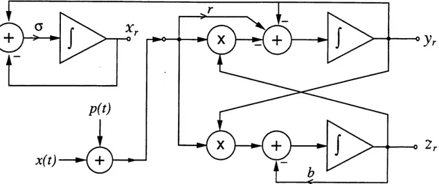
3-7 Block Diagram of the Lorenz Synchronizing Receiver. ... .. 56
4-1 Block Diagram of the Continuous EKF for the Lorenz System. .. 60
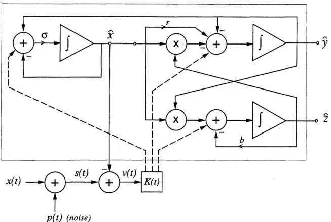
4-2 Block Diagram of the Linearized EKF ... ... . 61
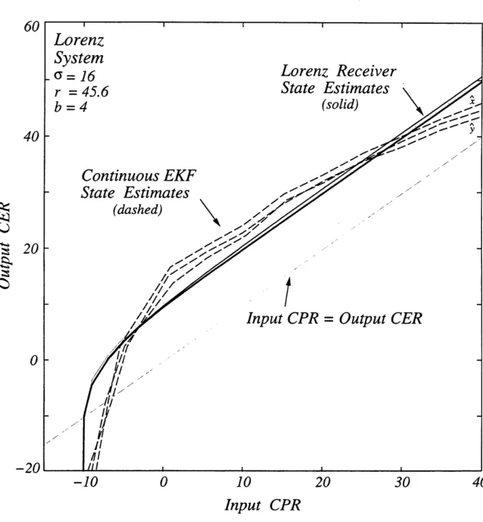
4-3 Numerical Experiment to Evaluate the Output CER vs. Input CPR. 65 4-4 Performance Comparison: Lorenz Receiver vs. Continuous EKF... 66
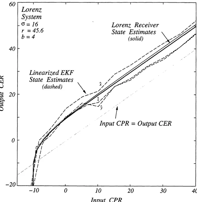
4-5 Performance Comparison: Lorenz Receiver vs. Linearized EKF .... 67
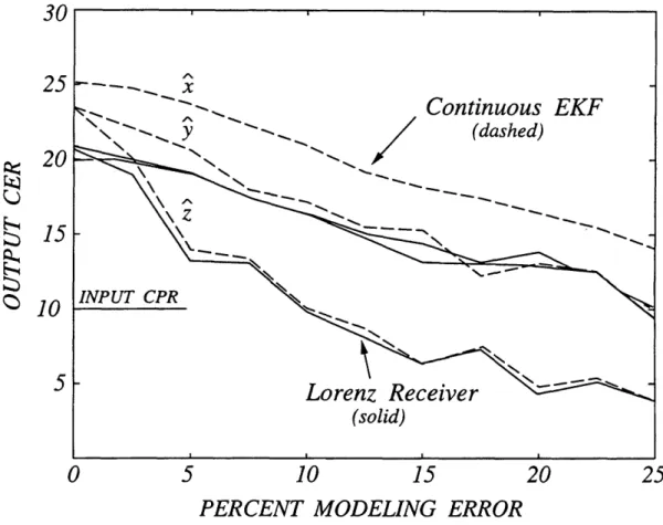
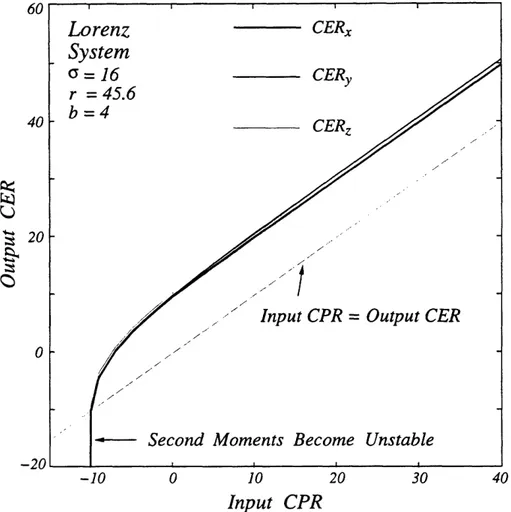
4-6 Sensitivity to Modeling Errors: Lorenz Receiver and Continuous EKF. 68 5-1 Output CER, CERy, and CERz vs. Input CPR for the Lorenz Syn-chronizing Receiver.. . . . . 73
5-2 True Power Spectra of the Error Signals: (a) E,(w). (b) Ey(w). (c) E (w ) . . . . 74
5-3 Power Spectra of x(t) and p(t) when the Perturbation is a Speech Signal. 75 5-4 Power Spectra of p(t) and Pl(t) when the Perturbation is a Speech Signal. 76 5-5 (a) Original Speech. (b) Received Signal. (c) Recovered Speech ... 77
5-6 Cascade System Representation of the Second Moment Equations... 82
5-7 Prediction of the Output CER From the Second Moment Equation.. 85
5-8 (a) Prediction of the Synchronization Error Variances From the Second
Moment Equation. (b) Synchronization Error Correlation Coefficients. 86
11
5-9 (a) Perturbation-to-Error Ratio vs. Lorenz System Parameter a
(In-put CPR=10 dB). (b) Perturbation-to-Error Ratio vs. Lorenz System
Parameter b (Input CPR=10 dB) ... 88
5-10 (a) A Sample Function of x(t). (b) A Sample Function of y(t). (c)
Power Spectra of x(t) and the Piecewise Constant Approximation of x(t). 91
5-11 Spread Spectrum Model of the Lorenz Error Dynamics ... . 92 5-12 Equivalent Linear Time-Invariant Model of the Lorenz Error Dynamics. 94 5-13 (a) Pole-Zero Plot for Hii(s). (b) Pole-Zero Plot for H12(s). (c)
Magnitude Response of Hx1(s) and H12(s). (d) Phase Response of
H
i
u(s) and H1 2(s) . . . . 955-14 True and Estimated Power Spectra of the Error Signals: (a) Ex(w).
(b) Ey(w). (c) Ez(w) . . . . . 96
5-15 Dynamical System Representation of the Message Recovery Process. 97
5-16 (a) Power Spectrum of p(t) and the True and Estimated Power
Spec-trum of e:(t). (b) Power SpecSpec-trum of p(t) and the True and Estimated
Power Spectrum of P3(t) ... . 99
5-17 Speech Waveforms: (a) True Recovered Message. (b) Recovered
Mes-sage using the Equivalent Linear Time-Invariant Model ... 100
6-1 Communicating with Linear Feedback Chaotic Systems ... 104
6-2 (a) Eigenfrequency Diagram for a 5-Dimensional x-input/x-output
LF-BCS. (b) Graphical Determination of the Bifurcation Parameter. (c)
Bifurcation Diagram ... 117
6-3 Lyapunov Exponents for a 5-Dimensional x-input/x-output LFBCS. . 118 6-4 Lyapunov Dimension for a 5-Dimensional x-input/x-output LFBCS. . 118 6-5 Chaotic Attractor for a 5-Dimensional x-input/x-output LFBCS.... 120 6-6 Self-Synchronization in a 5-Dimensional x-input/x-output LFBCS. . 121
6-7 (a) Eigenfrequency Diagram for a 5-Dimensional z-input/z-output LF-BCS. (b) Graphical Determination of the Bifurcation Parameter. (c)
Bifurcation Diagram . . . . . 128
6-8 Lyapunov Exponents for a 5-Dimensional z-input/z-output LFBCS. 130
6-9 Lyapunov Dimension for 5-Dimensional LFBCSs . ... 130
6-10 Chaotic Attractor for a 5-Dimensional z-input/z-output LFBCS ... . 131 6-11 Self-Synchronization in 5-Dimensional LFBCSs ... 132
7-1 Communicating with Chaotic Arrays ... 136
7-2 Stability Diagram for a 7-Dimensional Chaotic Array . ... 155
7-3 Lyapunov Exponents for a 7-Dimensional Chaotic Array . .... 156
7-4 Lyapunov Dimension for a 7-Dimensional Chaotic Array . ... 156
7-5 Self-Synchronization in a 7-Dimensional Chaotic Array . ... 158
8-1 Communicating with a General Class of Synchronizing Chaotic Systems. 162
8-2 Lyapunov Exponents for a 4-Dimensional Chaotic System ... . 175 8-3 Lyapunov Dimension for a 4-Dimensional Chaotic System ... 176 8-4 Chaotic Attractor Projections for a 4-Dimensional Chaotic System (r =
60) ... 177 12
8-5 Self-Synchronization in a 4-Dimensional Chaotic System ... 178
8-6 Lyapunov Exponents for a 5-Dimensional Chaotic System ... . 181
8-7 Lyapunov Dimension for a 5-Dimensional Chaotic System ... . 181
8-8 Chaotic Attractor Projections for a 5-Dimensional Chaotic System (r = 90) ... 182
8-9 Self-Synchronization in a 5-Dimensional Chaotic System ... 183
9-1 Lorenz-Based Chaotic Circuit ... 187
9-2 Circuit Data: (a) A sample function of u(t). (b) Averaged power trum of u(t). (c) A sample function of v(t). (d) Averaged power spec-trum of v(t) .. . . . . . . . 189
9-3 Circuit Data: (a) Chaotic attractor projected onto uv-plane. (b) Chaotic attractor projected onto uw-plane ... 190
9-4 Circuit Data: (a) Autocorrelation functions Ru(r) and R,v(r). (b) Probability density of u(t). (c) Probability density of v(t) ... 191
9-5 Circuit Data: Poincar6 section ... ... . 192
9-6 Circuit Data: First return map ... 192
9-7 Self-Synchronizing Receiver Circuit ... 193
9-8 Circuit Data: Synchronization of transmitter and receiver signals. . 194 9-9 Chaotic Signal Masking and Recovery System ... . 195
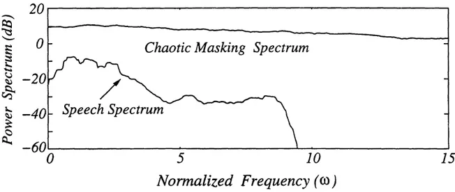
9-10 Circuit Data: Power spectra of u(t) and p(t) when the perturbation is a speech signal ... 196
9-11 Circuit Data: Power spectra of p(t) and P(t) when the perturbation is a speech signal ... .. . . . 197
9-12 (a) Recovered Speech (simulation) (b) Recovered Speech (circuit) ... . 198
9-13 Model-Based Signal Recovery ... 199
9-14 Communicating Binary-valued Bit Streams with Self-Synchronizing Chaotic Systems ... 203
9-15 Normalized Synchronization Error vs. Parameter Mismatch (percent). 206 9-16 Circuit Data: (a) Binary waveform used to modulate the b parameter of the Lorenz transmitter equations. (b) Averaged power spectrum of the drive signal with and without parameter modulation ... 209
9-17 Circuit Data: (a) Binary modulation waveform. (b) Synchronization error power. (c) Recovered binary waveform ... 211
C-1 Voltage-Controlled Resistor Circuit ... 224
13
14
Chapter 1
Introduction
For many years, there has been tremendous interest in the study of nonlinear dynam-ical systems that exhibit chaotic behavior. It is now well-understood that chaotic solutions of purely deterministic systems are an inherent feature of many nonlinear systems. Chaotic behavior has been reported in a broad range of scientific disciplines, including astronomy, biology, chemistry, ecology, engineering, and physics. Much of this research has focused on dissipative chaotic systems. Such systems are character-ized by limiting trajectories that are attracted to a region in state space that has zero volume and fractional dimension. Trajectories on this limiting set are locally unsta-ble, yet remain bounded within some region of state space. These sets are termed
strange attractors and exhibit a sensitive dependence on initial conditions in the sense
that any two arbitrarily close initial conditions will lead to trajectories that rapidly diverge. This inherent instability makes long term predictability of chaotic signals difficult because small uncertainties in the initial state will be exponentially amplified. Synchronization of dynamical systems possessing these properties would seem to be counter-intuitive. In 1990, however, it was discovered that a certain class of dissipative chaotic systems possess a self-synchronization property [1, 2, 3]. This property allowed two identical chaotic systems to synchronize when the second system was driven by the first. In certain communication contexts, the first system can be viewed as the transmitter and the second system as the receiver.
The phenomenon of synchronization has been of longstanding interest and studied 15
extensively. However, these studies had typically focused on the complex interactions among mutually coupled oscillator systems. The best known example is the motion of the earth and moon. Other more recent examples include: spatially distributed nonlinear systems such as coupled lasers [4], phase-locked loops [5], neural networks [6], and biological systems [7, 8]. There is, however, a fundamental difference between synchronization in mutually coupled systems and self-synchronizing systems. For the latter systems the coupling is one-way, i.e., only from the transmitter to the receiver.
The concepts of self-synchronization and chaos from purely deterministic systems suggest some potential applications - - one of the main motivating forces behind this thesis. Because chaotic signals are typically broadband, noise-like, and diffi-cult to predict, we have proposed their use in various contexts, e.g., as masks for information-bearing waveforms and as modulating waveforms in spread spectrum sys-tems [9, 10]. These proposed applications exploit the self-synchronization property to faithfully recover the information at the receiver. A major drawback to utilizing self-synchronizing chaotic systems in communication applications is that the analysis and synthesis of these systems is not well-understood due to their highly nonlinear nature. This thesis focuses on both of these critical areas.
With respect to analysis, we first develop a systematic approach for examining the self-synchronization properties of general nonlinear systems. Although this approach provides a valuable analysis tool, it does not provide much insight for understand-ing the mechanism underlyunderstand-ing the self-synchronization property. To overcome this limitation, we reformulate our analysis approach from the viewpoint of nonlinear stability theory. This approach enables us to identify an equivalence between self-synchronization in chaotic systems and asymptotically stable error dynamics between the transmitter and receiver systems. We then prove the global self-synchronization property of the Lorenz system and provide a clear mathematical framework for our subsequent analysis and synthesis techniques.
To utilize the Lorenz system in applications, it is important to examine the sen-sitivity of synchronization when a perturbation signal is added to the synchronizing drive signal. We establish an analogy between synchronization in chaotic systems,
16
nonlinear observers for deterministic systems, and state estimation in probabilistic systems. Then we show numerically that the performance of the Lorenz receiver as a nonlinear observer compares favorably with two well-known extended Kalman filter algorithms when the perturbation is white noise. The normalized error in syn-chronization of each state variable is significantly less than the normalized error in the drive signal, provided that the input chaos-to-perturbation ratio (CPR) is larger than some critical value. We use stochastic calculus to determine the exact first and second moments of the synchronization error signals when the perturbation is white noise. This analysis explains the observed threshold effect at low input CPRs. In ad-dition, the development of an equivalent linear time-invariant error model quantifies the sensitivity of synchronization in terms of the spectral characteristics of the per-turbation signal. This model explains why the synchronization is robust to wideband perturbations, and why low-level speech signals or other narrowband perturbations can be accurately recovered at the receiver even though the synchronization error is comparable in power to the message itself.
We next turn our attention to the synthesis problem. In [11], it was demon-strated that it is possible to create a five-dimensional chaotic system by augmenting the Lorenz system with additional states. That approach, however, involves consid-erable trial and error. In this thesis, we develop several systematic procedures for synthesizing new classes of high-dimensional dissipative chaotic systems that possess the self-synchronization property. The first class of systems that we introduce are referred to as linear feedback chaotic systems (LFBCSs). LFBCSs are composed of a low-dimensional chaotic system and a linear feedback system. We focus on LF-BCSs that utilize the Lorenz system as the chaotic system component and develop systematic synthesis procedures for this type of LFBCS. A second class of systems generalizes the LFBCS concept by allowing for multiple Lorenz systems and a linear system to be combined into a chaotic array. A systematic procedure for synthesizing this class of systems is also developed. The third class of systems represent a further generalization of these concepts; they eliminate the necessity of the linear system and, therefore, consist of an entirely nonlinear system. A systematic synthesis capability
17
--I--is provided which allows high-dimensional non-Lorenz self-synchronizing chaotic sys-tems to be designed. The synthesis techniques vary in the number of drive signals required for synchronization and the resulting complexity of the system dynamics. The flexibility afforded by the various synthesis techniques enhances the usefulness of synchronized chaotic systems for communications and signal processing.
Having a strong theoretical understanding of the concept of self-synchronization in chaotic systems, we next consider some applied aspects of these systems. First, we show that the Lorenz transmitter and receiver systems can be implemented as sim-ple analog circuits using commercially available hardware. The performance of these circuits is shown to be in excellent agreement with numerical and theoretical predic-tions. The desire to utilize the Lorenz circuits for private communications led us to develop two techniques for embedding an information-bearing waveform in the chaotic drive signal, and for recovering the information with the synchronizing receiver. With the first approach, we show that low-level speech signals can be privately transmitted and recovered with the receiver circuit. The second approach allows binary-valued bit streams to privately transmitted and recovered. While these two approaches do not represent the ultimate in privacy or practicality, they do mark an important starting point for the field.
1.1
Outline of the Thesis
The thesis is organized as follows. In Chapter 2, we summarize some relevant topics in nonlinear dynamics and chaos, and establish the notation used throughout the thesis. The emphasis of this summary is on the local stability analysis of equilibrium points, Lyapunov's direct method for examining global stability, and the concepts of Lyapunov exponents and attractor dimension for chaotic systems. Each of these topics plays a useful role throughout the thesis and the inclusion of this chapter makes the thesis self-contained. The reader can, however, omit this chapter without loss of continuity.
In Chapter 3, we generalize the ideas of chaotic system decomposition and
self-18
synchronization, and develop a systematic approach for determining all of the stable subsystems of general nonlinear systems. We then identify an equivalence between self-synchronization and stable error dynamics. This equivalence allows us to prove the global self-synchronization property of the Lorenz system and forms the basis for our analysis and synthesis techniques discussed in subsequent chapters.
In Chapter 4, we perform numerical experiments that quantify the sensitivity of synchronization in the Lorenz system when white noise is added to the drive signal. To calibrate the performance of the Lorenz receiver, we compare its performance against two well-known extended Kalman filter algorithms.
In Chapter 5, we perform a theoretical analysis of self-synchronization robustness and signal recovery in the Lorenz system. We use stochastic calculus to determine the exact first and second moments of the synchronization error signals when the drive signal is perturbed by white noise. An approximate analytical error model explains both the robustness of synchronization to wideband perturbations and why speech or other narrowband perturbations can be faithfully recovered at the receiver.
In Chapter 6, we synthesize a new class of chaotic systems called linear feedback chaotic systems (LFBCSs). The LFBCSs that we consider are composed of the Lorenz system and an N-dimensional linear feedback system. Our primary theoretical results include the development of self-synchronization and global stability conditions for this class of systems. Linear stability analysis leads to an approach for estimating the critical value of the bifurcation parameter at the onset of chaotic behavior. We also suggest a systematic procedure for synthesizing new LFBCSs.
In Chapter 7, we develop an approach for synthesizing chaotic arrays that consist of an arbitrary number of Lorenz oscillators and an N-dimensional linear system. The theoretical results include: (i) the development of self-synchronization conditions for this class of systems, (ii) the development of global stability conditions for this class of systems, and (iii) a systematic synthesis procedure.
In Chapter 8, we develop an approach for synthesizing a general class of
self-synchronizing chaotic systems. A systematic synthesis procedure is used to show that
the Lorenz system is only one member of a more general class of three-dimensional
19
I---chaotic systems which possess the self-synchronization property. To further illus-trate the simplicity and generality of the synthesis procedure, the design of higher dimensional chaotic systems is performed.
In Chapter 9, an analog circuit implementation of the Lorenz system is used to demonstrate two potential approaches to private communications based on synchro-nized chaotic signals and systems.
Chapter 10 summarizes the main contributions of this thesis and suggests some directions for future research.
20
Chapter 2
Nonlinear Dynamics and Chaos
In the main part of the thesis, we will need to utilize various well-known analysis techniques in nonlinear dynamics and chaos. In particular, local stability analysis, Lyapunov's direct method, and the concepts of Lyapunov exponents and attractor dimension play key roles throughout the thesis. This chapter summarizes each of these topics, with emphasis on nonlinear systems represented by a set of first-order ordinary differential equations. While the inclusion of this chapter makes the thesis self-contained, the reader can, however, omit this chapter without loss of continuity.
We begin by discussing the local stability analysis of nonlinear systems near the equilibrium points. This analysis proves useful in later chapters where it is necessary to find conditions on the system's parameters such that all of the equilibrium points will be unstable. We then discuss Lyapunov's direct method. This method is useful for examining the global stability of nonlinear systems and for determining trapping regions for a dissipative chaotic flow. Finally, we discuss some useful measures of chaotic behavior, in particular, the notions of Lyapunov exponents and attractor dimension. These measures are useful for confirming and comparing chaotic behavior for the various nonlinear systems that we consider.
21
2.1
Equilibrium Points and Local Stability
Throughout this thesis, we will focus our analysis and synthesis efforts on nonlinear systems which are representable by a set of ordinary differential equations of the form
=f(x), xERN . (2.1)
For simplicity, we will always assume that f(x) is a smooth function so that the basic existence-uniqueness theorems for ordinary differential equations apply to (2.1).
A typical starting point for the analysis of (2.1) is to determine the equilibrium (fixed) points and to perform a local stability analysis. The fixed points, x0, satisfy f(xo) = 0. Unfortunately, the determination of the zeros of a nonlinear function is of-ten not analytically tractable. There are, however, well-known numerical techniques, such as the Newton-Raphson method, which are well-suited to this problem.
For the purpose of discussion, let us assume that the fixed points of (2.1) have been determined. The ,behavior of solutions near x0 can be examined by linearizing
(2.1) at x0. The linearized system is given by
3 = Df(xo)6x, x E RN , (2.2)
where 5x = x- x and where Df = [fi/Dxj] is the system's Jacobian matrix. Because equation (2.2) is linear in 6x, the local stability of this system can be easily determined from the eigenvalues of the Jacobian matrix. Moreover, if Df(xo) has no zero or purely imaginary eigenvalues, then the local stability of solutions to (2.1) near xO is determined by the linearization [12]. This result is particularly useful in later chapters where it is necessary to determine the critical parameter values for which the fixed points of a nonlinear system undergo an abrupt change in stability. To illustrate these concepts, the fixed points of the chaotic Lorenz system are determined and a local stability analysis is performed.
The Lorenz equations, first introduced by E. N. Lorenz as a simplified model of
22
fluid convection [13], are given by
= U(y- -x)
p
= rx-y-xz (2.3)= xy-bz,
where a, r, and b are positive parameters. By varying r, the qualitative behavior of solutions to (2.3) can change abruptly. Abrupt changes in the qualitative behavior of a dynamical system are referred to as bifurcations and, in the case of the Lorenz system, r is commonly referred to as the bifurcation parameter. The critical values of r for which local bifurcations occur can be determined through linear stability analysis.
The first step is to determine the fixed points of the Lorenz system - - the origin is clearly a fixed point for all parameter values. Additionally, a pair of nontrivial fixed points exists when r > 1. The state space location of these fixed points is given by x = (iVb(r- 1), ±+b(r- 1), (r- 1)). The Jacobian matrix of the Lorenz system evaluated at the origin (xo = O) is given by
-a ar
0
Df(0) = r -1 0 0 0 -b
The eigenvalue at -b represents a stable mode since b > 0. The characteristic poly-nomial for the upper 2 x 2 block is given by
A2- (o + 1)A + o(1 -r) = 0.
The two roots of this characteristic polynomial are in the left-half plane for r < 1. For r > 1, one root is in the right-half plane and represents an unstable mode at the origin. Thus, r is a bifurcation parameter for the Lorenz system because a slight variation in r can abruptly alter the system's local stability.
The Jacobian matrix of the Lorenz system evaluated at the fixed point pair (x0 =
23
Xp) is given by
-a a 0
Df (xp) =
1
-1
- 1)
[b(
-
) ±Vb( - 1)
-
b
The characteristic polynomial of Df(xp) is given by
3 + (a + b + 1)A2 + b(a + r)A + 2ba(r - 1) = 0 . (2.4)
The critical value of r, when a root of (2.4) crosses from the left-half plane to the right-half plane, can be determined by applying the Routh-Hurwitz criterion. This critical value, r, is given by
rc (a +b+3) (2.5)
a-b-i
As r is varied, a local bifurcation occurs when r = r. For r > r, the fixed point pair is unstable. Thus, for r > max(l, rc) all fixed points of the Lorenz equations are unstable. Assuming that the trajectories remain bounded, either limit cycles or a chaotic attractor will exist. In Section 2.2, we utilize Lyapunov's direct method to show that all trajectories of the Lorenz system remain bounded for all positive parameter values. The interested reader may consult [12, 13, 14] for a more in-depth
analysis of the Lorenz equations.
2.2
Lyapunov's Direct Method
Lyapunov's direct method involves determining a family of closed curves (N = 2) or closed surfaces (N > 2) in state space such that the general behavior of nearby trajectories of a dynamical system can be examined. The best way to show how this works is by example.
y V(xy) Typical rajectory x /2/ k=3 F
Figure 2-1: Illustration of Lyapunov's Direct Method.
Example (Jordan and Smith [15])
In this example, consider the global stability of the origin for the system
X = -y-x, y = x-y3
To solve this problem, consider the family of closed curves V(x, y) = x2
+ y2 = k,
where k is a positive scalar. For each fixed k > 0, V(x, y) defines a circle enclosing the origin in the xy-plane as illustrated in figure 2-1. We wish to show that for any point on any of these circles, the state space trajectory through this point is directed toward the interior of the circle. If this property holds for all k > 0, then the origin is globally asymptotically stable. To show that this property holds, the total derivative of V(x, y) is evaluated along trajectories. Specifically,
dV(x(t),y(t)) aV V = (4 + 4)
dt -
&
94 + aySince V(x,y) is negative for all (x,y) 0, the trajectories move continuously to
smaller and smaller circles and eventually approach the origin. This shows that the origin is globally asymptotically stable.
In higher dimensional problems, V(x) is a positive definite scalar function of N components (x1,...,xN). By evaluating the total derivative of V(x), we can examine
25
V(x,y)
v(xy)
A
(a) (b)
Figure 2-2: Positive Definite Functions.
the behavior of trajectories in high-dimensional state spaces. Specifically, the total derivative of V(x) along trajectories is given by
dV(x(t)) N V
dt
=
E
-fi(x)
dt
i=1 x
where fi(x) is the component of the vector field associated with the ith state equation
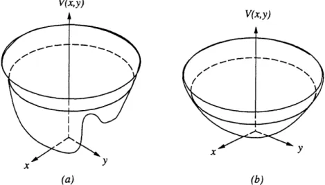
of the nonlinear system. If V(x) is a negative definite function, then the origin in state space is globally asymptotically stable. In general, positive definite functions may have multiple extrema as illustrated in figure 2-2(a). If, however, V1(x) is negative definite, then V(x) exhibits a single global minimum at the origin as illustrated in figure 2-2(b). Functions V(x) with this property are called Lyapunov functions. In later chapters, we will find Lyapunov functions particularly useful for examining the global stability of nonlinear systems.
In problems of a more general nature, it is often the case that stable fixed points do not exist, yet all trajectories remain bounded in state space. To examine the global behavior of trajectories in these systems, we consider quadratic positive definite functions of the form
1 V(x) = (x - C)TP(x - C) = k, (2.6) 2 26 x -y _I _
where P is a symmetric N x N positive definite matrix and k is a positive scalar. Geometrically, (2.6) represents a family of ellipsoids in state space with c defining the location of its center. Of particular importance for global stability analysis is the determination of a closed surface S for which V(x) = 0. If V(x) < 0 for all x outside S, then any ellipsoid T from the family (2.6) that contains S will suffice as a global trapping region for the N-dimensional flow. This means that all trajectories will eventually enter T and remain in T for all time thereafter. Finding a trapping region may be a difficult task; however, if one can be found then it can be used to prove that all trajectories remain bounded for all t > 0.
It is well-known that the Lorenz system provides an example of a nonlinear system for which an ellipsoidal trapping region can be analytically determined. As we show below, an ellipsoid from the family
1
V() = rx y2 +a(Z -2r)2) = k, k > o (2.7)
will determine a trapping region for the Lorenz flow for k sufficiently large. The total derivative of V(x) is given by
V(x) = -arx 2 - ay2 - a(z - r)2 + abr2
By setting V(x) = 0 and rearranging terms, we obtain
x
2 Y2 (z 2) = 1 . (2.8)-
+ +
~~~~~~~~~~~~(2.8)br br2 r2
Equation (2.8) represents an ellipsoid in state space. This ellipsoid plays the role of the closed surface S. Since V1 < 0 for all x outside of S, any ellipsoid T from the family (2.7) which contains S will suffice as a trapping region for the Lorenz flow. Figure 2-3 illustrates the trapping region T and the V(x) = 0 ellipsoid S.
Another key feature of the Lorenz flow is that it is highly dissipative. This can be shown by computing the divergence of the vector field for the Lorenz equations as
27
z
x
Figure 2-3: A Trapping Region for the Lorenz Flow. follows,
V x~ =~ ~~. A± ay ai- (o- + 1 + b)
V(x
=a + 5- +
a7
=Since the divergence is a negative constant, it follows that any volume in state space will contract exponentially fast [14]. The use of the divergence operator will be shown in Chapters 6-8 to be important for ensuring that our synthesis procedures produce chaotic systems which are dissipative.
In summary, linear stability analysis of the Lorenz system (Section 2.1) showed that for r > max(1, re) all of the fixed points are unstable and therefore the motion is non-trivial. Lyapunov's direct method was then used to illustrate that the Lorenz flow is confined to an ellipsoidal region in state space for all positive parameter values. Furthermore, invariant tori are not possible in the Lorenz system, because the diver-gence of the vector field is a negative constant. This property ensures that the Lorenz system is dissipative with exponentially fast volume contraction. This analysis alone does not guarantee the existence of chaotic behavior since the possibility for limit cycles exists. A dynamical system which behaves chaotically must exhibit a positive Lyapunov exponent. This issue is discussed in the next section.
28
2.3
Quantifying Chaotic Behavior
In this section, we discuss the concepts of Lyapunov exponents and attractor dimen-sion for dissipative chaotic systems. These concepts are used to measure and quantify the chaotic behavior of the various nonlinear systems that we consider in subsequent chapters of this thesis.
2.3.1
Lyapunov Exponents
Lyapunov exponents are the average exponential rates of divergence or convergence of nearby trajectories in a dynamical system. Positive Lyapunov exponents correspond to diverging trajectories in state space and set the time scale for reliable prediction of future states. Negative Lyapunov exponents correspond to converging trajectories in state space and set the time scale on which transient motion will decay [16]. In between these two extremes are the zero Lyapunov exponents which correspond to flow along the trajectory. If at least one Lyapunov exponent of a dynamical system is positive, then a volume element in state space will expand in some direction and nearby trajectories will diverge. The exponential expansion of a chaotic flow implies that diverging trajectories must experience a repeated folding process in order for the motion to remain bounded. Loosely speaking, each positive Lyapunov exponent reflects a "direction" for which the folding process takes place and trajectories become decorrelated. This dynamical behavior leads to a sensitive dependence on initial conditions and is a primary feature of every chaotic system.
Lyapunov exponents are most easily understood by considering a one-dimensional discrete-time map of the form
xn+1 = f(xn), x E R
Suppose that the initial state of this system is given by x = + xO, where xO represents an infinitesimal error in the true initial state Xo. The error in specifying
29
x, is given by
xn = xn.- xn = f () -f (xo)
Df'(xo)6xo
where f denotes the n-fold composition, f
_
f o ... o f. Applying the chain rule for differentiation we can writeDfn(xo) = Df(x._)Df (Xn-2) ... Df(xo)
and therefore, the average rate of exponential growth of 6xn is given by
JX" ~n-i
|xo
=
H
I Df(x)I
= eAn
i=O
The Lyapunov exponent, A, can then be expressed as 1 n-1
A = lim -loglDf(xi)I nooni=0
Lyapunov exponents can also be interpreted in information-theoretic terms [17]. Specifically, the positive exponents reflect the average rate at which predictive ability is lost, or equivalently, the average rate of information gained by observing the current state of the system. The well-known Henon map [18], for example, exhibits a positive exponent equal to 0.4. If the initial condition is known to a precision of 16 bits, then
the ability to predict beyond approximately 40 iterations is lost.
The concept of Lyapunov exponents also applies to continuous-time dynamical systems. To illustrate this, we denote the general solution of the dynamical system x(t) = f(x(t)), x E R, by x(t) = t(x(O)). Analogous to the discrete-time case, the initial state of the system is assumed to be given by x'(0) = x(0) + 6x(O), with the resulting error at time t given by
ax(t) = x'(t) - x(t) = Ot(x'(0))- Ot(x(0)) : Dt(x(0))6x(0)
30
By periodically sampling the linearized flow, Dot, the Lyapunov exponents for a continuous-time system can be defined as those of a discrete-time system generated by the mapping DebnT = Df '.
Several notable properties of continuous-time chaotic systems are:
* all continuous-time chaotic systems have at least one zero Lyapunov exponent corresponding to the direction tangent to the flow;
* the sum of the Lyapunov exponents is equal to the time averaged divergence of the vector field;
* any continuous-time dissipative chaotic system has at least one negative expo-nent, the sum of the exponents is negative, and the limiting trajectories evolve on an attracting set having zero volume in state space; and
* the minimum dimension of a continuous-time chaotic system is three.
Using a symbolic notation, the spectrum of Lyapunov exponents for a three-dimensional chaotic system has the unique representation (+, 0,-), whereas in four-dimensions there are three possible types, with representations given by (+, 0,-,-), (+, 0, 0,-) and (+, +, 0,-).
In dynamical systems with the state space dimension greater than one, the ex-istence and computation of Lyapunov exponents relies on the multiplicative ergodic theorem of Oseledec [19]. This theorem states that if a matrix product is defined as
Df
(x) = Df(f- 1(x)) Df(f(x))Df(x) ,then under some general ergodicity conditions, the following limit exists
lim -log ([Df'(x)]T[Df(x)]) = A ,
where A is a diagonal N x N matrix. Furthermore, the Lyapunov exponents corre-spond to the diagonal elements of A.
31
Unfortunately, a direct application of the multiplicative ergodic theorem is nu-merically unstable, especially when positive Lyapunov exponents exist. This diffi-culty has been overcome by the QR decomposition approach suggested by Eckmann and Ruelle [20], which is based on decomposing the matrix product Dfn(x) into triangular factors. Their approach begins by defining Df(x) = Q1R1, where Q is an orthogonal matrix and R1 is an upper triangular matrix. For j > 1, the matri-ces Ti(x) = Df(fi-l(x))Qj-l are sucmatri-cessively defined and decomposed according to TJ(x) = QjRj. It is straightforward to show that Dfn(x) = QnR ... R1. It can also
be shown that the diagonal elements Z) of the triangular matrix product Rn ... R obtained from this algorithm satisfy
lim 1logAn) = Ai,
n-+oonT
where Ai corresponds to the ith largest Lyapunov exponent.
The QR method provides a numerically stable approach for computing the Lya-punov exponents of a dynamical system defined by a set of state equations. Using the QR method, we show in figure 2-4 the computed Lyapunov exponents for the Lorenz system. For this case, the parameter values a = 16 and b = 4 were fixed, and the parameter r was varied over the range 20 < r < 100. Note that the onset of chaotic behavior occurs near r = 34 as evidenced by the existence of a positive Lyapunov exponent. The large negative exponent is due to the highly dissipative nature of the Lorenz chaotic attractor and, as expected, a zero Lyapunov exponent is also apparent. Note also that equation (2.5) determines that all of the fixed points will be unstable for r > 33.5. From figure 2-4, we see that this critical value closely
predicts when chaotic motion will occur.
2.3.2
Attractor Dimension
Long term chaotic motion in dissipative systems is confined to a strange attractor whose geometric structure is invariant to the evolution of the dynamics. Typically, a strange attractor is a fractal object and, consequently, there are many possible notions
32
5 Z -5 .o -10 Co -15 -20 -25
i~~~~~~~
I Stable-Fixed It Chaotic Region
Points
I
I
20 40 60 80 100
Bifurcation Parameter, r
Figure 2-4: Lyapunov Exponents of the Lorenz System.
of dimension for strange attractors. In this section, we discuss some well-known and widely accepted definitions of attractor dimension. We also discuss a simple relation-ship to Lyapunov exponents and provide a numerical example to further emphasize some useful aspects of these concepts.
Dissipative chaotic systems are typically ergodic. All initial conditions within the system's basin of attraction lead to a chaotic attractor in state space which can be associated with a time-invariant probability measure, p(x). Intuitively, the dimension of the chaotic attractor should reflect the amount of information required to specify a location on the attractor with a certain precision. This intuition is formalized by defining the information dimension, dimHp, of the chaotic attractor as
dimH = lim log p[Bx(e)]
E-4O log e
where p[Bx(e)] denotes the mass of the measure p contained in a ball of radius e, centered at the point x in state space [20, 21]. Information dimension is important
33
I I (
--- -I
from an experimental viewpoint because it is straightforward to estimate. The mass, p[Bx(e)], can be estimated by
M
p[Bx(e)] M U(e-x- xl) ,
where U(-) is the unit step function. In typical experiments, the state vectors x are estimated from a time delay embedding of an observed time series [22].
Information dimension will, in general, depend on the particular point x in state space being considered. Grassberger and Procaccia's approach [23] eliminates this dependence by defining the quantity
_ M M
C() M E E U(E-Ix- xjl)I
i=1 j=l
and then defining the correlation dimension, dimc p, as
dimcp = lim log C(e)
E-+0 log
In practice, one usually plots log C(e) as a function of log and then measures the slope of the curve to obtain an estimate of dimcp. It is often the case that dimHp and dimcp are approximately equal.
There is also a meaningful relationship between information dimension and Lya-punov exponents for chaotic systems [21, 24, 25]. If Al, ..., AN are the Lyapunov exponents of a chaotic system, then the Lyapunov dimension, dimLp, is defined as
dimLp = k + A +1 + k (2.9)
where k = max{i: Al + + Ai > O}. Equation (2.9) suggests that only the first k + 1 Lyapunov exponents are important for specifying the dimensionality of the chaotic attractor. Kaplan et al. [24, 25] conjecture that dimHp = dimLp in "almost" all cases. Clearly, if this is correct then equation (2.9) provides a straightforward way to estimate the attractor dimension when the dynamical equations of motion are known.
34
2.5 2 ;tIC 4 1.5
.
ZI .5 0 20 40 60 80 100 Bifurcation Parameter, rFigure 2-5: Lyapunov Dimension of the Lorenz System.
In figure 2-5, we show the computed Lyapunov dimension of the Lorenz attractor as the parameter r is varied over the range 20 < r < 100. Note that for r > 34, the Lyapunov dimension is nearly constant with an average value of approximately 2.06. This value is consistent with the correlation dimension of the Lorenz attractor given in [26]. Similar numerical experiments with the Henon, R6ssler, and double scroll [27] systems show a similar consistency. Since dimLp is relatively straightforward to determine, we will use this approach throughout the thesis to obtain meaningful estimates of the attractor dimension for the various chaotic systems that we consider.
35
36
Chapter 3
Self-Synchronization in Chaotic
Systems
The concept of chaotic synchronization is intriguing, and until recently, had not re-ceived much attention. It is now well-known that dissipative chaotic systems of a certain class possess a self-synchronization property. This property allows two iden-tical chaotic systems to synchronize when the second system is driven by the first. The ability to synchronize remote chaotic systems by linking them with a common drive signal suggests new and potentially interesting approaches to private communi-cations. Some applied aspects of synchronized chaotic systems will be discussed and demonstrated in Chapter 9.
Self-synchronization in chaotic systems is not well-understood due to the highly nonlinear nature of these systems. The analysis presented in this chapter provides a major step toward further understanding this remarkable property, and is organized as follows. In Section 3.1, we discuss the concept of chaotic system decomposition and demonstrate the self-synchronization property of the Lorenz system. In Section 3.2, we formalize this concept and develop a systematic approach for examining the self-synchronization properties of general nonlinear systems. In Section 3.3, we establish an equivalence between self-synchronization in chaotic systems and asymptotically stable error dynamics. We then use Lyapunov functions to provide an analytical explanation of self-synchronization in a class of chaotic systems.
37
-3.1
Decomposing Chaotic Systems into Drive and
Response Subsystems
In 1990, Pecora and Carroll [1, 2] reported that certain chaotic systems could be decomposed into drive and response subsystems that synchronize when coupled by a common drive signal. Specifically, they decomposed a nonlinear system of the form
x = f(x), x ERN ,
into subsystems, i.e., expressed it as
a
= D1(dl,d2), d RN- m (3.1)a2 = D2(dl,d2), d2 E Rm . (3.2)
This decomposition can be performed by simply partitioning the state variables into two groups, one associated with D1 and the other with D2. However, only certain partitions of the state variables will produce a stable D2 subsystem in the sense that all of the conditional Lyapunov exponents associated with D2 are negative. If a stable decomposition is achieved, then a stable response subsystem can be formed by duplicating D2 and replacing the state variables d2 by new state variables r. This leads to a response subsystem of the form
= D2(d1,r), r E Rm . (3.3)
Viewed as a single system, equations (3.1) and (3.2) can be interpreted as a transmit-ter or drive system with (3.3) forming a receiver or response subsystem that is driven by di. Figure 3-1 illustrates the approach.
In [1, 2], it was shown numerically that if the conditional Lyapunov exponents associated with D2 are all negative, then the state variables r will synchronize to the state variables d2. The term conditional is applied to emphasize that the dynamics of D2 depend on the drive variable d. In typical cases, an analytical determination of
38
I-- - - -I-- - - I
r(t)
LI
Drive System
Response Subsystem
d
1= D1 (d1,d2) = D2(d1,r)
d2- D2(d ,d2)
Figure 3-1: Decomposing a Chaotic System into Drive and Response Subsystems. the conditional Lyapunov exponents is not possible and numerical approaches, such as the QR decomposition method (Section 2.3), are necessary to calculate them.
The Lorenz system (2.3) provides an example of a chaotic system for which stable decompositions are possible. For example, a stable (yi, Z1) response subsystem can
be defined by
Y = rx(t) - Yi - x(t)z ()
Z = x(t)yl - bl
and a stable ( 2, z2) response subsystem by
x2 = a(y(t) - x2)
z2 = x2y(t) - bz2
Equations (3.4) and (3.5) represent dynamical response systems which are driven by the transmitter signals x(t) and y(t) respectively. It can be shown numerically that the conditional Lyapunov exponents of the (yi, zl) response subsystem are both negative and thus Y1 - yjl and Izl - z -+ 0 as t -+ oo [1, 3]. Also, the eigenvalues of the Jacobian matrix for the ( 2, z2) response subsystem are both negative and thus
Ix2 - x[ and z2 - z - 0 as t --+ oo.
The two response subsystems can be cascaded to regenerate the full-dimensional
39 _ __ --- I i I I I I I I I I I I
dynamics which are evolving at the transmitter [9, 10, 28, 29]. If the input signal to the (l,zl) subsystem is x(t), then the output y(t) can be used to drive the (x2, z2) subsystem. This subsequently generates a "new" (t) in addition to having
obtained, through synchronization, y(t) and z(t). It is also possible to regenerate the full-dimensional dynamics of the transmitter by reversing the order of the response subsystems and using y(t) as the drive signal. The advantage of using x(t) as the drive signal is that the two response subsystems given by equations (3.4) and (3.5) can be combined into a single system having a three-dimensional state space [30, 31, 32]. This produces a full-dimensional receiver system given by
Zr = (Yr -Xr)
Pr = rx(t) - Yr - (t)Zr (3.6)
z,
= (t)y, - bzrAn interesting feature of the receiver equations (3.6) is that they are algebraically similar to the transmitter equations (2.3), except that the drive signal x(t) replaces xr(t) in the second and third equations.
In figure 3-2(a), (b), and (c), we show the decomposed, cascade, and combined rep-resentations respectively, for a receiver system that can regenerate the full-dimensional dynamics of the Lorenz system. Note that the receiver depicted in figure 3-2(a) is four-dimensional and requires that two drive signals be communicated. The receiver depicted in figure 3-2(b) eliminates the need for two drive signals but is also four-dimensional. In an analog circuit implementation of the receiver systems, the state space dimension corresponds to the number of integrators and is, therefore, related to system complexity. The combined representation (figure 3-2(c)) requires the fewest integrators and is preferable in certain applications. For the remainder of the thesis, we will refer to the combined representation as the Lorenz receiver in light of the potential applications.
To illustrate the self-synchronization property of the Lorenz receiver, we show in figure 3-3(a) a comparison between the transmitter signal x(t) (dashed line) and the corresponding receiver signal xr (t) (solid line), when the receiver is initialized from the
Chaotic
Transmitter
Synchronizing
Receiver
x(t) (Drive Signal)
y(t) (Drive Signal)
y
z
x
z
x
z
(a) Decomposed Representation
x(t)
(b) Cascade Representation
XY
z
x(t) (Drive Signal) XrYr
Zrl(c) Combined Representation
Figure 3-2: Lorenz Synchronizing Receiver Representations: (a) Decomposed Form.
(b) Cascade Form. (c) Combined (3-D) Form.
41
I --- --. - -- --l --- , I _. _
-- Y
zero-state. Figures 3-3(b) and (c) show a similar comparison between the y(t) and z(t) transmitter and receiver signals, respectively. Synchronization is clearly rapid and maintained. Furthermore, the synchronization of the transmitter and receiver is global, i.e., the receiver can be initialized in any state and the synchronization still occurs. This important result will be proven analytically in Section 3.3.
The ability to decompose the Lorenz equations into cascading subsystems that regenerate the full-dimensional transmitter dynamics suggests an interesting approach for studying the self-synchronization properties of general nonlinear systems. This approach relies on determining the stable response subsystems for general nonlinear systems and is discussed in Section 3.2.
3.2
Determining the Stable Response Subsystems
for General Nonlinear Systems
The first step is to formalize the concepts of chaotic system decomposition and self-synchronization. We can then develop a systematic approach for determining all of the stable response subsystems for general nonlinear systems and show how to cascade these subsystems in an optimal way. While this analysis is presented using a continuous-time framework, the approach also applies to discrete-time systems.
The class of nonlinear systems that we consider is represented by a set of N first-order ordinary differential equations of the form
x = f1(x1, .. ,XN)
(3.7)
;N = fN(Xl, -..., XN)
The functions fl, ... , fN map RN -+ R1 and are assumed to be smooth. In our subse-quent analysis of chaotic system decomposition and self-synchronization, the following definition of driven subsystems will be useful.
42
x
y
Synchronizing
Receiver
x(t) (Drive Signal) Xr Yr ZrTransmitter Signal Receiver Signal
0 (a) 1 2 3 4 5 0 1 2 3 4 5 (b) 5 (c) 1 2 3 4
Time (s)
Figure 3-3: Synchronization of Transmitter and Receiver Signals
tern. (a) x(t) vs. xr(t). (b) y(t) vs. yr(t). (c) z(t) vs. zr(t).
in the Lorenz
Sys-43
Chaotic
Transmitter
y
-z
y(t)
80 z(t) 40 0 0 I-. _e ---X(t,
Definition 3.1 For any positive integer N, let JN be the set whose elements are the integers, 1, 2,..., N. Fix a proper subset j C JN. Let xj denote the set of state variables with indices that range over the elements of j. We say that a state xi, for
i E JN, drives a subsystem composed of states xj if and only if
j fj(xi,xj), i j
Applying Definition 3.1 to the Lorenz equations (2.3), we can conclude that:
* y drives the x subsystem, but that x does not drive the y subsystem because the equation for y also depends on the state z;
* neither x nor y alone drive the z subsystem by the same definition; and
* every two-dimensional subsystem of (2.3) satisfies Definition 3.1. Specifically, x drives the (y, z) subsystem, y drives the (x, z) subsystem, and z drives the (x, y) subsystem.
In fact, any system of the form (3.7) can be drive decomposed into subsystems, where each subsystem is driven by a single state variable. As discussed above, we see that exactly four driven subsystems exist for the Lorenz system. They are listed below.
1. x drives (y, z). 2. y drives (x, z). 3. z drives (x, y). 4. y drives x.
This approach to drive decomposition can be readily extended to N-dimensional systems. There are exactly N possible one-dimensional subsystems in the single drive variable case, i.e., one subsystem corresponding to each state variable. Equivalently,
44