by
JOEL TIDMORE JOHNSON
B.E.E. Elec. Eng., Georgia Inst. of Technology, Atlanta June 1991
Eng., Massachusetts Inst. of Technology, February 1993
Cambridge
Submitted to the Department of Electrical Engineering and Computer Science
in Partial Fulfillment of the Requirements for the Degree of DOCTOR OF PHILOSOPHY
at the
MASSACHUSETTS INSTITUTE OF TECHNOLOGY February 1996
©
Massachusetts Institute of Technology, 1996 All rights reservedSignature of A
uthor.
....
...
..---
---.
...
Depart of f ectric- Engineering and Computer Science February 1, 1996
Certified by
---Professor Jin Au Kong Thesis Supervisor
Accepted by
Frederic R. Morgenthaler
Chairn Depart ntal Committee on Graduate Students,' ASSAC•jUSETTS INS IU OF TECHNOLOG
APR 11
1996
LIBRARIES S.M. Elec.A
by
JOEL TIDMORE JOHNSON
Submitted to the Department of Electrical Engineering and Computer Science on February 1, 1996 in partial fulfillment of the requirements for the
Degree of Doctor of Philosophy
ABSTRACT
This thesis provides new computational models for electromagnetic surface scat-tering which allow large one and two dimensional problems to be considered through the use of efficient numerical algorithms and parallel computing techniques. This is in contrast with previous numerical studies that have been limited to relatively small surfaces rough in one dimension only. The new numerically exact models are applied to several problems of current interest, and allow studies of phenomena not predicted by any available analytical theories. In addition, comparisons are made with predic-tions of standard analytical models to obtain an assessment of their performance.
A one dimensional model for VHF propagation is the first numerical model considered. Comparisons with measurement data show the model to produce accu-rate results, and conclusively demonstaccu-rate the importance of terrain measurements in propagation predictions. Comparisons with approximate models allow their appro-priate regions of validity to be determined.
Polarimetric thermal emission from two dimensional periodic surfaces is stud-ied using an extended boundary condition (EBC) numerical solution. The model is applied to generate the only numerically exact results for two dimensional surface polarimetric thermal emission currently available, and demonstrates that properties of UB, the third Stokes emission parameter, remain similar to those observed previ-ously for one dimensional periodic surfaces. The response of UB to level of medium anisotropy is also investigated.
A Monte Carlo study of backscattering enhancement from two dimensional per-fectly conducting random rough surfaces follows, using a recently developed more efficient version of the method of moments which allows the large two dimensional surfaces investigated to be treated. Comparisons with bistatic scattering data from machine fabricated random surfaces taken at the University of Washington illustrate the first such validation of a two dimensional numerical scattering model to date. Backscattering enhancement is observed in both theoretical and experimental results, and theory and experiment are in good agreement.
Scattering from the surface of the ocean is studied using a two dimensional perfectly conducting surface Monte Carlo simulation. A simple power law spectrum model is chosen for the ocean surface, and variations with spectrum low frequency cutoffs are illustrated in the simulation. Both forward and back scattering from the ocean are considered, and comparisons are made with the standard composite surface model of ocean scattering which indicate appropriate choices of the "cutoff' wavenumber in the composite model. The validated composite surface theory is then used with more realistic ocean surface models to compare with measured ocean backscattering data.
Polarimetric thermal emission from the ocean is studied using a penetrable two dimensional surface Monte Carlo simulation. An extension to the standard penetrable surface method of moments is made to avoid greatly increasing the required number of surface unknowns for a highly lossy surface such as the ocean. Comparisons are made with the SPM and composite surface models for ocean scattering, and with available experimental data.
Thesis Supervisor: Professor Jin Au Kong
I wish to express my sincerest thanks to Prof. J. A. Kong, my thesis supervisor, for his guidance on the studies of this thesis, and for his advice and insights into many other aspects of electromagnetics research. His excellence in teaching has enabled me to obtain the skills necessary for this work, and the research group he has created has provided an enriching environment in which to develop research skills.
I also wish to express thanks to Dr. Robert T. Shin, for his unending enthu-siasm for surface scattering studies, which has provided great motivation, and for his willingness to address all technical issues in a clear and thorough fashion, which has helped immensely in handling technical issues along the way. I am grateful for the access I have had to Dr. Shin's technical expertise and to his solid grounding in real world problems and expectations. Thanks also to Prof. F. R. Morgenthaler for serving as a thesis reader, area exam member, and TA advisor.
I also wish to acknowledge collaborations with the University of Washington, particularly with Profs. Leung Tsang, Chi Chan, and Y. Kuga and with Kyung Pak. I appreciate the opportunity to have worked with Prof. Tsang while he was at MIT on sabbatical, and thank him for his willingness to collaborate in development and application of the SMFSIA approach. Collaborations with Groups 101 and 106 of Lincoln Laboratory are also acknowledged, with John Eidson of Group 106 providing
a great deal of assistance with the propagation simulations of this thesis.
In the EWT group at MIT, I would like to acknowledge all of the former mem-bers I have had the pleasure of interacting with, especially Drs. Ali Tassoudji, Murat Veysoglu, Simon Yueh, Son Nghiem, and Kevin Li. I would like to acknowledge the efforts of Dr. Eric Yang and Chih Chien Hsu in maintaining the group's computers,
and the help of Kit Lai as the group's secretary. Many technical discussions with Dr. K. H. Ding are also appreciated.
To all the current members of the EWT group, Chih Chien Hsu, Lifang Wang, Sean Shih, Yan Zhang, C. P. Yeang, Jerry Akerson, Fabio del Frate, and Nayon Tomsio, I wish you good luck in your continuing work and look forward to future collaborations. I appreciate the camaraderie we have shared, and acknowledge your
help in many areas.
Finally, I wish to thank my family for their continuing support through my graduate studies. This thesis is dedicated to my girlfriend Monica, who has shared every aspect of my life through the three years of this Ph.D. research with love, understanding, and thoughfulness. I look forward to our new future together.
The support of ONR contract N00014-92-J-4098, NASA contract 958461, and a National Science Foundation graduate fellowship are acknowledged. Sponsorship was also provided by the U.S. Air Force, under contract no. F19628-95-C-0002. Use of the Maui High Performance Computing Center is acknowledged, sponsored by Phillips Laboratory, Air Force Material Command under cooperative agreement F29601-93-2-001. The views and conclusions contained in this document are those of the author, and should not be interpreted as necessarily representing the official policies or en-dorsements, expressed or implied, of the US Air Force, Phillips Laboratory or the US Government.
Abstract
Acknowledgements
Dedication
1 Introduction
1.1 Background and Motivation ...
1.2 Basic Surface Scattering Formulation . . . .
1.2.1 Integral equations for surface scattering . . . .
1.2.2 Definition of field vectors ...
1.2.3 Definition of active remote sensing quantities .
1.2.4 Definition of passive remote sensing quantities
1.3 Review of Approximate Theories . . . .
1.3.1 Physical optics approximation . . . .
1.3.2 Small perturbation method . . . .
1.3.3 Two scale model ...
1.3.4 Other methods ...
1.4 Numerical Methods for Surface Scattering . . . .
21 . . . . 21 . . . . . 27 . . . . . 27 . . . . 32 . . . . . 33 . . . . . 37 . . . . . 39 . . . . . 40 . . . . . 43 . . . . 46 . . . . 48 . . . . . 48
1.4.1 Method of moments ...
1.4.2 Matrix equation solution methods ...
1.4.3 Computational facilities . . . . 1.5 Overview of Thesis ... . 50 . 53 * 55 . 56 2 VHF Propagation 2.1 Introduction ...
2.2 Review of Formulation and Numerical Method
2.3 Model Validation ...
2.4 Parallel Implementation . . . .
2.5 Comparison with Experimental Data . . . . .
2.6 Comparison with Other Propagation Models .
2.7 Conclusions ... 3 2-D 3.1 3.2 3.3 3.4 3.5 3.6
Periodic Surface Emission
Introduction ...
Formulation and Numerical Method .
Evaluation of Required Integrals ...
Model Validation . . . .
Pyramidal Surface Thermal Emission
Conclusions . . . .
4 Backscattering Enhancement
4.1 Introduction . . . .
4.2 Formulation and Numerical Method . . . .
CONTENTS 59 . . . . 59 . . . . . . 61 . . . . 67 . . . . . . 73 . . . . . . 76 . . . . . . 77 . . . . 88 91 91 96 103 111 117 126 129 129 132
4.3 4.4 4.5 Experimental Procedure . . . . Comparison of Results . . . . Conclusions ...
5 A Numerical Study of Ocean Scattering
5.1 Background and Motivation . . . .
5.1.1 Previous studies of ocean scattering .
5.2 Description of the Ocean Surface . . . .
5.2.1 Power law spectrum . . . .
5.2.2 Durden-Vesecky spectrum . . . .
5.2.3 Donelan-Banner-Jahne spectrum . .
5.3 Numerical Model for Ocean Scattering . . .
5.3.1 Canonical grid approach . . . .
5.3.2 Neumann iteration ...
5.3.3 Separation of coherent and incoherent
5.4 Approximate Models for Ocean Scattering .
5.5 Backscattering ... 139 141 148 153 153 terms
5.5.1 Backscattering from a power law spectrum ocean
5.5.2 Comparison with composite surface model . . . .
5.5.3 Comparison with Neumann iteration results . . .
5.6 Forward Scattering ...
5.6.1 Power law spectrum ...
5.7 Composite Surface Model for Non-power Law Spectra . .
5.8 Conclusions ... ... .... .. . . . . . 155 . . . . . 157 . . . . . 159 . . . . . 161 . . . . . 164 . . . . . 165 . . . . . 169 . . . . 172 . . . . 173 . . . . 174 . . . . 177 . . . . 179 . . . . . 188 . . . . . 196 . .. . .. . 200 . . . . 202 . . . . . 214 . . . . 221
5.9 Appendix - Physical Optics for Ocean Scattering ...
6 A Numerical Study of Ocean Thermal Emission
6.1 Introduction . .. ... . .. . .. . . .. . .. . . . .. .
6.2 Previous studies of ocean thermal emission . . . .
6.3 Approximate methods ...
6.4 Derivation of Penetrable Surface SMFSIA . . . .
6.4.1 Numerical impedance boundary condition (NIBC)
6.5 R esults . . . .
6.6 Sensitivity to Ocean Spectrum Model . . . .
6.7 Conclusions ... 7 Conclusions Bibliography
CONTENTS
223 227 .... 227 ... . 229 .... 231 ... . 234 ... . 239 .... 250 S. ... 259 .... 263 267 2731.1 Geometry of a canonical rough surface scattering problem ... 23
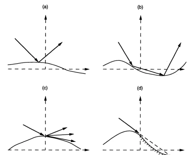
1.2 Mechanisms of rough surface scattering (a) Single scattering (b) Mul-tiple scattering (c) Diffraction (d) Shadowing . ... 24
1.3 Physical optics approach to surface scattering . ... 41
1.4 Small perturbation approach to surface scattering . ... 44
1.5 Composite surface approach to surface scattering . ... 47
2.1 Geometry of propagation problem . ... . 62
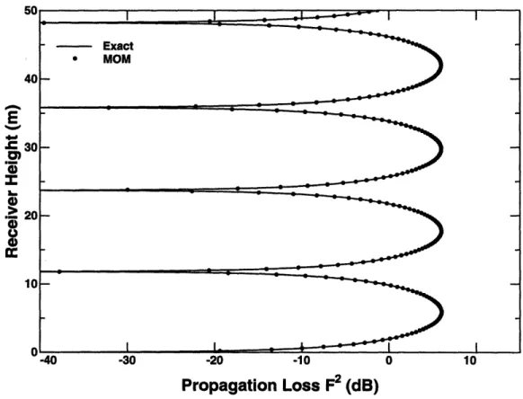
2.2 Excess one way propagation loss over a flat perfectly conducting plane - TE polarization: Comparison of MOM predictions with analytical solution . . . .. . 69
2.3 Wedge geometry for surface size tests . ... 70
2.4 Predicted excess one way propagation loss for perfectly conducting wedge - TE polarization: Comparison of results for varying total sur-face size . . . .. . 71
2.5 Predicted excess one way propagation loss for perfectly conducting wedge - TE polarization: Model predictions on each BMFSIA weak iteration . . . .. . 72
2.6 Predicted excess one way propagation loss for perfectly conducting wedge -TE and TM polarizations: Comparison of perfectly conducting and penetrable surfaces ... 74
LIST OF FIGURES
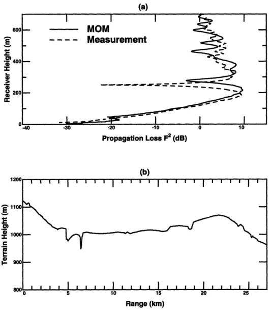
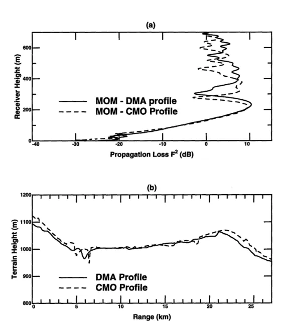
2.7 Comparison of MOM predictions with measurement data (a) excess
one way propagation loss (b) Beiseker N15 terrain profile ... .78
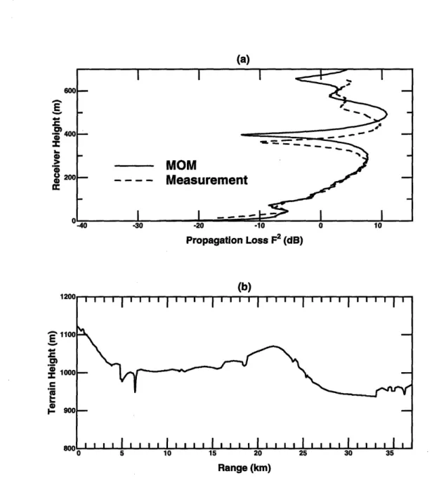
2.8 Comparison of MOM predictions with measurement data (a) excess one way propagation loss (b) Magrath NW27 terrain profile .... . 79
2.9 Comparison of MOM predictions with measurement data (a) excess one way propagation loss (b) Magrath NW37 terrain profile .... . 80
2.10 Variation of predictions with input terrain profile (a) excess one way propagation loss (b) Beiseker N15 terrain profiles . ... 81
2.11 Variation of predictions with input terrain profile (a) excess one way propagation loss (b) Magrath NW27 terrain profiles . ... 82
2.12 Variation of predictions with input terrain profile (a) excess one way propagation loss (b) Magrath NW37 terrain profiles . ... 83
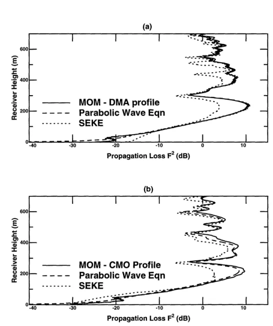
2.13 Comparison with analytic models - Beiseker N15 (a) DMA terrain pro-file (b) CMO terrain propro-file ... 85
2.14 Comparison with analytic models - Magrath NW27 (a) DMA terrain profile (b) CMO terrain profile ... 86
2.15 Comparison with analytic models - Magrath NW37 (a) DMA terrain profile (b) CMO terrain profile ... 87
3.1 Geometry of a one dimensional periodic surface . ... 93
3.2 Geometry of a two dimensional periodic surface . ... 94
3.3 Geometry of a two dimensional pyramidal surface . ... 103
3.4 Triangular grid in x - y plane for surface specification ... 104
3.5 Definition of surface plane through triangle . ... 106
3.6 Types of triangles in surface grid . ... . . . . 110
3.8 Comparison of induced currents on one dimensional wedge profile (a)
My (b) Jx (c) Mx (d) J, ... ... 116
3.9 Convergence of total reflected power with number of Fourier coefficients (a) Horizontal incidence (b) Vertical incidence (c) Horizontal power conservation (d) Vertical power conservation . ... 118
3.10 Predicted polarimetric brightness temperatures from a pyramidal sur-face: Variation with P, (a) TBh (b) TB, (c) UB (d) VB . . . . . . 121 3.11 Predicted polarimetric brightness temperatures from a pyramidal
sur-face: Variation with surface height (a) TBh (b) TBV (c) UB (d) VB . . 123 3.12 Predicted polarimetric brightness temperatures from a pyramidal
sur-face: Variation with polar angle (a) TBh (b) TB, (c) UB (d) VB . . . . 124
3.13 Predicted polarimetric brightness temperatures from a pyramidal sur-face: Variation with real dielectric constant (a) TBh (b) Ts, (c) UB (d)
VB . . . . . . 125
3.14 Predicted polarimetric brightness temperatures from a pyramidal sur-face: Variation with imaginary dielectric constant (a) TBh (b) TBv (c)
UB (d) VB ... ... .. 127
4.1 Comparison of Monte Carlo SMFSIA with experimental data. Surface area of 256 square wavelengths with an rms height of 1 wavelength and correlation length of 2 wavelengths. (a) ahh (b) ah (c) oh, (d) a,, . . 143
4.2 Comparison of Monte Carlo SMFSIA with experimental data. Surface area of 1024 square wavelengths with an rms height of 1 wavelength and correlation length of 2 wavelengths. (a) ahh (b) 0vh (C) Uhv (d) a,, 144
4.3 Comparison of Monte Carlo SMFSIA with varying sampling rates. Sur-face area of 1024 square wavelengths with an rms height of 1 wavelength and correlation length of 2 wavelengths. (a) ahh (b) avh (c) ahv (d) a,, 146
4.4 Comparison of Monte Carlo SMFSIA with experimental data. Surface area of 256 square wavelengths with an rms height of 1 wavelength and correlation length of 1.41 wavelengths. (a) ahh (b) avh (c) ah, (d) a,, 147
LIST OF FIGURES
4.5 Comparison of Monte Carlo SMFSIA with experimental data. Surface area of 256 square wavelengths with an rms height of 1 wavelength and correlation length of 3 wavelengths. (a) Uhh (b) avh (c) Uhv (d) avv . . 149 4.6 Comparison of Monte Carlo SMFSIA with experimental data. Surface
area of 1024 square wavelengths with an rms height of 1 wavelength and correlation length of 3 wavelengths. (a) 0
hh (b) Uah (C) 'hv (d) a,, 150 4.7 SMFSIA predictions of p (a) Real part of p for the simulations of Figure
4.1 (b) Imaginary part of p for Figure 4.7 (a) (c) Real part of p for the simulations of Figure 4.6 (d) Imaginary part of p for Figure 4.7 (c) . 151
5.1 Amplitude of Durden-Vesecky spectrum for 4 wind speeds ... 163
5.2 Amplitude of DBJ spectrum for 4 wind speeds ... 166
5.3 Comparison of Durden-Vesecky and DBJ curvature spectra ... 167
5.4 Comparison of MOM and SPM backscattering predictions for cutoff wavenumber kdl = 73.3: Convergence with respect to surface size . . . 179
5.5 Cutoff wavenumber kdl = 146.6, ka = 0.125 (a) Comparison of MOM and SPM backscattering predictions (b) Comparison of Monte Carlo and analytical PO backscattering predictions ... 182
5.6 Cutoff wavenumber kdl = 73.3, ka = 0.25 (a) Comparison of MOM and SPM backscattering predictions (b) Comparison of Monte Carlo and analytical PO backscattering predictions ... 183
5.7 Cutoff wavenumber kdl = 36.6, ka = 0.5 (a) Comparison of MOM and
SPM backscattering predictions (b) Comparison of Monte Carlo and analytical PO backscattering predictions ... . . . 184
5.8 Cutoff wavenumber kdl = 18.3, ka = 1.0 (a) Comparison of MOM and SPM backscattering predictions (b) Comparison of Monte Carlo and analytical PO backscattering predictions ... 185
5.9 Cutoff wavenumber kdl = 9.16, ka = 2.0 (a) Comparison of MOM and SPM backscattering predictions (b) Comparison of Monte Carlo and analytical PO backscattering predictions . ... 186
5.10 Cutoff wavenumber kdl = 4.58, ka = 4.0 (a) Comparison of MOM and SPM backscattering predictions (b) Comparison of Monte Carlo and analytical PO backscattering predictions . ... 187
5.11 Variation in vv backscatter cross sections with low frequency cutoff . 189
5.12 Variation in hh backscatter cross sections with low frequency cutoff . 190
5.13 Variation in hv backscatter cross sections with low frequency cutoff . 191
5.14 Comparison of PO and GO backscattering predictions using Kd = 2k 193
5.15 Comparison of PO and GO backscattering predictions using Kd = k/2 194
5.16 Comparison of MOM and composite surface model co-pol backscatter results . . . .. . 196
5.17 Comparison of MOM and SPM cross-pol backscatter results using a conductivity of l08 S-m in the SPM . ... 197
5.18 Comparison of MOM and single Neumann iteration backscattering pre-dictions, kdl = 9.16 ... 199
5.19 Cutoff wavenumber kdc = 4.58, ka = 4.0: Comparison of MOM, Monte Carlo PO, and analytical PO forward scatter co-pol cross sections for 60 degree incidence (a) 0, = 50 deg (b) 0, = 60 deg (c) 8, = 70 deg . 201
5.20 Cutoff wavenumber kdl = 9.16, ka = 2.0: Comparison of MOM, Monte Carlo PO, and analytical PO forward scatter co-pol cross sections for 60 degree incidence (a) 8, = 50 deg (b) 0, = 60 deg (c) 0, = 70 deg . 203
5.21 Cutoff wavenumber kdl = 18.32, ka = 1.0: Comparison of MOM, Monte Carlo PO, and analytical PO forward scatter co-pol cross sec-tions for 60 degree incidence (a) 0, = 50 deg (b) 0, = 60 deg (c) 0, = 70 deg . . . .. . 204
LIST OF FIGURES
5.22 Cutoff wavenumber kdl = 36.65, ka = 0.5: Comparison of MOM, Monte Carlo PO, and analytical PO forward scatter co-pol cross sec-tions for 60 degree incidence (a) 8, = 50 deg (b) 8, = 60 deg (c) 9, = 70
deg . . . .. .. . 205
5.23 Cutoff wavenumber kdl = 4.58, ka = 4.0: Comparison of MOM, Monte Carlo PO, and analytical PO forward scatter cross-pol cross sections for 60 degree incidence (a) 9, = 50 deg (b) 8, = 60 deg (c) 0, = 70 deg 206
5.24 Cutoff wavenumber kdl = 9.16, ka = 2.0: Comparison of MOM, Monte Carlo PO, and analytical PO forward scatter cross-pol cross sections for 60 degree incidence (a) 8, = 50 deg (b) 8, = 60 deg (c) 9, = 70 deg 207
5.25 Cutoff wavenumber kdl = 18.32, ka = 1.0: Comparison of MOM, Monte Carlo PO, and analytical PO forward scatter cross-pol cross sections for 60 degree incidence (a) 9, = 50 deg (b) 0, = 60 deg (c) 0
8 = 70 deg . . . 208
5.26 Cutoff wavenumber kdl = 36.65, ka = 0.5: Comparison of MOM,
Monte Carlo PO, and analytical PO forward scatter cross-pol cross sections for 60 degree incidence (a) O8 = 50 deg (b) O8 = 60 deg (c)
8, = 70 deg . . . 209
5.27 Comparison of MOM, Monte Carlo PO, and analytical PO forward scatter co-pol cross sections for 0 degree incidence with cutoff wavenum-ber kdl = 9.16, ko = 2.0 (a) 9, = -10 deg (b) 0, = 0 deg (c) 9, = 10 deg . . . .. .. . 210
5.28 Comparison of MOM, Monte Carlo PO, and analytical PO forward scatter co-pol cross sections for 30 degree incidence with cutoff wavenum-ber kdl = 9.16, ka = 2.0 (a) 0, = 20 deg (b) ,S = 30 deg (c) O8 = 40 deg . . . .. .. . 211
5.29 Variation in analytical PO forward scatter cross sections with low fre-quency cutoff at 60 degree incidence: co-pol cross sections (a) O, = 50 deg (b) 08 = 60 deg (c) 8, = 70 deg ... 212
5.30 Variation in analytical PO forward scatter cross sections with low frequency cutoff at 60 degree incidence: cross-pol cross sections (a)
0, = 50 deg (b) 9, = 60 deg (c) 0, = 70 deg ... 213
5.31 Comparison of analytical PO and GO forward scatter co-pol cross sections for 60 degree incidence with varying low frequency cutoffs,
Kd = k/4 (a) 9, = 50 deg (b) 0, = 60 deg (c) 8, = 70 deg ... 215
5.32 Comparison of analytical PO and GO forward scatter co-pol cross sections for 0 degree incidence with varying low frequency cutoffs,
Kd = k/2 (a) 0, = -10 deg (b) 0, = 0 deg (c) 0, = 10 deg ... 216
5.33 Composite surface model with DBJ spectrum: Comparison with AAFE experimental backscatter data (a) Wind speed 3.0 m/s (b) 6.5 m/s (c) 13.5 m/s (d) 23.6 m/s ... 218
5.34 Composite surface model with Durden-Vesecky spectrum: Comparison with AAFE experimental backscatter data (a) Wind speed 3.0 m/s (b) 6.5 m/s (c) 13.5 m/s (d) 23.6 m/s ... 220
5.35 GO co-pol forward scatter with Durden-Vesecky spectrum for incidence angle 60 degrees and Kd = k/4: Variation with wind speed (a) 0, = 50 deg (b) 08, = 60 deg (c) 0, = 70 deg ... 221
6.1 Comparison of SMFSIA/NIBC, Monte Carlo PO, SPM, and measured
(UB only) brightness temperatures: 14 GHz, nadir looking,
Durden-Vesecky spectrum, U19.5 = 10 m/s, surface temperature 283 K, kdl
-73.3, kdu = 1172.9, emissivity calculated as absorbed power (a) TBh (b) TBv (c) UBe ... 251 6.2 Comparison of SMFSIA/NIBC, Monte Carlo PO, SPM, and measured
brightness temperatures: 14 GHz, nadir looking, Durden-Vesecky spec-trum, U19.5 = 10 m/s, surface temperature 283 K, kdl = 73.3, kd,
-1172.9, emissivity calculated as one minus reflected power (a) TBh (b)
LIST OF FIGURES
6.3 Variation of SMFSIA/NIBC brightness temperatures with high fre-quency cutoff: 14 GHz, nadir looking, Durden-Vesecky spectrum, U19.5 =
10 m/s, surface temperature 283 K, kdl = 73.3, emissivity calculated as absorbed power (a) TBh (b) TBv (c) UB ... 255
6.4 Variation of SMFSIA/NIBC brightness temperatures with high fre-quency cutoff: 14 GHz, nadir looking, Durden-Vesecky spectrum, U19.5 =
10 m/s, surface temperature 283 K, kdl = 73.3, emissivity calculated
as one minus reflectivity (a) TBh (b) TBv (c) UB . . . . . . 256 6.5 Variation of SMFSIA/NIBC brightness temperatures with low
fre-quency cutoff: 14 GHz, nadir looking, Durden-Vesecky spectrum, U19.5 =
10 m/s, surface temperature 283 K, kdu = 1172.9, emissivity calculated as absorbed power (a) TBh (b) TBV (c) UB ... 257 6.6 Variation of SMFSIA/NIBC brightness temperatures with low
fre-quency cutoff: 14 GHz, nadir looking, Durden-Vesecky spectrum, U19.5 =
10 m/s, surface temperature 283 K, kdu = 1172.9, emissivity calculated as one minus reflectivity (a) TBh (b) TBs (c) UB . . . . . . 258 6.7 Variation of SPM brightness temperatures with high frequency cutoff:
14 GHz, nadir looking, Durden-Vesecky spectrum, U19.5 = 10 m/s,
surface temperature 283 K, kdl = 73.3 (a) TBh (b) TB, (c) UB . . . . . 261 6.8 Variation of SPM brightness temperatures with high frequency
cut-off: 14 GHz, nadir looking, DBJ spectrum, U19.5 = 10 m/s, surface
temperature 283 K, kd- = 73.3 (a) TBh (b) TBs (c) UB . . . . . . 262
6.9 Comparison of composite surface and SPM brightness temperatures: 14 GHz, nadir looking, U19.5 = 10 m/s, surface temperature 283 K, (a)
Introduction
1.1
Background and Motivation
Rough surface scattering plays an important role in many electromagnetic
applica-tions, including both active and passive remote sensing, wave propagation, and optical
and radar system design. Although approximate analytical techniques exist and work
well for certain types of surfaces, a general analytical solution to the rough surface
scattering problem remains to be discovered. At present, scattering from surfaces
whose properties render the analytical theories invalid can be accurately calculated
only through the use of numerical methods. Although numerical models are usually
too computationally complex for general use in most practical applications, they
pro-vide a valuable means for evaluating other approximate scattering models and for
decoupling uncertainties in the electromagnetic theories applied from uncertainties in
other areas, especially in specification of input surface properties. Additionally,
phys-ical insight gained from numerphys-ical solutions can potentially aid in the development of
future extended analytical theories. The ever increasing speed of moden computers
also motivates the development of numerical models, since practical problems can be
CHAPTER 1. INTRODUCTION
solved with more reasonable amounts of computational time than in the past, and
potentially with even less time in the future. The research of this thesis involves
nu-merically exact models for surface scattering and their application in remote sensing
and propagation problems.
A canonical rough surface scattering problem is illustrated in Figure 1.1, where
an incident time harmonic electromagnetic plane wave impinges upon a boundary, described by the function z = f(x), between two semi-infinite linear, homogeneous,
isotropic, and time-invariant media. Such LHITI materials are the only
electromag-netic media considered in this thesis. Determination of the resulting electromagelectromag-netic
fields in the space above and below the surface profile defines the problem to be
inves-tigated. The configuration of Figure 1.1 could represent a wave from a radar system
incident upon an ocean surface, for example, from which measurements of scattered
fields or power could potentially be used to determine physical properties of the
ocean. Alternatively, knowledge of the same scattered fields could be used to derive
brightness temperatures of an ocean surface observed by an airborne or spaceborne
radiometer. The configuration of Figure 1.1 could also model a laser beam incident
upon a optical grating, a VHF field propagating over Earth like terrain, a synthetic
aperture radar system observing soil moisture, or any number of other applications.
This wide range of possibilities motivates the study of rough surface scattering and
the desire for accurate and useful solutions to the rough surface scattering problem.
A well known solution to the problem of Figure 1.1 exists in the special case
z = 0 or z a linear function of x, for which the fields consist of a specularly reflected
z
Region 0
z=f(x)
24 CHAPTER 1. INTRODUCTION (a) (b) I I I I (c) (d) I I I I S -I--- ON
Figure 1.2: Mechanisms of rough surface scattering (a) Single scattering (b) Multiple scattering (c) Diffraction (d) Shadowing
solution of the boundary value problem for more general surface profiles is much more
difficult, given the many possible scattering mechanisms which can exist on a rough
surface. Heuristically, effects such a multiple scattering, diffraction, and shadowing, all illustrated in Figure 1.2, can exist singly or in combination, thereby making the
prediction of scattered fields very difficult. These scattering mechanisms can also
exist either locally (within an isolated region of the surface) or non-locally (coupling
distant regions of the surface), further complicating the physics involved.
I
Do-The above discussion considered surface profiles to be functions of coordinate
x alone. This type of surface is known in the literature as a one dimensional
(1-D) surface. More general surface profiles are functions of two spatial directions,
z = f(x, y), and are classified as two dimensional. Scattering behavior of rough
surfaces can be very different in the one and two dimensional cases, especially given
the decoupling of TE and TM polarizations associated with in-plane incidence in a
1-D problem. Due to the wider angular range over which scattered fields can exist
in a 2-D problem, scattered fields at specific in-plane angles are usually expected to
be lower than their 1-D counterparts. In addition, polarization coupling is inherent
in 2-D scattering and further reduces copolarized fields compared to 1-D. For reasons
to be discussed later, numerical models for 1-D surface scattering have received much
more study in the past. This thesis is concerned with both 1-D and 2-D numerical
models, but greater emphasis is placed upon the less studied 2-D case.
A final distinction exists between the random surface and deterministic surface
cases. Figure 1.1 illustrates the deterministic case, for which a fields are calculated for
a specified function describing the surface profile. However, since an exact functional
description of surfaces observed may not always be available, many applications
re-quire a random surface model. In the random surface case, the surface profile function
is modeled only in terms of its statistical properties as a stochastic process. Figure
1.1 could then be considered only to represent scattering from one realization of this
stochastic process, with an ensemble average of scattered fields or power over surface
realizations required to obtain statistical information about scattered field random
quanti-CHAPTER 1. INTRODUCTION
ties is clearly more useful in some instances, for example the ocean scattering problem
mentioned above. Information about scattered fields from one specific configuration
of the ocean surface is of little use since the surface itself changes both in time and
with observation location. However, statistical properties of these observations when
averaged over several observation times or locations are much less sensitive to such
variations.
Statistical description of the surface profile stochastic process involves
speci-fication of the joint probability density function for an infinite number of random
variables describing the height of the surface profile at individual values of coordinate
x. However, if the stochastic process is assumed to be a Gaussian process, meaning
that each of the individual surface height variables has a Gaussian height
distribu-tion, and to be stationary, meaning that its statistical properties are invariant with
respect to a shift of origin, a complete description of the process is given by
knowl-edge of its covariance function alone. Although realistic rough surface profiles are not
necessarily well described as stationary Gaussian stochastic processes, the immense
reduction in statistical complexity associated with such processes makes them highly
advantageous. Both deterministic and random surface profiles are considered in this
thesis, but only Gaussian process models are used in the random surface case.
The remaining sections of this chapter provide a brief overview of the theory
of rough surface scattering. In Section 1.2.1, integral equation formulations of
sur-face scattering are reviewed, and notations for scattered field, power, and brightness
temperatures to be used throughout the thesis are introduced. Three commonly used
review of numerical methods for electromagnetics follows in Section 1.4. Finally, an
overview of the chapters of the thesis is provided in Section 1.5.
1.2
Basic Surface Scattering Formulation
1.2.1
Integral equations for surface scattering
The standard dyadic Green's function formulation of Huygens' principle [1] states
that time harmonic fields of frequency w in a source-less volume V' bounded by a
surface S' can be related to the equivalent tangential electric and magnetic fields on
surface S' by
E(T) = /dS' {iw,~(f, T'). [' x H('·)] + V x [' x E()] (1.1)
7H(T) =
J
dS' -iweG(T, T'). [' x E(f')] + V x =G- [fi' x H(T)] (1.2)where n~ is a unit normal vector to surface S'. The above equation assumes the
medium inside volume V' to be a homogeneous, isotropic medium described by electric
permittivity e and magnetic permeability Iu, and a time dependency of e-wt is implied.
In addition, the observation point T is assumed to lie inside volume V' but not on
surface S'. The dyadic Green's function of the above equations is given by
v1
eikI|-F' (1.3)G
+
_(1.3)
k2
47rT
-
T'I
where I represents the unit dyadic and k is the electromagnetic wave number wVfLf.
28 CHAPTER 1. INTRODUCTION
in the integral equations, an infinitesimal spherical exclusion zone around the point
f is applied [2] and a limiting process yields
F(T)
=JdS'
{wp( '). [i' xH()+
xC[x (1.4)72
dS'
(-iwcG(:,
') ['
x
()] + V
x
.
['
x
H()]
(1.5)
where the integral f dS' is now performed as a principal value integration.For semi-infinite half spaces separated by a surface boundary as in Figure 1.1, a radiation condition argument can be applied which illustrates that the surface at
infinity does not contribute to the electromagnetic fields [1]. Thus, the above integral
equations state that knowledge of tangential electric and magnetic fields on the surface
profile bounding two semi-infinite half spaces determines fields throughout all of space.
For observation points on the surface profile, equations (1.4) and (1.5) constitute
coupled Fredholm integral equations of the second kind, whose solution yields the
unknown tangential fields which can then be used to determine fields throughout all
of space.
The problem of Figure 1.1 can be cast into an integral form by separately
considering the regions of space above and below the surface profile respectively. For
region 0 above the surface profile, a vector product of n with equations (1.4) and
(1.5) yields
2
x
Eo( x Ei-~nx + I x /dS' {iwI(tG , V). [i' xxHo(2
)=
Ax
•ine
+ A x dS' {-iweG(,
f).
[
x
T'
()]
+Vx
G.
[i'
x
H(')]}
(1.7)
where the contribution of the source fields, Einc and Hin, are now included. For
region 1 below the surface profile, the equations are
2
=
-,
.xfdS'
"
(iw•a,••,(T,T).
[i,'
x
H(f)]
+
Vx ~,
[i'
x
(e)]}
(1.8)
n x
H1
(T)
=
-
x/dS' {-
(, ').
x
2
+
Vx
G~, [n'
x
7H()]
(1.9)
where the incident field is no longer included since there is no source distribution
in the space below the surface profile, medium properties are modified to 61 and IL,
and the minus sign results from an assumed upward pointing definition for A'. Note
that the continuity of tangential electric and magnetic fields is implicit in the above
equations, since the same sources produce the total fields above and below the surface
profile. Equations (1.6-1.9) are the equations that will be solved for surface profile
tangential fields throughout this thesis. These four vector equations, however, are
not independent, as the magnetic field integral equations can be derived by taking a
curl of the electric field equations. Thus, use of one or a combination of equations
(1.6-1.7) along with one or a combination of equations (1.8-1.9) is required in order
CHAPTER 1. INTRODUCTION
this procedure to formulate the problem of scattering from a penetrable rough surface.
In the limit that the medium below the surface profile is perfectly
conduct-ing, tangential electric fields on the surface profile vanish and the relavent equations
become
0 = i x Ei,, + i x dS'
{iwmpG(Ti')
- [W'x H(f')]} (1.10)x Ho) - [(1.1)
2 x Hinc+ x f dS' Vx G. [' x H(')] (1.11)
known in the literature as the electric field integral equation (EFIE) and the magnetic
field integral equation (MFIE) respectively [3]. Either of these equations can be used
to solve the perfectly conducting halfspace medium problem, although there are some
important distinctions for thin conductors [4] which are not considered here. Since
the MFIE formulation usually results in a better conditioned numerical solution [3], it is applied in Chapters 4 and 5 of this thesis to the perfectly conducting surface
problem.
Another simplification of integral equations (1.6-1.9) is possible in the 1-D
sur-face case. The symmetries associated with a I-D problem allow knowledge of all field
components to be obtained from knowledge of the transverse electric and magnetic
field components, E, and Hy in Figure 1.1. Thus, solution of the surface scattering
problem requires knowledge of these field components alone on the surface profile.
Furthermore, for fields incident in the x - z plane alone, there is no coupling between
these TE and TM fields, so that two sets of three field components exist independently.
the vector Kirchhoff diffraction integrals,
= Einc + dS' (7') g, g (, 7') (1.12)
for the electric field in region 0 and similar equations for the electric and magnetic
fields in regions 0 and 1. Since fields in the I-D problem are determined by knowledge
of Ey and Hy alone, equations for the I-D problem become
Ey()= Eiy+ dS' Ey(7') g(,) g (, 7') Ey(?) (1.13)
H ) = Hinc + dS H, (') g( g, (7') ;,
H')
(1.14)2 _n On
E,2(( ') (, ') o
Sdr Eg(') )(OE-') (1.15)
2y( -; dS' Hy(T')Og) (' ) -gT (T T')
(
OHy(')
(1.16)2 On On
where continuity of tangential field components yields
OEy(7') __/E()')
n
a
a(OF
(1.17)
aH, (')
On = - \jOnOH(
)
(1(18')
(1.18)an
an
where a = 1 for the TE case (non-magnetic medium) and / = 1 for TM and in-planeE2 incidence is assumed. Furthermore, integration of these equations can be performed
32 CHAPTER 1. INTRODUCTION
function of
gj(p') Ho" - ) (1.19)
4
where Ho1 ) indicates the zeroth order Hankel function of the first kind and P reflects
the x - z plane distance as opposed to the three dimensional distance Y. One
di-mensional surfaces are studied in Chapter 2, and the above equations are used to
determine surface profile tangential field components.
1.2.2
Definition of field vectors
In this thesis, a spherical coordinate system will often be used to describe incident
and scattered field directions. For an incident electromagnetic plane wave, ýiei i,
propagating in direction ki, the following definitions are used:
kix = k sin Oi cos
qi
kiy = k sin Oi sinq i
kiz = -kcosOi (1.20)
where Oi refers to the incident polar angle, qi to the incident azimuthal angle. Two
unit vectors labeled hi and iji, for horizontal and vertical polarizations respectively,
orthogonal to this direction are defined as
hxki
h i
= < -~ sin Oi
+ ý cos Oi
ji = hi x ki = -x cos Oi cos Oi - ý cos 0i sin Oi - z sin Oi
Scattered fields are observed in the far field, where they consist of outward
propagating spherical waves, and scattered field propagation and polarization vectors
are defined as
ksx = k sin 0, cos 0,
ksy = k sin O0 sin 0,
ksz = k cos 0, (1.21)
xxk 8
hs = x = -_ sin
q,
+ ý cos o,8, = hS x ks = I cos 0, cos q, + ± cos 0, sin 4, - z sin O,
where 0s refers to the scattered polar angle, 0, to the scattered azimuthal angle. In
this notation, the forward scattering direction corresponds to 0, = Oi and 0, = 0i,
while backscattering is represented by either 0, = -Oi, /, = Oi or O, = 0i, 8, = 0i +7r.
1.2.3
Definition of active remote sensing quantities
Knowledge of the electric and magnetic fields throughout all of space implies a
com-plete solution of the problem of Figure 1.1 in the deterministic surface case.
Knowl-edge of the statistical properties of electric and magnetic field random variables is
pas-CHAPTER 1. INTRODUCTION
sive remote sensing measure only a small fraction of this information, and often report
scattered field amplitudes alone with no phase information. The specific terminology
used to describe scattered powers received in active remote sensing is reviewed in this
section.
Active remote sensing involves use of a radar system to transmit an incident
electromagnetic wave onto the medium under view and measurements of scattered
fields or power are reported. The power received in an ideal monostatic radar system
for a power transmitted Pt is given by the radar equation as
G2
A2
Pre = Pt (1.22)
(4r)3R4
where Gt represents the gain of the radar antenna, A is the wavelength, R the range
from transmitter to target, and a is a quantity describing the target known as the
radar cross section. Radar cross section a is defined as the area of an equivalent
isotropic radiator that would produce the same scattered power at the receiver as the
target, and is a function of frequency, incidence and scattered angles, polarization, and target physical properties. In the remote sensing of geophysical media, radar cross
sections are usually reported as normalized cross sections, aO, defined as ( where A
is the area illuminated by the transmitted antenna pattern. Only normalized radar
cross sections will be reported in this thesis, so the a notation will be used to indicate
A specific definition for the far-field normalized bistatic cross section is given by
cep (Os, 04, Si, q1) = lim 4irR2
fEaj
2 (1.23)R-*oo
AIE
') 12
where a, 3 = h, v represent the polarization of the scattered and incident waves
re-spectively, R is the range from the target to the observation point, E8 is the scattered
field amplitude, Ei is the amplitude of the field incident from direction (Oi, ij), and
A is the geometric area of the target. The above cross section is defined so that
integration of ahep + U, over all of space should give 4ir cos Oi for power conservation.
Monostatic radar systems measure the radar cross section only in the backscattering
direction. Both monostatic and bistatic radar system configurations are considered
in this thesis.
An alternate quantity 7, =, cos Oiis also commonly used and will be defined as
the normalized bistatic scattering coefficient in this thesis. This scattering coefficient
is normalized by the integration of ift Sinc, where Sinc is the Poynting flux density of
the incident wave, over the surface profile rather than SincA used for a. The factor
of cos Oi above results for plane wave incident fields.
For random surfaces, oa• is defined in terms of the ensemble average scattered
intensity as
47rR2
1Ea
|
2acp(0s, ¢s, 0i, 0i) = lim (1.24)
R-4oo
A E
2where the < -> notation above indicates an ensemble average over realizations of the
CHAPTER 1. INTRODUCTION
a coherent and incoherent part, defined as
4R 2 E > 12
Z' (0s, C s, 0i, 1i) = lim (1.25)
aaoo AE i)12
and
41rR2 < Eap >
12
OW (Os, IA, Ai, --lim < > (1.26)
aRoo
A|E
) 2
where the sum of the incoherent, u , and coherent, auo, parts is the same as (1.24).
This distinction will prove useful in Chapter 5 when comparing finite size surface
simulations with infinite size surface theories.
In polarimetric active remote sensing, measurements are made of correlations
between polarization amplitudes in addition to the power measurements discussed
above. The most commonly used additional parameter in polarimetric active remote
sensing is the Thh, a,, correlation parameter, p, defined as
p = lim R-Ioo <EhhE'v
hIEv
>I
(1.27)Measurement of rho implies a radar system capable of measuring phase differences
between received polarization amplitudes. The rho parameter has been shown useful
in identifying the similarity of hh and vv scattering mechanisms, since large values of
1.2.4
Definition of passive remote sensing quantities
In passive remote sensing, radiometers are used to measure thermal noise power
emit-ted from the object under view. The level of noise power measured is described in
terms of a brightness temperature, which is again a function of frequency, observation
angle, polarization, and medium properties. In addition, correlations between
hor-izontally and vertically polarized brightnesses are measured in polarimetric passive
remote sensing. The brightness temperature Stokes vector measured in polarimetric
passive remote sensing is defined as
(EhE*)
TB = 1- _ IE U (1.28)
C
U 7C 2Re(EEh)
V 2Im(EE) (1.28)
In the above equation, Eh and E, are the emitted electric fields received from the
horizontal and vertical polarization channels of the radiometer, 77 is the characteristic
impedance, and C = K/A2 with K denoting Boltzmann's constant, A the wavelength. The first two parameters of the brightness temperature Stokes vector correspond to
received powers for horizontal and vertical polarizations, respectively. The third
and fourth parameters correspond to the complex correlation between electric fields
received by the horizontal and vertical channels. These four parameters are labeled
TBh, TBv, UB, and VB respectively in this thesis.
It is shown in [5] that the third and fourth Stokes parameters may be related to
38 CHAPTER 1. INTRODUCTION
a right-hand-circularly polarized measurement (TBr) as follows:
UB = 2TBp -TBh -TBv (1.29)
VB = 2TBr -TBh -TBv (1.30)
Thus, to compute all four parameters of the Stokes vector, the brightness
temper-atures in horizontal, vertical, 45 degree linear, and right-hand-circular polarizations
are first calculated, and the above equations are used to obtain UB and VB.
The emissivity of an object is defined as the ratio of the brightness temperature
emitted by an object to its actual physical temperature, under the assumption that
the object is at a constant physical temperature, Tphys,
TBa = ea,(, ¢)Tphys
(1.31)
In the above equation, the subscript a refers to the polarization of the brightness
temperature, 0 to the polar observation angle, and ¢ to the azimuthal observation
angle. Through the principles of energy conservation and reciprocity, Kirchhoff's Law
relates this emissivity to the reflectivity of the surface [6]:
ea(0, ¢) = 1- ,ra(9, ) (1.32)
The reflectivity ra(9, €) for the given incident polarization a is defined as the
fraction of the power incident from direction (0, ¢) that is rescattered and can be
scattering angles in the upper hemisphere and summing the results of both orthogonal
scattering polarizations:
ra(0, ) = d' sin 9' j de'%Yba(0', 1'; 9, 0) (1.33)
In the expression of the bistatic scattering coefficient, (9, q) and (0', 0') represent
the incident and the scattered directions, respectively, and the subscripts a and b
represent the polarizations of the incident and the scattered waves, respectively.
Thus, to calculate the fully polarimetric emission vector, the bistatic scattering
coefficient for each of four polarizations is first calculated and integrated over the
upper hemisphere to obtain the reflectivity for that particular polarization.
Multipli-cation of the corresponding emissivity by the physical temperature of the object under
view yields the brightness temperature for this polarization. The fully polarimetric
brightness vector is then calculated as described previously.
1.3
Review of Approximate Theories
The solution of integral equations (1.6-1.9) is very difficult, given the arbitrary surface
profile S'. Analytical solutions to date have only been possible through the use of
approximations to reduce problem complexity. The approximations made are valid
for certain types of surfaces and scattering mechanisms, but neglect the contribution
of other scattering mechanisms and thus are not accurate in general. A variety of such
approximations have been studied in the literature for 1-D and 2-D, perfectly
CHAPTER 1. INTRODUCTION
theories are the physical optics approximation, or Kirchhoff approach, and the small
perturbation method. Each of these approximations are discussed in more detail
be-low, followed by brief sections on the composite surface model to be investigated in
Chapter 5 and on other surface scattering theories proposed in the literature.
1.3.1
Physical optics approximation
In the physical optics (PO) approximation, discussed in [8], tangential fields on the
surface profile are assumed to be the same as those that would exist on a plane tangent
to each point on the surface, as shown in Figure 1.3. Thus, given an incident field and
the height and first derivatives of the surface at a given point, the tangent plane can
be constructed, the incident field resolved into its locally TE and TM components,
and the total field calculated as the sum of the incident and reflected fields on the
interface. This procedure is repeated for every point of the surface profile to generate
tangential fields over the entire surface, which constitutes solution of equations
(1.6-1.9). The solution process is simple for a deterministic surface, and can be applied in
a Monte Carlo simulation for randomly rough surfaces. However, the simplicity of the
physical optics approximation also lends itself well to analytical averaging techniques
in the randomly rough case, especially for a Gaussian stochastic process.
For a perfectly conducting 2-D Gaussian process surface, the PO approximation
yields [6]
k2 1 + cos
Oi
+ cos 0 - sin Oi sinOs 27F cos Oi + cos 0,
Sdx'
Jdy'e"I
2CHAPTER 1. INTRODUCTION
for the normalized incoherent co-polarized bistatic cross section in the plane of
inci-dence q = 0, where kd = k- - ks, o2 is the variance of the rough surface, and C(x', y')
is the surface correlation function. A numerical evaluation of this integral will be used
in Chapter 5 to determine PO cross sections for an ocean surface model. However,
an examination of this equation reveals it to be an integration of a rapidly decaying
function in the large kad, case, making numerical evaluation of this integral difficult
for arbitrary C(x', y') and a. An analytical evaulation of the above integral is possible
for some specific correlation functions, including a Gaussian correlation function, and
results in an infinite series expression. A stationary phase integration method can
also be used in the large ckdz case, which results in the geometric optics (GO) limit
to equation (1.34) [8]: k2 1 + cos
Oi
+ cos 0 8 - sin Oi sinO0
2 7F cos Oi + cos 08 4- k 2 + k y2kexp2
2 C"(0) 2eC( (1.35)The GO expression above can be interpreted as the cross section of a flat plane
multiplied by the probability of obtaining a tilt angle such that the plane is normal
to the incident plane wave. The a2 C"(0) terms above can be shown to be equal to
the variance of the slope of the Gaussian stochastic process describing the surface.
Note that both the PO or GO solutions above predict no differences between
hh and vv results for perfectly conducting surfaces, and both also predict no cross
polarized fields in the backscattered direction. These results can be explained due to
shadow-ing and feature diffraction are also neglected, although attempts have been made to
include shadowing through the use of "shadowing functions" in the analytical
aver-aging procedure [10]. Physical optics solutions are therefore expected to be accurate
only when multiple scattering, shadowing, and diffraction do not contribute
signif-icantly to the final field solution. Thus, surfaces with fairly small slopes and large
radii of curvature, which limit multiple scattering effects, and near-forward
scatter-ing observations, which limit the effects of shadowscatter-ing, are required. No restrictions
are placed on overall surface rms variations however, as long as slopes remain small.
Studies of the validity of the PO and GO approximations have been performed for
1-D surfaces through comparison with numerical methods [29]-[33], primarily for
sur-faces with Gaussian correlation functions, and have quantified the above conditions
somewhat. However, comparisons for 2-D surfaces are much more limited.
1.3.2
Small perturbation method
A second approximate method for solving the rough surface scattering problem
in-volves a perturbation theory originally proposed in [7]. Field solutions are expanded
in perturbation series assuming that kizf(x', y'), kizif(x', y'), 9f W',) and 6f(x'"Y') are
small parameters, where k1zi is the 2 component of the transmitted wave vector.
Thus, the small perturbation method (SPM) requires that surface heights be much
smaller than a wavelength and small surface slopes in order for the series to
con-verge, as shown in Figure 1.4. The zeroth order solution consists of the specularly
reflected and trasmitted coherent waves, and the first order term contributes only to
CHAPTER 1. INTRODUCTION
z
Figure 1.4: Small perturbation approach to surface scattering
the coherent and incoherent fields, but are much more computationally complex.
For a perfectly conducting 2-D Gaussian process surface, the SPM
approxima-tion yields
Oab(Oi,
08)
=
16r
cos208,
cos2OifabW(kxs
-kxi,
kys
-kyi)
(1.36) for the normalized incoherent bistatic cross section in the plane of incidence to firstorder, where
= 1
(1 + sin2 0i)4
fAV
=
cos4 O0(1.37)
fhv = fvh=0. (1.38)
and W(k,, ky) is the power spectral density (or "spectrum") of the surface,
W(k,, k,) = 12
J
dx dy eikk ±+ikyy k 2C(x, y) (1.39)The SPM result above illustrates the "Bragg" scattering response in rough surface
scattering, which approximates the cross section as proportional to the spatial
fre-quency in the surface which would cause a periodic surface Floquet mode to
prop-agate in the observation direction. Note the polarization dependence of the above
cross sections which contrasts with the physical optics result obtained above. The
discrepancy between PO and SPM cross sections in the small surface height limit, for
which both theories should apply, has been addressed in the literature [28] and
elim-inated through an iteration of the PO result. Thus, the predicted SPM polarization
difference is accurate for small surface heights and slopes. Although the first order
solution predicts no depolarization in the plane of incidence, second order incoherent
fields yield a cross polarized contribution [34].
While the SPM is an exact perturbation solution, and therefore includes
contri-butions from all possible scattering mechanisms for surfaces for which it converges, it clearly is limited by the accuracy of its zeroth order solution. For surfaces where
significant scattering occurs, energy in the specularly reflected and transmitted waves