Digital Level Layers for Digital Curve Decomposition and Vectorization

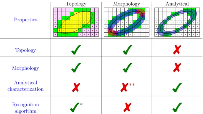
Having an analytical characterization has many advantages: it provides a way of verifying if a given set of digital points is a given digital circle or a subset of such a

Keywords Multigrid convergence · Digital estimator · Curvature · Shape Optimization · Image Segmentation.. This work has been partially funded by CoMeDiC ANR-15-CE40-0006

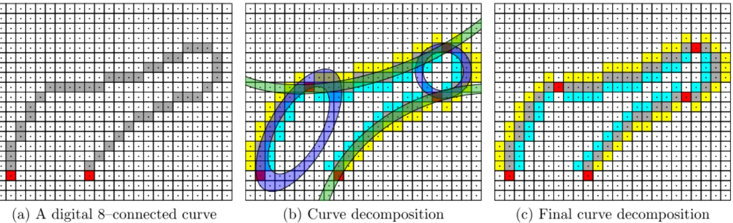
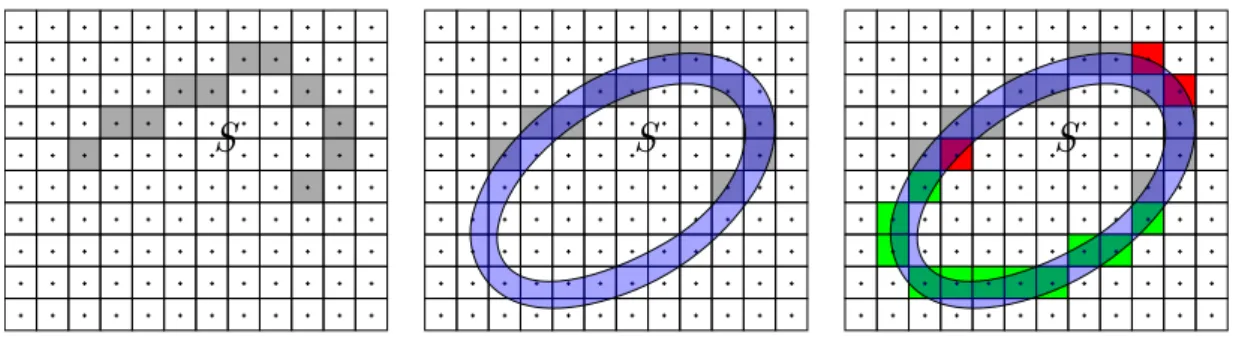
Based on a denition of the irregular isotheti digital straight lines, we present algorithms to re og- nize maximal irregular dis rete straight segments and to re onstru t

Because the digital economy can only work on the basis of confidence in the hardware, the quality of the information produced and the power and reliability

Following the spatial arrangement of variable and clause elements (see Figure 5), and the rules defined for the connections of negative and positive instances of variables

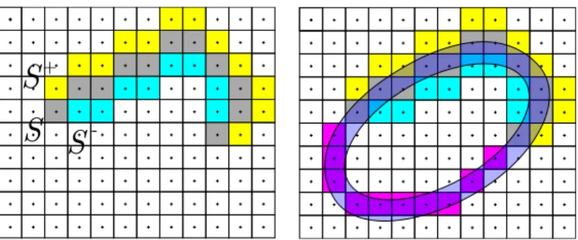
Due to definition 4, M and P are respectively the first upper and the last lower leaning points of the same MS, assumed without loss of generality to have points of

Definition 1 We call v-gadgets, c-gadgets and l-gadgets the digital objects encoding respectively variables, clauses and literals of a 3-SAT expression.. a b

L’archive ouverte pluridisciplinaire HAL, est destinée au dépôt et à la diffusion de documents scientifiques de niveau recherche, publiés ou non, émanant des