Variable time-step: A method for improving computational tractability for energy system models with long-term storage

(1)

HAL Id: hal-03100309

https://hal.archives-ouvertes.fr/hal-03100309

Submitted on 1 Jun 2021

HAL is a multi-disciplinary open access

archive for the deposit and dissemination of sci-entific research documents, whether they are pub-lished or not. The documents may come from teaching and research institutions in France or abroad, or from public or private research centers.

L’archive ouverte pluridisciplinaire HAL, est destinée au dépôt et à la diffusion de documents scientifiques de niveau recherche, publiés ou non, émanant des établissements d’enseignement et de recherche français ou étrangers, des laboratoires publics ou privés.

Variable time-step: A method for improving

computational tractability for energy system models

with long-term storage

Paul de Guibert, Behrang Shirizadeh, Philippe Quirion

To cite this version:

Paul de Guibert, Behrang Shirizadeh, Philippe Quirion. Variable time-step: A method for improving computational tractability for energy system models with long-term storage. Energy, Elsevier, 2020, 213, pp.119024. �10.1016/j.energy.2020.119024�. �hal-03100309�

(2)

1

Variable time-step: a method for improving computational tractability for

energy system models with long-term storage

Paul DE GUIBERT a, Behrang SHIRIZADEH a,b and Philippe QUIRION a*

Abstract

Optimizing an energy system model featuring a large proportion of variable (non-dispatchable) renewable energy requires a fine temporal resolution and a long period of weather data to provide robust results. Many models are optimized over a limited set of ‘representative’ periods (e.g. weeks) but this precludes a realistic representation of long-term energy storage.

To tackle this issue, we introduce a new method based on a variable time-step. Critical periods that may be important for dimensioning part of the electricity system are defined, during which we use an hourly temporal resolution. For the other periods, the temporal resolution is coarser.

This method brings very accurate results in terms of system cost, curtailment, storage losses and installed capacity, even though the optimization time is reduced by a factor of around 60. Results are less accurate for battery volume. We conclude that further research into this ‘variable time-step’ method would be worthwhile.

Keywords

: Energy system model; renewable energies; computational tractability; time series

aggregation; complexity reduction.

a_{CIRED-CNRS, 45 bis avenue de La Belle Gabrielle, 94736 Nogent sur Marne Cedex, France} b

TOTAL, GRP, R&D group, 2 place Jean Millier, 92078 Paris la Défense Cedex, France. * Corresponding author: quirion@centre-cired.fr, +33 (0)1 43 94 73 73

(3)

2

0. Introduction

Computation of optimized energy system models is very demanding in terms of calculation time and required memory. Hence modelers face a trade-off between, on the one hand, computational tractability and, on the other hand, comprehensiveness of the system modeled, broadness of the sensitivity analyses provided and accuracy of the results. This is especially true for energy systems featuring a high proportion of variable renewables (wind, solar photovoltaics and run-of-river hydropower), for at least three reasons.

First, a coarser-than-hourly temporal resolution lowers the model accuracy due to short-term variations in wind speed and solar radiation. Hence, most models feature an hourly resolution. This is sufficient for country-level modeling, but a coarser temporal resolution degrades model accuracy (Brown et al., 2018).

Second, inter-annual fluctuations in key weather variables are high (e.g. Collins et al. 2018; Zeyringer et al. 2018). This is true for wind and for temperature, which drives energy demand for heating and cooling. Optimization over several years is thus useful to check the reliability of an energy mix.

Third, due to annual cycles in wind, solar radiation and temperature, the cost-optimal solution often includes long-term energy storage, typically over several months (Schill and Zerrahn, 2018). Accounting for long-term storage requires the modeling of a continuous, long period of time, rather than defining ‘representative’ periods which may not ensure continuity of storage facility charge state (Pfenninger 2017, p.2).

Recent progress in energy system modeling includes, inter alia, sector coupling (e.g. Victoria et al., 2019), optimizing the location of renewable facilities over a large number of regions (e.g. Murray et al. 2020; Bramstoft et al. 2020), and analyzing the impact of climate change (e.g. Seljom et al. 2011; Ding et al. 2019), which requires optimization over many weather-years. While these developments are useful, they further increase calculation time and required memory. The issue is then to improve computational tractability in order to accommodate these improvements in model comprehensiveness without too great a loss of accuracy.

Some of the methods used to achieve this objective focus on aggregating time series, as in this paper. Hoffmann et al. (2020) provide an up-to-date, comprehensive review of these methods applied to energy system models. They classify the methods into two broad categories: (1) definition of typical

(4)

3

periods and (2) resolution variation. Clustering, which belongs to the first category, has gained particular attention in the literature. It consists of grouping together similar periods on the basis of a common characteristic. Clustering can be performed over representative hours as in Blanford et al. (2018) or over days as in Green et al. (2014). While clustering decreases calculation time, it does not maintain

chronological order, thus the state of charge and other hourly storage-related profiles cannot be modeled correctly using this method. Nahmmacher et al. (2016) suggest choosing several consecutive days within the representative periods. While this method can improve precision in dimensioning short-term storage technologies, it does not solve the above-mentioned problem of adequately representing long-term storage modeling.

The second method category, resolution variation, does not suffer from this problem since the continuity of time-steps is preserved, but the challenge is to maintain a fine enough resolution so that the specific characteristics of important hours are preserved. This cannot be achieved by uniform downsampling since, for example, the hour with the highest energy demand would be merged with contiguous hours, which by definition feature a lower demand.

Another family of resolution variation methods, called “segmentation” by Hoffmann et al. (2020), addresses this issue by varying the time resolution based on features of the supply and/or demand time-series. Mavrotas et al. (2008) use such a feature-based resolution variation algorithm to segment hourly time series to coarser time-steps for 3 seasons and 6 intra-day periods for heating, electricity and cooling loads. Samsatli and Samsatli (2015) and Pineda et al. (2018) also apply this type of method. The limitation of these methods is that even for a given season and intra-day period (e.g. evenings in winter), there may be a significant heterogeneity, for example in energy demand, which is not accounted for.

The strategy we propose in order to overcome these limitations is to maintain an hourly temporal resolution for the ‘most important’ hours, while adopting a coarser resolution for the rest of the

optimization period. To use the same vocabulary as Hoffmann et al. (2020), we develop a feature-based method to decrease the number of time-steps by hierarchical segmentation: we first define critical periods represented as hourly time-steps, then we apply a daily downsampling. As in the other resolution variation methods, the chronological order is retained.

This strategy has been inspired by another computationally demanding scientific domain: atmospheric modeling. Many atmosphere models feature a finer spatial definition over the region of interest to

(5)

4

modelers, e.g. Europe for many applications of the models developed in this continent (e.g. Hourdin et al., 2013 for LMDZ, the atmospheric part of the IPSL coupled climate model).

The main difficulty is choosing the ‘most important’ hours, hence in this article we propose a method to achieve this and we test the performance of this ‘variable time-step’ approach in terms of model accuracy and calculation time. We apply the method to two national energy system models,

EOLES_elecRES (Shirizadeh et al., 2019) and DIETER (Zerrahn and Schill, 2015), which have previously been implemented at an hourly resolution.

The first section below introduces the ‘variable time-step’ method. Section 2 describes the two energy system models within their specific cases, to which the method is applied, section 3 presents the results, first for a central cost scenario and second for alternative cost scenarios. Section 4 presents the

discussion and conclusion.

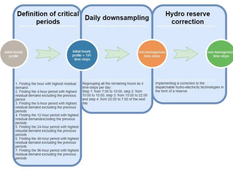
1. The ‘variable time-step’ method

Our ‘Variable time-step’ method can be defined as follows: all the hours of the considered period (one or several weather-years) are included in the optimization in chronological order but some consecutive hours are grouped into single time-steps, some of which are therefore longer than others. The idea is to maintain an hourly resolution for hours which may matter for dimensioning part of the electricity system (production or storage installations) and to group the other hours into single time-steps.

1.1. Definition of critical periods

We select the hours to be grouped on the basis of residual demand variation. Residual demand is the difference between demand and generation by non-dispatchable technologies (wind, solar and river-based hydro). For example, during a given night, consumption is relatively constant and solar power production is zero, so, provided that the wind blows relatively constantly, there is little variation in residual demand. These night hours can therefore be grouped into a single time-step without much loss of accuracy. Equation (1) shows the mathematical definition of residual demand:

𝑑_ℎ𝑟𝑒𝑠𝑖𝑑𝑢𝑎𝑙 _{= 𝑑}

ℎ− ∑𝑣𝑟𝑒𝐺𝑣𝑟𝑒,ℎ (1)

Where 𝑑ℎ𝑟𝑒𝑠𝑖𝑑𝑢𝑎𝑙 is the residual demand at hour ℎ, 𝑑ℎ is the electricity demand at hour ℎ and 𝐺𝑣𝑟𝑒,ℎ is the hourly power production from variable renewable energy source 𝑣𝑟𝑒 (non-dispatchable production).

(6)

5

To set the duration of the critical periods (those which require an hourly resolution) we chose several periods to cover various difficult situations that must be overcome by the power system. The hours with the highest residual demand are of great importance since the installed capacity should be sufficient to satisfy peak residual demand. Li-Ion batteries for stationary applications in hourly dispatch can be used for both power reliability and power quality, and the intersection between these two applications is a four-hour period (Schmidt et al, 2019); thus, a volume-to-power ratio of four hours (i.e. they can be fully charged and discharged in four hours in nominal power). We therefore chose the four-hour period with the highest residual load as a second critical period duration.

The longest period should be chosen in such a way that short-term and mid-term storage options (batteries and PHS) are modelled correctly. An analysis on the full discharge time of the pumped hydro storage (mid-term storage) technology is necessary to define the longest period. According to Shirizadeh et al. (2019) discharge time of PHS plants rarely exceeds four days, therefore, we consider the longest period to be 96 hours. This analysis for the case studied by Shirizadeh et al. (2019) is presented in appendix 1.

Since adding a limited number of time-steps does not significantly change the solution time, we added six-hour, twelve-hour, one-day and two-day periods in between the previously mentioned critical periods. The critical periods are found by the equations (2) to (8):

ℎ1∈ 𝐻 = {1,2, … ,8760}; 𝑑_ℎ𝑟𝑒𝑠𝑖𝑑𝑢𝑎𝑙₁ _{= max} ℎ∈𝐻𝑑ℎ𝑟𝑒𝑠𝑖𝑑𝑢𝑎𝑙 (2) 𝐻₂= {ℎ, ℎ + 1, ℎ + 2, ℎ + 3} ⊂ 𝐻 − ℎ₁ ; ∑ 𝑑_ℎ𝑟𝑒𝑠𝑖𝑑𝑢𝑎𝑙 ℎ∈𝐻2 = max_𝐻−ℎ 1 ∑ 𝑑_ℎ𝑟𝑒𝑠𝑖𝑑𝑢𝑎𝑙 ℎ∈𝐻2 (3) 𝐻₃= {ℎ, ℎ + 1, … , ℎ + 5 } ⊂ 𝐻 − 𝐻₂− ℎ₁ ; ∑ 𝑑_ℎ𝑟𝑒𝑠𝑖𝑑𝑢𝑎𝑙 ℎ∈𝐻3 = max_𝐻−𝐻 2−ℎ1 ∑ 𝑑_ℎ𝑟𝑒𝑠𝑖𝑑𝑢𝑎𝑙 ℎ∈𝐻3 (4) 𝐻₄= {ℎ, ℎ + 1, … , ℎ + 11 } ⊂ 𝐻 − 𝐻₂− 𝐻₃− ℎ₁; ∑ 𝑑_ℎ𝑟𝑒𝑠𝑖𝑑𝑢𝑎𝑙 ℎ∈𝐻4 = _𝐻−𝐻max 2−𝐻3−ℎ1 ∑ 𝑑_ℎ𝑟𝑒𝑠𝑖𝑑𝑢𝑎𝑙 ℎ∈𝐻4 (5) 𝐻₅= {ℎ, ℎ + 1, … , ℎ + 23 } ⊂ 𝐻 − 𝐻₂− 𝐻₃− 𝐻₄− ℎ₁; ∑ 𝑑_ℎ𝑟𝑒𝑠𝑖𝑑𝑢𝑎𝑙 ℎ∈𝐻5 = _𝐻−𝐻 max 2−𝐻3−𝐻4−ℎ1 ∑ 𝑑_ℎ𝑟𝑒𝑠𝑖𝑑𝑢𝑎𝑙 ℎ∈𝐻5 (6)

(7)

6 𝐻₆= {ℎ, ℎ + 1, … , ℎ + 47 } ⊂ 𝐻 − 𝐻₂− 𝐻₃− 𝐻₄− 𝐻₅− ℎ₁; ∑ 𝑑_ℎ𝑟𝑒𝑠𝑖𝑑𝑢𝑎𝑙 ℎ∈𝐻6 = _𝐻−𝐻 max 2−𝐻3−𝐻4−𝐻5−ℎ1 ∑ 𝑑_ℎ𝑟𝑒𝑠𝑖𝑑𝑢𝑎𝑙 ℎ∈𝐻6 (7) 𝐻₇= {ℎ, ℎ + 1, … , ℎ + 95 } ⊂ 𝐻 − 𝐻₂− 𝐻₃− 𝐻₄− 𝐻₅− 𝐻₇− ℎ₁; ∑ 𝑑_ℎ𝑟𝑒𝑠𝑖𝑑𝑢𝑎𝑙 ℎ∈𝐻6 = _𝐻−𝐻 max 2−𝐻3−𝐻4−𝐻5−𝐻7−ℎ1 ∑ 𝑑_ℎ𝑟𝑒𝑠𝑖𝑑𝑢𝑎𝑙 ℎ∈𝐻6 (8) 1.2. Daily sub-sampling

The next step is to group the remaining hours in a coherent way. This daily sub-sampling depends on the studied case. We define four main daily time-slices, depending on the availability of solar irradiation and daily electricity demand:

a) Morning: a transition period during which non-dispatchable generation rises steeply.

b) Noon: the period with the maximum excess non-dispatchable generation, which determines the required storage volume.

c) Evening: the period with the highest residual demand, resulting in massive use of dispatchable technologies.

d) Night: a period during which residual demand is low, resulting in little use of dispatchable technologies, while storage technologies can be charged during this period.

These four periods can vary among different geographical locations and different life-styles. For our two case studies, these four time-slices are chosen:

a) Morning: 7 am to 10 am. b) Noon: 10 am to 3 pm. c) Evening: 3 pm to 10 pm.

d) Night: 10 pm to 7 am of the day after.

1.3. Hydro reserve correction

During the evening period, residual demand is high. The model satisfies this demand by using batteries, dispatchable hydraulic power, biogas and gas from methanation. However, a problem with the method described above is that it allows the saturation of hydraulic power to be bypassed when it occurs for only a short time. For example, in the model with a variable time-step, during the period from 3 pm to 10 pm hydraulic power may be saturated, while the peak power demand only lasts from 6 pm to 8 pm

(8)

7

that day. To satisfy this peak demand, it would have been necessary to use the batteries, because the hydraulic power available from 6 pm to 8 pm would be insufficient.

To overcome this problem, we add a supplementary correction: we prohibit the use of 100% of the hydraulic power for a time-step of several hours, because in reality, the amount of power needed may vary within this time-step. Thus, we implement a reserve when the time-step lasts more than one hour; part of the dispatchable hydropower is reserved for possible rebalancing requirements within the time-step. This correction is formulated in equation (9):

𝐸_ℎ,𝑖 ≤ 𝑄_ℎ× 𝑙_𝑖× (0.2

𝑙𝑖 + 0.8) (9)

where 𝐸ℎ,𝑖 is the power production from both dispatchable hydropower technologies (PHS and lake-generated) at time-step 𝑖, 𝑄ℎ is the installed capacity of this hydropower technology, and 𝑙𝑖 is the length of the time-step 𝑖. The multiplier 0.2 is a calibration coefficient obtained by trial-and-error, in order to minimize the discrepancy with the results of the full model. The variable time-step method is

(9)

8

Figure 1. The variable time-step method

2. Case studies

We apply the ‘variable time-step’ method to two dispatch and investment models, applied to two different countries. We have first developed the method for the EOLES_elecRES model applied to continental France, then we have used it for the DIETER model applied to Germany, to validate this method. We have chosen these models because they are open-access, dispatch and investment models with an hourly temporal resolution, featuring at least three storage categories: short-term (batteries, compressed air storage, etc.), mid-term (such as PHS) and long-term storage (hydrogen, methanation etc.). In the following, we briefly describe each model and case study.

a. The EOLES_elecRES model

EOLES_elecRES is a 100% renewable power system model based on linear optimization. Investment and storage technology capacities and the operation of dispatchable options are simultaneously optimized in

(10)

9

order to minimize the annualized system cost. Storage technologies include Li-Ion batteries, PHS (pumped-hydro storage) and methanation (a power-to-gas supply chain combining electrolysis and production of methane using the Sabatier reaction). Generation technologies include solar PV, offshore and onshore wind, run-of-river and lake-based hydro, and open-cycle gas turbines, fed with biogas and renewable gas produced via methanation. The optimization is based on full information about weather and electricity demand. This model uses only linear optimization: non-linear constraints might improve accuracy, especially when studying unit commitment, however they entail significant increase in computation time. Palmintier (2014) has shown that linear programming provides an interesting trade-off, with little impact on estimations of cost, CO2 emissions and investment, while accelerating

optimization by up to 1,500 times. The model considers a single node and no interconnections. It is written in GAMS and solved using the CPLEX solver. The code and data for EOLES_elecRES model’s long version (with fixed, hourly resolution) and the developed compact version (with variable resolution) are available on GitHub1,2.

a.1. Input data

The model is applied to France for the year 2050. The costs, electricity demand and other land-use and resource availability constraints are thus forecasts for that year. The cost scenario is the diversified scenario of ‘Cost development of low carbon energy technologies’ study of the European Commission Joint Research Center for 2050 (JRC, 2017). The future cost scenarios of JRC are based on three future low-carbon power supply technology installations, using historical learning rate evidence. The diversified scenario considers all the mitigation options such as nuclear power and fossil technologies with carbon capture and storage as well as renewables pushed forward equally. The cost projection method and the cost scenarios of JRC are explained in detail in appendix 2.

The demand profile is ADEME’s (French environment and energy agency) 2050 electricity demand projection equal to 422.3TWhe/year, with the hourly profile provided by the same study (ADEME, 2015).

The VRE profiles are prepared based on the renewables.ninja website, using NASA’s MERRA-2 database. We considered one point for each of 95 counties in France (départements) following the methods elaborated by Pfenninger and Staffell (2016) and Staffell and Pfenninger (2016). Since EOLES_elecRES is a single-node model, we aggregated these 95 series of hourly profiles by assuming that the installation of new PV and onshore wind capacities is proportional to the existing ones. The land-use, availability and

1

https://github.com/BehrangShirizadeh/EOLES_elecRES/blob/master/model/EOLES_elecRES_long.gms 2

(11)

10

other energy and capacity-related constraints are taken from the ADEME’s ‘100% renewable electricity mix for France’ study (ADEME, 2015). The main input parameters of the model are presented in more detail in Appendix 3.

b. The DIETER model

We validated the variable time-step method by applying it to the DIETER (Dispatch and Investment Evaluation Tool with Endogenous Renewables) model. Like EOLES_elecRES, DIETER (developed by Zerrahn and Schill, 2015) is a power system greenfield optimization model, simultaneously optimizing dispatch and investment with an hourly time-step. It includes run-of-river, nuclear energy, lignite, hard coal, efficient and inefficient open cycle gas turbines, combined cycle gas turbines, biomass, offshore and onshore wind power and solar PV as generation technologies, and seven energy storage

technologies: Li-Ion, lead acid, NaS and redox flow batteries, pumped-hydro storage (PHS), compressed air energy storage (CAES) and power-to-gas. This model contains load curtailment and load shifting as demand-side management (DSM) options, and the primary, secondary and one-minute reserves are represented both as upward and downward reserves. The model ensures hourly supply-demand equilibrium, including the provision and activation of balancing reserves. More information about this model can be found in Zerrahn and Schill (2015). Application of ‘variable time-step’ method to the DIETER model is presented in appendix 4.

b.1. Input data

We use the “baseline scenario” data as the input data, where hourly load values are taken from ENTSO-E (2014) for the year 2013 for Germany, hourly reserves called upon from German TSOs for the year 2013 (Regelleistung, 2014), and the hourly capacity factors for variable renewable technologies are calculated by dividing hourly renewable generation by the installed capacity for the year 2013 provided by German TSOs (BMWi, 2014). All technology-specific input parameters reflect a 2050 perspective, especially cost and efficiency of different power plants and other operational parameters that are defined in the operational constraints of the model. The cost data for conventional and biomass power plants as well as VRE generation technologies are taken from medium projections for 2050 of DIW data documentation (Schröder et al, 2013). A 32GW of maximal installable capacity for offshore wind power (Nitsch et al, 2012) and an annual biomass budget of 60TWh (Böhler, 2012) are considered as limiting constraints. The roundtrip efficiency and other operational constraints for storage technologies are

(12)

11

taken from Pape et al. (2014). More information about the input data and their sources can be found in Zerrahn and Schill (2015).

3. Results

We first ran the complete version of EOLES_elecRES for 19 weather-years (2000 to 2018), followed by the ‘compact version’, i.e. the model using the variable time-step method. The comparison of the results in subsection (a) allows us to assess the accuracy of the variable time-step method. In subsection (b), we present the results of four alternative cost scenarios, changing the cost of battery and methanation each by ±25%, while in subsection (c) we present the results with the DIETER model.

a. Results for the EOLES_elecRES model, central cost scenario

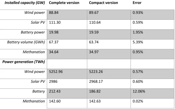
Table 1 presents the installed capacities for each of the non-dispatchable technologies and battery storage, and the power production from each of these technologies over the 19 years.

Table 1. Installed capacity for endogenous technologies in the complete version of EOLES_elecRES model and in its compact version with the corresponding error values. Both models are optimised over a 19-weather-year period (2000-2018).

Installed capacity (GW) Complete version Compact version Error

Wind power 88.84 89.67 0.93% Solar PV 111.30 110.64 0.59% Battery power 19.98 19.59 1.95% Battery volume (GWh) 67.37 63.74 5.39% Methanation 34.64 34.97 0.95% Power generation (TWh) Wind power 5252.96 5223.26 0.57% Solar PV 2986 2968.17 0.60% Battery 212.43 186.82 12.06% Methanation 142.60 142.63 0.02%

As shown, the error is below 2% for wind power, solar PV, battery power and methanation. Higher errors occur for battery volume and generation.

(13)

12

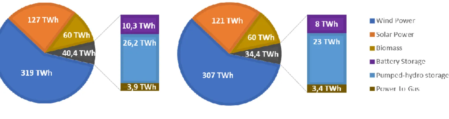
Figures 2 and 3 show the power production and installed capacity by technology.

Figure 2. Installed capacity of each technology in GW for the complete and compact versions of the EOLES_elecRES model

Table 2 summarizes the cost and load curtailment observed from the complete model and its compact version. Errors are below 1% for system cost and load curtailment. The compact version underestimates the storage loss by 3% (but by only 0.16 percentage points), presumably due to the lower use of battery storage.

Figure 3. Power production for the complete and compact versions of the EOLES_elecRES model

The variable time-step method reduces the number of time-steps from 166,440 to 28,027, i.e. a six-fold decrease in the time-related indices. This six-fold decrease leads to a reduction in calculation time from nearly one week to around one hour for the 19-year optimization. Applying this method to the

(14)

single-13

year simulation with 8,760 time-steps, model execution time is reduced from 10 minutes to 10 seconds, i.e. a 60-fold gain in time.

Table 2. Annualized cost, COST, load curtailment and storage related losses for the complete and compact versions of the EOLES_elecRES model

Output Complete version Compact version Error

Annualized cost (b€/year) 20.90 20.77 0.62%

Average system cost (€/MWh) 49.49 49.18 0.62%

Load curtailment % 11.27 11.26 0.09%=0.01 perc. pts

Storage loss % 5.17 5.01 3.09%=0.16 perc. pts

On the basis of these indicators, we can conclude that the variable time-step method provides a huge gain in optimization time, with very low discrepancies in aggregate variables (cost, load curtailment, storage loss). In the next section we check whether this conclusion stands when we change the cost of two storage options: batteries and methanation. We vary the cost of storage, not generation

technologies, because the key challenge for our method is to correctly reproduce storage technology capacity and operation in spite of the coarser temporal resolution. We do not change the cost of pumped hydro because its capacity is limited by assumption.

b. Results for the EOLES_elecRES model, sensitivity analysis

In this subsection, we present the comparison between the complete and compact versions of the EOLES_elecRES model optimized over 19 weather-years for four alternative cost scenarios: battery 25% more expensive, battery 25% cheaper, methanation 25% more expensive and methanation 25% cheaper3. The results can be found in Tables A.4 to A.7 in Appendix 5.

3

PEM electrolysers for different dimensions are forecasted to cost between €350/kW and €550/kW in 2050 (ENEA, 2017). The value we chose to represent was 450€/kW, and the boundaries of the projection vary by 22.5%. According to same reference, methanation isothermal reactor is expected to fall from €1000/kW to €700/kW (a 30% cost reduction), and the catalytic methanation process is not a mature process with high uncertainties. Therefore, all together representing methanation, we defined an uncertainty range of ±25%.

(15)

14

To better understand the absolute error over each important variable, we present the boxplots of these errors for the five scenarios in Figure 4. These show that the variable time-step method performs very well with respect to installed capacity and power production by technology, as well as to the

methanation (long-term) storage option, and the overall system cost. While the installed power capacity of battery storage is estimated with great precision, its volume is underestimated by about 5% and its power generation by around 11%.

Load curtailment and storage loss are generally estimated with an error of less than 2%, but for the case of the cheap power-to-gas scenario the error reaches 5% in both cases. Overall, the main conclusions relating to the reliability of the variable time-step method are robust to uncertainty about storage technology cost.

Figure 4. Absolute error boxplots for the five cost scenarios

c. Results for the DIETER model

As detailed in subsection 2.b and appendix 4, we ran the DIETER model with renewable technologies alone as generation options and three main storage technologies with no DSM options for the year 2013

Battery storage energy volume capex is estimated at USD150/kWh (€125/kWh at the current market exchange rate) by Cole and Frazier (2019) in 2050, while BNEF (2017) projects a more optimistic cost: €75/kWh (both for 2035 and 2050). Our central cost scenario (Schmidt et al, 2019) projects €100/kWh for battery storage in the stationary utility-level use. Therefore, we considered 25% variation in the cost of batteries as well. -2.00% 0.00% 2.00% 4.00% 6.00% 8.00% 10.00% 12.00% 14.00% 16.00%

(16)

15

for the German power system data (Zerrahn et al, 2015). The complete version of this model has an overall simulation time of 1310 seconds, of which 202 seconds for the CPLEX solution, while the remainder is for LP generation and data loading. The compact version has an overall simulation time of 25 seconds, with 10 seconds of CPLEX time and 12 seconds of LP generation and data loading.

Therefore, this method leads to a 52-fold reduction in the solution time for a one-year simulation, a result close to that obtained with the EOLES_elecRES model.

Figures 5 and 6 show power production and installed capacity by technology for both the complete and compact versions of DIETER. We present the installed capacity and power production errors in Appendix 6. As for EOLES_elecRES, the errors in the installed generation capacities are below 2%, while they are higher (up to 17%) for storage technologies, especially batteries. The annualized cost for the complete version is €48.05bn/year while the annualized cost for the compact version is €48.66bn/year, an over-estimation of only 1.25%.

(17)

16

Figure 6. Power production for the complete and compact versions of DIETER

These results confirm the initial findings of the variable time-step method as applied to the

EOLES_elecRES model, i.e. we observe a huge gain in computation time with very small errors in the most important variables: system cost and power generation mix.

4. Discussion and conclusion

We have developed a new method (the ‘variable time-step method’) to reduce the optimization time of energy system models and applied it to the dispatch and investment optimization models

EOLES_elecRES (Shirizadeh et al., 2020) and DIETER (Zerrahn and Schill, 2015). The variable time-step method allows calculation time to be reduced by a factor of 50 to 60.

The price to pay in terms of accuracy is small: for both models and for contrasted cost scenarios, the error in system cost is around 1%. For the generation capacity in wind, solar PV and biomass, the error remains below 2%. For curtailment and storage loss, it remains below half a percentage point. The only sizable error concerns battery volume and generation, but it remains below 20% in the worst case (the DIETER model for battery power capacity). Our method underestimates the required electricity generation from, and capacity of, batteries. Battery storage technology can be fully charged and discharged in less than 4 hours (energy volume to power capacity ratio), while in this method, daily-subsampling leads to time-slices of 5 hours and even more. This may explain the relatively low precision in battery modelling. As we defined a reserve constraint for the hydro-reserve correction, similar correction constraints for battery storage could be defined but to do so, a deeper analysis of the battery charge and discharge dynamics is required. Further work is required to fully understand and correct this discrepancy.

(18)

17

Our method brings greater accuracy and much faster optimization than if we use a constant temporal resolution coarser than one hour. For instance, running EOLES_elecRES with time-steps of 6 hours speeds up the calculation by a factor of only 36 (compared with ca. 60 for our method) but

underestimates the system cost by 3%, overestimates the solar PV capacity by 17% and underestimates the battery volume by 18%. Our method should be useful for any large-scale model featuring long-term storage, including other technologies than those considered here, such as power-to-heat with storage (Bloess et al., 2018). For models applied at a subnational local level, the definition of critical periods would be more difficult because ideally it should be based not only on the residual load, but also on imports and exports of electricity. In any case, we consider that this method might contribute to the improvement in computational tractability that is required to cope with the increasing complexity of energy system models, thus making further research into the method worthwhile.

References

ADEME (2015). Vers un mix électrique 100 % renouvelable.

https://www.ademe.fr/sites/default/files/assets/documents/mix-electrique-rapport-2015.pdf

Arditi, M., Durdilly, R., Lavergne, R., Trigano, É., Colombier, M., Criqui, P. (2013). Rapport du groupe de travail 2: Quelle trajectoire pour atteindre le mix énergétique en 2025 ? Quels types de scénarios possibles à horizons 2030 et 2050, dans le respect des engagements climatiques de la France ? Tech. rep., Rapport du groupe de travail du conseil national sur la Transition Energétique

Blanford, Geoffrey J., James H. Merrick, John E. T. Bistline, and David T. Young. Simulating Annual Variation in Load, Wind, and Solar by Representative Hour Selection. Energy Journal, 2018: 189-212

Bloess, A., Schill, W. P., & Zerrahn, A. (2018). Power-to-heat for renewable energy integration: A review of technologies, modeling approaches, and flexibility potentials. Applied Energy, 212, 1611-1626.

Böhme, D. (Ed.). (2012). Erneuerbare energien in zahlen: Nationale und internationale entwicklung. BMU.

(19)

18

Bramstoft, R., Pizarro-Alonso, A., Jensen, I. G., Ravn, H., & Münster, M. (2020). Modelling of renewable gas and renewable liquid fuels in future integrated energy systems. Applied Energy, 268, 114869.

Brown, T. W., Bischof-Niemz, T., Blok, K., Breyer, C., Lund, H., & Mathiesen, B. V. (2018). Response to ‘Burden of proof: A comprehensive review of the feasibility of 100% renewable-electricity systems’. Renewable and sustainable energy reviews, 92, 834-847

Cole, W., and A. W. Frazier. (2019). Cost Projections for Utility-Scale Battery Storage. Golden, CO: National Renewable Energy Laboratory. NREL/TP-6A20-73222.

https://www.nrel.gov/docs/fy19osti/73222.pdf.

Collins, S., Deane, P., Gallachóir, B. Ó., Pfenninger, S., & Staffell, I. (2018). Impacts of inter-annual wind and solar variations on the European power system. Joule 2(10), 2076-2090

Ding, X., Liu, L., Huang, G., Xu, Y., & Guo, J. (2019). A Multi-Objective Optimization Model for a Non-Traditional Energy System in Beijing under Climate Change Conditions. Energies, 12(9), 1692.

ENEA Consulting (2016). The potential of Power-to-Gas.

https://www.enea-consulting.com/sdm_downloads/the-potential-of-power-to-gas/

ENTSO-E. Consumption Data. European Network of Transmission System Operators for Electricity, 2014. URL https://www.entsoe.eu/db-query/consumption/mhlv-a-specific-country-for-a-specific-month.

FCH JU (2015). Commercialisation of energy storage in Europe: Final report. Fuel Cells and hydrogen joint undertaking. https://www.fch.europa.eu/publications/commercialisation-energy-storage-europe

Green, R., I. Staffell and N. Vasilakos (2014). Divide and Conquer? k-Means Clustering of Demand Data Allows Rapid and Accurate Simulations of the British Electricity System. IEEE Transactions on Engineering Management, 2014: 251-260.

Hoffmann, M., Kotzur, L., Stolten, D., & Robinius, M. (2020). A Review on Time Series Aggregation Methods for Energy System Models. Energies, 13(3), 641.

Hourdin, F., Foujols, M. A., Codron, F., Guemas, V., Dufresne, J. L., Bony, S., ... & Braconnot, P. (2013). Impact of the LMDZ atmospheric grid configuration on the climate and sensitivity of the IPSL-CM5A coupled model. Climate Dynamics, 40(9-10), 2167-2192.

(20)

19

JRC (2014) Energy Technology Reference Indicator Projections for 2010–2050. EC Joint Research Centre Institute for Energy and Transport, Petten.

JRC (2017) Cost development of low carbon energy technologies - Scenario-based cost trajectories to 2050, EUR 29034 EN, Publications Office of the European Union, Luxembourg, 2018, ISBN 978-92-79-77479-9, doi:10.2760/490059, JRC109894.

Mavrotas, G.; Diakoulaki, D.; Florios, K.; Georgiou, P. (2008). A mathematical programming framework for energy planning in services’ sector buildings under uncertainty in load demand: The case of a hospital in Athens. Energy Policy, 36, 2415–2429.

Moraes, L., Bussar, C., Stoecker, P., Jacqué, K., Chang, M., & Sauer, D. U. (2018). “Comparison of long-term wind and photovoltaic power capacity factor datasets with open-license.” Applied Energy 225, 209-220.

Murray, P., Orehounig, K., & Carmeliet, J. (2020). Multi-objective optimisation of power-to-mobility in decentralised multi-energy systems. Energy, 117792.

Nahmmacher, Paul, Eva Schmid, Lion Hirth, and Brigitte Knopf (2016). Carpe diem: A novel approach to select representative days for long-term power system modeling. Energy, 2016: 430-442

Nitsch, J., Pregger, T., Naegler, T., Heide, D., de Tena, D. L., Trieb, F., ... & Trost, T. (2012). Langfristszenarien und Strategien für den Ausbau der erneuerbaren Energien in Deutschland bei Berücksichtigung der Entwicklung in Europa und global. Schlussbericht im Auftrag des BMU, bearbeitet von DLR (Stuttgart), Fraunhofer IWES (Kassel) und IfNE (Teltow), 345.

Palmintier, B. (2014). Flexibility in generation planning: Identifying key operating constraints. In 2014 power systems computation conference (pp. 1-7). IEEE, August.

Pape, C., Gerhardt, N., Härtel, P., Scholz, A., Schwinn, R., Drees, T., ... & Sailer, F. (2014). Roadmap Speicher-Bestimmung des Speicherbedarfs in Deutschland im europäischen Kontext und Ableitung von technisch-ökonomischen sowie rechtlichen Handlungsempfehlungen für die Speicherförderung. Fraunhofer IWES, Kassel.

Pfenninger, S., Staffell, I. (2016). “Long-term patterns of European PV output using 30 years of validated hourly reanalysis and satellite data.” Energy 114, pp. 1251-1265. doi: 10.1016/j.energy.2016.08.060

(21)

20

Pfenninger, S. (2017). Dealing with multiple decades of hourly wind and PV time series in energy models: A comparison of methods to reduce time resolution and the planning implications of inter-annual variability. Applied energy, 197, 1-13.

Pineda, S.; Morales, J.M. (2018). Chronological Time-Period Clustering for Optimal Capacity Expansion Planning With Storage. IEEE Trans. Power Syst., 33, 7162–7170.

Regelleistung (2014). Daten zur Regelenergie, https://www.regelleistung.net/ip/action/abrufwert.

RTE (2018), Panorama de l’électricité renouvelable au 30 Juin 2018.

Samsatli, S.; Samsatli, N.J. (2015). A general spatio-temporal model of energy systems with a detailed account of transport and storage. Comput. Chem. Eng., 80, 155–176.

Schill, W. P., & Zerrahn, A. (2018). Long-run power storage requirements for high shares of renewables: Results and sensitivities. Renewable and Sustainable Energy Reviews, 83, 156-171.

Schmidt, O., Melchior, S., Hawkes, A., Staffell, I. (2019). Projecting the Future Levelized Cost of Electricity Storage Technologies. Joule ISSN 2542-4351 https://doi.org/10.1016/j.joule.2018.12.008

Schröder, A., Kunz, F., Meiss, J., Mendelevitch, R., & Von Hirschhausen, C. (2013). Current and prospective costs of electricity generation until 2050 (No. 68). DIW data documentation.

Seljom, P., Rosenberg, E., Fidje, A., Haugen, J. E., Meir, M., Rekstad, J., & Jarlset, T. (2011). Modelling the effects of climate change on the energy system—A case study of Norway. Energy policy, 39(11), 7310-7321.

Shirizadeh, B., Perrier, Q., & Quirion, P. (2019). How sensitive are optimal fully renewable power systems to technology cost uncertainty?. FAERE PP 2019-04,

http://faere.fr/pub/PolicyPapers/Shirizadeh_Perrier_Quirion_FAERE_PP2019.04.pdf

Shirizadeh, B., Perrier, Q., & Quirion, P. (2020). EOLES_elecRES model description. CIRED working papers, n° 2020-80, February 2020.

(22)

21

Staffell, I., Pfenninger, S. (2016). “Using Bias-Corrected Reanalysis to Simulate Current and Future Wind Power Output.” Energy 114, pp. 1224-1239. doi: 10.1016/j.energy.2016.08.068

Victoria, M., Zhu, K., Brown, T., Andresen, G. B., & Greiner, M. (2019). The role of storage technologies throughout the decarbonisation of the sector-coupled European energy system. Energy Conversion and Management, 201, 111977.

Zerrahn, A., & Schill, W. P. (2015). A greenfield model to evaluate long-run power storage requirements for high shares of renewables. DIW Discussion Papers No. 14057

Zeyringer, M., Price, J., Fais, B., Li, P. H., & Sharp, E. (2018). Designing low-carbon power systems for Great Britain in 2050 that are robust to the spatiotemporal and inter-annual variability of weather. Nature Energy 3 (5), 395

(23)

22

Appendix 1. Definition of critical periods and daily sub-sampling for EOLES_elecRES model

To set the duration of the critical periods (those which require an hourly resolution) we chose several periods to cover various difficult situations that must be overcome by the power system. The hours with the highest residual demand are of great importance since the installed capacity should be sufficient to satisfy peak residual demand. Batteries can be fully discharged in less than four hours; we therefore chose the four-hour period with the highest residual load as a second critical period duration. The longest period should be chosen in such a way that short-term and mid-term storage options (batteries and PHS) are modelled correctly. We achieved this by identifying the periods during which the state of charge of these two storage options declines from the maximum to zero and tracing them using histograms (Figure A.1).

Figure A.1. Histograms of discharge time for PHS and battery storage

As shown, the PHS discharge time rarely exceeds four days, therefore we chose the 96-hour period with the highest residual demand as the longest critical period, within which every hour is represented as a single time-step. Since adding a limited number of time-steps does not significantly change the solution time, we added six-hour, twelve-hour, one-day and two-day periods in between the previously

mentioned critical periods.

The next step is to group the remaining hours in a coherent way. We have prepared a daily power production and consumption profile by taking an average over each day of the 18-year period for which results have been previously calculated (Shirizadeh et al. 2019). Figure A.2 shows this typical day including all technologies (left) and including only dispatchable technologies (right).

(24)

23

Figure A.2. Average typical day for the 18-year period simulation, with (left) and without (right) non-dispatchable technologies

Using the power production profiles and focusing on the dispatchable technologies, we can divide the typical day into four time-steps:

1. Morning, from 7 am to 10 am, a transition period during which non-dispatchable generation rises steeply.

2. Noon, 10 am to 3 pm, the period with the maximum excess non-dispatchable generation, which determines required storage volume.

3. Evening, 3 pm to 10 pm, the period with the highest residual demand, resulting in massive use of dispatchable technologies.

4. Night, 10 pm to 7 am, a period during which residual demand is low, resulting in little use being made of dispatchable technologies, but storage technologies can be charged during this period.

Appendix 2. JRC 2017 cost projection methodology and scenarios

In this JRC report, historic installed capacity of each technology for 2015, learning rate related to each technology and the capital investment cost of each technology in 2015 have been taken as input values, and using three different future installed capacity scenarios, three different future cost trajectories are proposed. Equation (A1) shows the main methodology used in the cost projection using the learning rate method:

𝐶𝑜𝑠𝑡_𝑡 = 𝐶𝑜𝑠𝑡₀∙ (𝐶𝑡 𝐶0)

𝛿

(A.1)

This log-linear relation relates the future cost (𝐶𝑜𝑠𝑡𝑡) of a technology to the existing cost (𝐶𝑜𝑠𝑡0), existing installed capacity (𝐶0) and the future projected installed capacity (𝐶𝑡) of it using the experience

(25)

24

parameter 𝛿. The learning rate LR is related to the experience parameter as it is described in equation (A.2);

𝐿𝑅 = 1 − 2𝛿 _(A.2)

The JRC report uses three different scenarios to project the future installed capacity of each technology, and finally to find the _𝐶𝐶𝑡

0 ratio for the equation (16). These three scenarios are described in Table A.1;

Table A.1 the chosen scenarios by JRC for the 2050 cost projections of low carbon power production technologies Scenario

Baseline This scenario is used to cover the lower end of RES-E deployment. It is based on the "6DS" scenario of the Energy Technology Perspectives published by the International Energy Agency in 2016. It represents a "business as usual" world in which no additional efforts are taken on stabilizing the atmospheric concentration of greenhouse gases. By 2050, primary energy consumption reaches about 940 EJ, renewable energy supplies about 30 % of global electricity demand and emissions climb to 55 GtCO2.

Diversified The "Diversified" portfolio scenario is taken from the "B2DS" scenario of the International Energy Agency's 2017 Energy Technology Perspectives and is used as representative for the mid-range deployment of RES-E found in literature. To achieve rapid decarbonization in line with international policy goals, all known supply, efficiency and mitigation options are available and pushed to their practical limits. Fossil fuels and nuclear energy participate in the technology mix, and CCS is a key option to realize emission reduction goals. Primary energy consumption is comparable to 2015 levels (about 580 EJ), the share of renewable electricity in the global supply mix is 74 % while emissions decline to about 4.7 GtCO2 by 2050.

ProRES The "ProRES" scenario results are the most ambitious in terms of capacity additions of RES-E technologies. In this scenario the world moves towards decarbonization by significantly reducing fossil fuel use, however, in parallel with rapid phase out of nuclear power. CCS does not become commercial and is not an available mitigation option. Deep emission reduction is achieved with high deployment of RES, electrification of transport and heat, and high efficiency gains. It is based on the 2015 "Energy Revolution" scenario

(26)

25

of Greenpeace. Primary energy consumption is about 430 EJ, renewables supply 93 % of electricity demand and global CO2 emissions are about 4.5 GtCO2 in 2050.

The used economical parameters for the power production technologies are taken from the 2050 projections of this study for the diversified scenario as an average and more realistic scenario.

Appendix 3. Input data for EOLES_elecRES model

A.3.a. VRE profiles

Variable renewable energies’ (offshore and onshore wind and solar PV) hourly capacity factors have been prepared using the renewables.ninja website4, which provides the hourly capacity factor profiles of solar and wind power from 2000 to 2018 at the geographical scale of French counties (départements), following the methods elaborated by Pfenninger and Staffell (2016) and Staffell and Pfenninger (2016). These renewables.ninja factors reconstructed from weather data provide a good approximation of observed data: Moraes et al. (2018) finds a correlation of 0.98 for wind and 0.97 for solar power with the observed annual duration curves (in which the capacity factors are ranked in descending order of magnitude) provided by the French transmission system operator (RTE).

To prepare hourly capacity factor profiles for offshore wind power, we first identified all the existing offshore projects around France using the “4C offshore” website5, and using their locations, we extracted the hourly capacity factor profiles of both floating and grounded offshore wind farms. The Siemens SWT 4.0 130 has been chosen as the offshore wind turbine technology because of recent increase in the market share of this model and its high performance. The hub height of this turbine is set to 120 meters.

A.3.b. Electricity demand profile

Hourly electricity demand is ADEME (2015)’s central demand scenario for 2050. This demand profile falls in the middle of the four proposed demand scenarios for 2050 in France by Arditi et al. (2013) during the national debates on the French energy transition (DNTE).

4_{https://www.renewables.ninja/}

5

(27)

26

A.3.c. Cost data

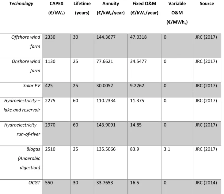
The economic parameters for generation technologies are taken from JRC (2014, 2017). We added the grid upgrading cost of €24.6/kW for new renewable power plants to the capital expenditure values of each VRE technology which is mandated by the transport system operator RTE and by the distribution system operator ENEDIS (RTE, 2018). Table A.2 summarizes the economic parameters for different technologies and theirs sources.

Table A.2 Economic parameters of power production technologies Technology CAPEX (€/kWe) Lifetime (years) Annuity (€/kWe/year) Fixed O&M (€/kWe/year) Variable O&M (€/MWhe) Source Offshore wind farm 2330 30 144.3677 47.0318 0 JRC (2017) Onshore wind farm 1130 25 77.6621 34.5477 0 JRC (2017) Solar PV 425 25 30.0052 9.2262 0 JRC (2017) Hydroelectricity – lake and reservoir

2275 60 110.2334 11.375 0 JRC (2017) Hydroelectricity – run-of-river 2970 60 143.9091 14.85 0 JRC (2017) Biogas (Anaerobic digestion) 2510 25 135.5066 83.9 3.1 JRC (2017) OCGT 550 30 33.7653 16.5 0 JRC (2014)

(28)

27

The Economic parameters of storage technologies are gathered from various sources. Table A.3 summarizes these parameters and their sources;

Table A.3 Economic parameters of storage technologies Technology Overnight costs (€/kWe) CAPEX (€/kWhe) Lifetime (years) Annuity (€/kWe/year) Fixed O&M (€/kWe/year) Variable O&M (€/MWhe) Storage annuity (€/kWhe/year) Efficiency (input / output) Source Pumped hydro storage (PHS) 500 5 55 25.8050 7.5 0 0.2469 95%/90% FCH-JU (2015) Battery storage (Li-Ion) 140 100 12.5 15.2225 1.96 0 10.6340 90%/95% Schmidt (2019) Methanation 1150 0 20/25* 87.9481 59.25 5.44 0 59%/45% ENEA (2016)

Appendix 4. Application of ‘variable time-step’ method to DIETER model

To apply the variable time-step method to DIETER, we first set the installed capacities of all non-renewable generation technologies to zero. Therefore, the only electricity production technologies studied are offshore and onshore wind power, solar power, run-of-river and biomass. Similarly, to keep the same storage technologies as in the EOLES_elecRES model, we fixed the installed power and energy capacities of NaS, lead acid and redox flow batteries and CAES to zero. Li-ion batteries, pumped-hydro storage and power-to-gas are the only storage technologies considered, as per Zerrahn and Schill’s (2015) baseline scenario. Demand-side management options are all set to zero, so that the main flexibility providers are storage options and biomass. To allow curtailment of excess renewable power generation, we modified the supply-demand balance equation (equation 4 in Zerrahn and Schill, 2015), from equality to inequality, and removed the DSM components, hence this equation becomes:

𝑑_ℎ+ ∑ 𝑆_{𝑠𝑡𝑜,ℎ}𝑖𝑛

𝑠𝑡𝑜 ≤ ∑𝑐𝑜𝑛(𝐺𝑐𝑜𝑛,ℎ𝑙 + 𝛽𝑐𝑜𝑛,ℎ) + ∑𝑟𝑒𝑠𝐺𝑟𝑒𝑠,ℎ+ ∑𝑠𝑡𝑜𝑆𝑠𝑡𝑜,ℎ𝑜𝑢𝑡 (A.3)

Where 𝑑ℎ is hourly inelastic demand, 𝑆𝑠𝑡𝑜,ℎ𝑖𝑛 is the charging of storage technology 𝑠𝑡𝑜 at hour ℎ, 𝐺𝑐𝑜𝑛,ℎ𝑙 is the hourly generation level of conventional technology 𝑐𝑜𝑛, 𝛽𝑐𝑜𝑛,ℎ is the reserve provision from the

(29)

28

conventional technology 𝑐𝑜𝑛 at hour ℎ, 𝐺𝑟𝑒𝑠,ℎ is the hourly generation from renewable technology 𝑟𝑒𝑠 and 𝑆𝑠𝑡𝑜,ℎ𝑜𝑢𝑡 is the discharging of storage technology 𝑠𝑡𝑜 at hour ℎ.

In addition to the above changes, the compact version of the DIETER model includes corrections of time-step length in the equations relating the installed capacity to power production and reserve provisions. Similarly, we added the hydro-reservoir correction (equation 9) to the maximum inflow and outflow equations for pumped-hydro storage technology. The codes and input data for the compact version can be found on GitHub6.

We apply the variable time-step method as discussed previously. We define the critical periods as those with the highest residual demands and introduce hourly time-steps for their whole duration. The average daily power production and storage profile for the year 2013 is presented in Figure 2. For non-critical periods, we applied the same daily downsampling as with EOLES_elecRES. Critical period definition and daily downsampling resulted in 1,626 time-steps.

Figure A.3 Average day for 2013 with the DIETER model for Germany

Appendix 5. Sensitivity of the variable time-step method to cost scenarios

Tables A.4 to A.7 summarize the results of the sensitivity analysis that has been applied to the 19 year-long version of EOLES_elecRES model and the compact version developed using variable time-step method. The varying parameters are battery storage cost (+/-25%) and methanation cost (+/-25%).

6 https://github.com/BehrangShirizadeh/dieter_compact/ -20000 0 20000 40000 60000 80000 -20000 0 20000 40000 60000 80000 0 1 2 3 4 5 6 7 8 9 10 11 12 13 14 15 16 17 18 19 20 21 22 23 G en era tio n (MW)

hour of the day

Average day

offshore onshore PV biomass river battery

(30)

29

Table A.4 Results for the expensive battery scenario

Wind power 101.23 100.89 0.34%

Solar PV 104.24 104.83 0.57%

Battery power 17.63 17.32 1.76%

Battery volume (GWh) 48.47 46.27 4.54%

Methanation 35.95 36.34 1.08%

Power generation (TWh) Complete version Compact version Error

Wind power 5547.21 5465.32 1.48%

Solar PV 2796.70 2812.52 0.57%

Battery 153.23 137.09 10.53%

Methanation 144.17 148.64 0.78%

Output Complete version Compact version Error

Average system cost (€/MWh)

50.27 49.87 0.80%

(31)

30

Table A.5 Results for the cheap battery scenario

Wind power 82.57 82.84 0.33%

Solar PV 123.25 121.51 1.41%

Battery power 23.19 22.82 1.60%

Methanation 32.35 32.65 0.93%

Wind power 4856.76 4836.15 0.42%

Solar PV 3306.65 3259.88 1.41%

Battery 355.99 326.04 8.41%

Methanation 134.91 135.61 0.52%

48.32 48.00 0.66%

(32)

31

Table A.6 Results for the cheap power-to-gas scenario

Wind power 90.21 90.53 0.35%

Solar PV 107.88 108.25 0.34%

Battery power 18.80 18.59 1.12%

Methanation 35.65 35.87 0.62%

Wind power 5145.71 5109.58 0.70%

Solar PV 2894.28 2904.17 0.34%

Battery 210.08 184.79 12.04%

Methanation 207.64 201.18 3.11%

48.23 47.91 0.66%

(33)

32

Table A.7 Results for the expensive power-to-gas scenario

Wind power 92.43 92.31 0.13% Solar PV 112.70 111.34 1.21% Battery power 20.45 20.04 2% Battery volume (GWh) 74.03 68.94 6.88% Methanation 33.97 34.10 0.38% Power generation (TWh) Wind power 5436.17 5398.98 0.68% Solar PV 3023.43 2987.16 1.20% Battery 188.18 161.60 14.12% Methanation 88.62 93.34 5.33% Output

50.26 49.91 0.70%

(34)

33

Appendix 6. Results for DIETER model

Table A.8 Results of the complete and compact versions for DIETER model, and the precision of the compact model

Complete model Compact model Ratio (x)

overall time (s) 1310 25 52,4

load time (s) 1090,14 12 90,845

CPLEX time (s) 202 10,22 19,7651663

Complete model Compact model Error (%)

cost (b€/an) 48,05 48,66 1,25% battery_power (GW) 10,89 9,02 17,17% battery_volume (GWh) 34,66 35,98 3,67% PHS_power (GW) 25,43 26,61 4,43% PHS_volume (GWh) 300 300 0,00% P2G_power (GW) 3,65 3,72 1,88% P2G_volume (GWh) 154,06 140,37 8,89% Offshore_power (GW) 32 32 0,00% Offshore_energy (TWh/an) 126,254 125,26 0,79% Onshore_power (GW) 137,05 139,75 1,93% onshore_energy (TWh/an) 192,914 181,37 5,98% Wind_power_aggregated 169,05 171,75 1,57% Wind_energy_aggregated 319,168 306,63 3,93% PV_power (GW) 155,93 157,33 0,89% PV_energy (TWh/an) 126,706 120,5 4,90% Biomass_power (GW) 38,65 39,36 1,80% Biomass_energy (TWh/an) 60 60 0,00%