A strategy for climate evaluation of aircraft technology: an efficient climate impact assessment tool ? AirClim

(1)

HAL Id: hal-00303061

https://hal.archives-ouvertes.fr/hal-00303061

Submitted on 17 Aug 2007

HAL is a multi-disciplinary open access

archive for the deposit and dissemination of sci-entific research documents, whether they are pub-lished or not. The documents may come from teaching and research institutions in France or abroad, or from public or private research centers.

L’archive ouverte pluridisciplinaire HAL, est destinée au dépôt et à la diffusion de documents scientifiques de niveau recherche, publiés ou non, émanant des établissements d’enseignement et de recherche français ou étrangers, des laboratoires publics ou privés.

A strategy for climate evaluation of aircraft technology:

an eﬀicient climate impact assessment tool ? AirClim

V. Grewe, A. Stenke

To cite this version:

V. Grewe, A. Stenke. A strategy for climate evaluation of aircraft technology: an eﬀicient climate impact assessment tool ? AirClim. Atmospheric Chemistry and Physics Discussions, European Geo-sciences Union, 2007, 7 (4), pp.12185-12229. �hal-00303061�

(2)

ACPD

7, 12185–12229, 2007

Climate impact assessment tool:

AirClim

V. Grewe and A. Stenke

Title Page Abstract Introduction Conclusions References Tables Figures ◭ ◮ ◭ ◮ Back Close

Full Screen / Esc

Printer-friendly Version Interactive Discussion

EGU

Atmos. Chem. Phys. Discuss., 7, 12185–12229, 2007 www.atmos-chem-phys-discuss.net/7/12185/2007/ © Author(s) 2007. This work is licensed

under a Creative Commons License.

Atmospheric Chemistry and Physics Discussions

A strategy for climate evaluation of

aircraft technology: an efficient climate

impact assessment tool – AirClim

V. Grewe and A. Stenke

Deutsches Zentrum f ür Luft- und Raumfahrt, Institut f ür Physik der Atmosph äre, Oberpfaffenhofen, 82230 Wessling, Germany

Received: 9 August 2007 – Accepted: 13 August 2007 – Published: 17 August 2007 Correspondence to: V. Grewe (volker.grewe@dlr.de)

(3)

ACPD

7, 12185–12229, 2007

AirClim

Full Screen / Esc

EGU Abstract

Climate change is a challenge to society and to cope with requires assessment tools which are suitable to evaluate new technology options with respect to their impact on climate. Here we present AirClim, a model which comprises a linearisation of the pro-cesses occurring from the emission to an estimate in near surface temperature change,

5

which is presumed to be a reasonable indicator for climate change. The model is de-signed to be applicable to aircraft technology, i.e. the climate agents CO₂, H₂O, CH₄ and O3(latter two resulting from NOx-emissions) and contrails are taken into account. It employs a number of precalculated atmospheric data and combines them with aircraft emission data to obtain the temporal evolution of atmospheric concentration changes,

10

radiative forcing and temperature changes. The linearisation is based on precalculated data derived from 25 steady-state simulations of the state-of-the-art climate-chemistry model E39/C, which include sustained normalised emissions at various atmospheric regions. The results show that strongest climate impacts from ozone changes occur for emissions in the tropical upper troposphere (60 mW/m2; 80 mK for 1 TgN emitted),

15

whereas from methane in the middle tropical troposphere (–2.7% change in methane lifetime; –30 mK per TgN). The estimate of the temperature changes caused by the individual climate agents takes into account a perturbation lifetime, related to the re-gion of emission. A comparison of this approach with results from the TRADEOFF and SCENIC projects shows reasonable agreement with respect to concentration changes,

20

radiative forcing, and temperature changes. The total impact of a supersonic fleet on radiative forcing (mainly water vapour) is reproduced within 5%. For subsonic air traf-fic (sustained emissions after 2050) results show that although ozone-radiative forcing is much less important than that from CO2 for the year 2100. However the impact on temperature is of comparable size even when taking into account temperature

de-25

creases from CH₄. That implies that all future measures for climate stabilisation should concentrate on both CO2and NOxemissions. A direct comparison of super- with sub-sonic aircraft (250 passengers, 5400 nm) reveals a 5 times higher climate impact of

(4)

ACPD

7, 12185–12229, 2007

AirClim

Full Screen / Esc

EGU

supersonics.

1 Introduction

Air traffic has the potential to grow over-proportional compared to other transport sec-tors. Its specific climate impact, i.e. relative to fuel consumption is larger than for other sectors (Fuglestvedt et al., 20071). One reason is the higher altitude of the emission,

5

which leads to longer atmospheric residence times, particularly in the case of NOx emissions and its chemical products (ozone, methane).

Therefore, there is a need to develop technical and operational options to reduce the impact from air traffic emissions on climate and to provide tools to reliably assess these impacts, or at least to provide some metrics for various technology options within

10

a range of uncertainty.

In this context it is important to note that a simple metric based on fuel consumption or emission indices insufficiently describes the total climate impact. The dependency of the strength of the impact on altitude and region cannot be described by such met-rics. For example, contrail formation depends on aircraft design aspects (propulsion

15

efficiency), water vapour emission (directly related to fuel consumption), but also and equally important on local atmospheric conditions (Schumann et al.,2000).

We concentrate on near surface temperature changes as a metric for climate change, as we think it is the most suitable metric for our purpose. Other metrics, e.g. global warming potentials, have been widely discussed (Fuglestvedt et al.,2003;Shine et al.,

20

2005) and a time-integrated radiative forcing including its efficacy has been chosen to be appropriate. Sausen and Schumann (2000) presented a linear response model, which allows estimates of near surface temperature changes based on precalculated radiative forcings, which are combined with a transient emission scenario to take into

1

Fuglestvedt, J., Berntsen, T., Myhre, G., Rypdal, K., and Skeie, R.: Climate forcing from the Transport Sectors, PNAS, submitted, 2007.

(5)

ACPD

7, 12185–12229, 2007

AirClim

Full Screen / Esc

EGU

account accumulation effects, e.g. for CO2. This means that the climate response of a given radiative forcing is linearised in this approach to calculate the associated temperature change. Response functions were derived on the basis of an ocean-atmosphere model.

Here we present an assessment tool, which is an extension to the linear response

5

model described in Sausen and Schumann (2000). The extension comprises a lin-earisation of the relation between emissions of CO₂, NO_x and H₂O and impacts on atmospheric composition related to carbon dioxide, ozone, methane, water vapour, and contrails. Note that in our approach spatially resolved emissions are taken into ac-count in contrast toSausen and Schumann(2000) who concentrated on annual global

10

values. Hence, the input to the AirClim model are 3-D aircraft emission data, precal-culated atmospheric data and some parameters describing the overall evolution of air traffic and some background concentrations, which are all converted into a timeseries of near surface temperature changes.

A detailed description of the methodology is given in Sect.2, followed by a

descrip-15

tion of the atmospheric input data, i.e. a description of the simulation results employing idealised emission scenarios. These are forming the basis for the linearisation of chem-ical and radiative responses. A validation of the chemchem-ical and radiative responses is given in Sect. 4 by comparing them to detailed climate-chemistry simulations. In Sec-tion 5 some applicaSec-tions are presented with respect to sub- and supersonic air traffic.

20

2 Methodology

2.1 Overview

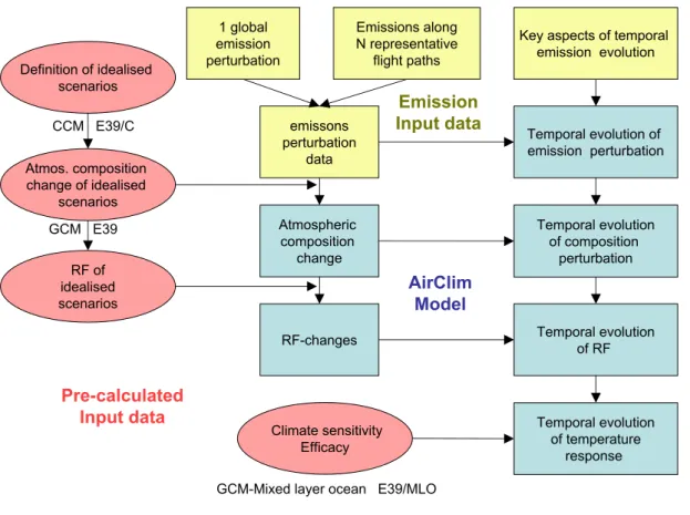
An overview of the methodology is given in Fig.1. The main part of the model AirClim is indicated in blue, showing the functional chain from emissions (yellow) and precalcu-lated atmospheric input data (rose) to the resulting global mean near surface

temper-25

(6)

ACPD

7, 12185–12229, 2007

AirClim

Full Screen / Esc

EGU

precalculated atmospheric input data is given in the next section. These data describe the Jacobian of the atmosphere-chemistry system with respect to emissions of CO₂, NOx, and H2O, or in other words the atmospheric sensitivity to regional emissions. 2.2 Precalculated input data

In the first step we define emission regions with a normalised (=equal for all regions)

5

emission strength (in mass mixing ratios per time). Then, in a second and third step chemical perturbations and radiative forcing of CO2, ozone, methane, water vapour, and contrails are calculated applying a state-of-the-art climate-chemistry model (here: E39/C). These results will then be linearly combined with emission perturbation data to obtain perturbation patterns of chemical species and the associated radiative forcing

10

(Sect.2.4).

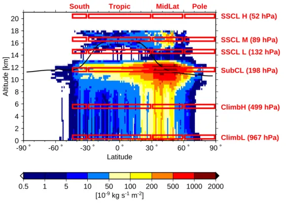
2.2.1 Idealised emission regions

Emission regions are presented in Fig.2(see also Tables1and2). We have defined areas for three potential supersonic cruise levels (SSCL). Since the impact will depend on the geographical distribution, also 4 latitudinal bands are taken into account.

Addi-15

tionally, three levels for subsonic air traffic are included to represent take-off, climb and cruise. This leads to 24 regions.

Since we mainly concentrate on supersonic (stratospheric) air traffic, we limited the number of flight levels to a subsonic fleet. However, the methodology is set-up in a way that additional emission regions can easily be added, refining the methodology.

20

For each of the regions a uniform emission is defined, which is derived from the SCENIC dataset: At 50◦_{N the zonally integrated fuel consumption varies between 500} and 2000×10−9_kg/s/m2

and 200 and 500×10−9_kg/s/m2

for subsonic (≈12 km) and su-personic cruise levels (18–19 km), respectively. This relates to 62–247×10−15_kg/kg/s and 77–192×10−15_{kg/kg/s, respectively. Mean values are chosen to represent these}

25

(7)

ACPD

7, 12185–12229, 2007

AirClim

Full Screen / Esc

EGU

2.2.2 Chemical composition

For each of the idealised emission regions, a climate-chemistry simulation is performed employing a normalised emission of nitrogen oxides and water vapour to obtain the chemical response of an emission in that region. We applied the climate-chemistry model E39/C (Hein et al., 2001), in which we accounted for full Lagrangian

trans-5

port (ATTILA, Reithmeier and Sausen, 2002) of all species including water vapour and cloud water, which significantly improved the representation of stratospheric water vapour and temperatures (Stenke et al., 20072). E39/C consists of the troposphere-stratosphere climate model ECHAM4.L39(DLR) (E39, Land et al., 1999) and the troposphere-stratosphere chemistry module CHEM (Steil et al., 1998). Recently, a

10

number of revisions were released (Dameris et al.,2005). An overview of validation activities is given inGrewe(2006).

The experimental set-up comprises a steady-state simulation (time-slice) for the year 2050, which means boundary conditions, like background CO2, CH4, N2O, and CFC concentrations, emissions of NOxfrom industry, biomass burning, transport, and soils

15

and sea surface temperatures represent predicted conditions for the year 2050. They are prescribed according toIPCC(2001) or are taken from coupled ocean-atmosphere model simulations. Latter applies for ocean temperatures. Background aircraft emis-sions include subsonic aircraft (SCENIC-database, scenario S4, Marizy et al. (2007)3, see also Table4). This defines a base case simulation. Twenty-four perturbation

sim-20

ulations, one for each emission region, are performed including an additional constant emission of NO_xand H₂O (see above). After a spin-up time, five consecutive years are calculated in order to obtain annual mean changes.

Figure 3 shows exemplarily for the two emission regions SSCL-H/Pole (top) and

2

Stenke, A., Grewe, V., and Ponater, M.: Lagrangian transport of water vapor and cloud water in the ECHAM4 GCM and its impact on the cold bias, J. Climate, revised, 2007b.

3

Marizy, C., Rogers, H., and Pyle, J.: The SCENIC emission database, Atmos. Chem. Physc. Dissc., in preparation, 2007.

(8)

ACPD

7, 12185–12229, 2007

AirClim

Full Screen / Esc

EGU

SSCL-M/Pole (bottom) changes in water vapour (left), nitrogen oxides (NO_y, mid), and ozone (right). Water vapour (left) shows an increase of around 150 ppbv and 100 ppbv at high northern latitudes for high and mid supersonic cruise levels, which corresponds to an increase of around 9 and 6%, respectively. In the stratosphere the loss processes are similar for water vapour and nitrogen oxides (NOy) perturbations, therefore the

life-5

times and hence the change pattern of the perturbations are almost identical in the stratosphere. The impact on ozone (Fig.3, right) strongly depends on altitude and lat-itude of the perturbation. The climate-chemistry model E39/C shows a transition from ozone increase to ozone decrease roughly 4 km above the tropopause for the case of the mid supersonic cruise level (bottom). Ozone decrease is the stronger the higher

10

the emissions occurs (top). The decrease in stratospheric ozone is compensated by a tropospheric increase as seen in the simulation for the mid supersonic cruise level (bottom).

2.2.3 Contrail coverage

Contrail coverage is calculated by folding the potential contrail coverage (Fig.6) with

15

flight data. The potential contrail coverage is the maximum possible coverage in the case that aircraft are flying everywhere at any time. It is calculated with E39/C including a parametrisation for line-shaped contrails (Ponater et al.,2002). According toSausen

et al. (1998) a linear scaling including a non-physical parameter (see also below) folded with the flown distance provides the actual coverage. Contrails may occur in regions,

20

which are both cold and humid enough so that additional water vapour leads to cloud formation (Fig.6). These regions are limited to the tropopause area (see thick line for the location of the tropopause).

2.2.4 Radiative forcing of idealised perturbation scenarios

To each of the perturbation scenarios the stratospheric adjusted radiative forcing is

25

(9)

ACPD

7, 12185–12229, 2007

AirClim

Full Screen / Esc

EGU

are performed with a length of 15 months which include the annual mean perturbation patterns derived from the chemical composition change simulations (2.2.2), following the methodology byStuber et al.(2001). The annual mean is calculated based on the last 12 months.

2.2.5 Climate sensitivity and efficacies

5

Although changes in chemical species may lead to the same radiative forcing their impact on climate (temperature) may differ significantly (Stuber et al.,2001;Joshi et al.,

2003). This relationship is expressed in terms of climate sensitivity, i.e. the change in near surface temperature relative to a normalised radiative forcing (1 W/m2) or in terms of efficacies (Hansen et al.,2005), which are these climate sensitivity parameters

10

normalised to that of CO2. Efficacies for a variety of climate agents are taken from literature (Ponater et al.,2005,2006). Those values are derived from long-term steady-state simulations applying a coupled ocean-atmosphere model (here: E39 coupled to a mixed layer ocean model) to a well defined radiative forcing. The ratio of the temperature perturbation to the radiative forcing gives the climate sensitivity for that

15

kind of perturbation. The values used are identical to those in Grewe et al. (2007) (their Table 7).

2.3 Emission data

The aim of the application of the model AirClim is to compare technological options for aircraft with respect to a climate change metric and a UV-change metric. The latter is

20

only important for supersonic transport and can be omitted for subsonic applications. Hence, at least three emission dataset are needed: A base case scenario and two scenarios which include perturbations or technological options to the base case and which are aimed to be intercompared. In principle two approaches are applicable. If enough knowledge is available on the future development of the considered fleet,

25

(10)

ACPD

7, 12185–12229, 2007

AirClim

Full Screen / Esc

EGU

used, i.e. this refers to the case of normal passenger aircraft, where present traffic is well known and estimates for future traffic exist (e.g. Marizy et al., 20073). However, in the case of business jets, even nowadays traffic is only poorly known and future developments are even less explored. In this case, we suggest to take an arbitrary base case (e.g. Marizy et al., 20073). For a perturbation scenario emissions are added to

5

the base case. For these perturbations city pairs for flight connections can be chosen, whose flight paths are somehow equally distributed over the globe. These city pairs are used for all technology options considered. A linear combination (to differently weight each region) of the emissions along the flight paths is used as an estimate for the considered fleet emissions. The weighting of the regions, i.e. the linear combination

10

is somehow arbitrary and therefore object to an uncertainty analysis (see below). In all cases at least 3 three-dimensional emission datasets are considered and serve as input to the model AirClim.

In addition, a general temporal development of the base case air traffic has to be considered to take into account accumulation effects, e.g. of CO2 emissions. Further,

15

a year has to be defined, when the technology options are taken in service and a year (Tconst) for which the 3-D emission data discussed above are representative (here: Tconst=2050). For the present investigation, we suggest to keep the emissions constant for all scenarios after this date. One reason is that the composition change simulations (see Sect.2.2.2) are 5 year steady-state simulations and hence are based on constant

20

emissions. Further this date is far in the future (2050) so that projections are highly uncertain, anyway. However, other scenarios may well be taken into account. In any case, the impact is somehow limited, since all scenarios are compared to the base case in the end. Figure7shows an example of emission scenarios, which are used in the validation Section (Sect.4).

25

2.4 Linear response model: AirClim

The model AirClim (see Fig. 1) combines the precalculated (Sect. 2.2) altitude and latitude dependent perturbations with the emission data (Sect.2.3) to obtain a metric

(11)

ACPD

7, 12185–12229, 2007

AirClim

Full Screen / Esc

EGU

for climate change.

2.4.1 Transient emissions, concentration and radiative forcing changes

The development of the base case CO2emission and concentration changes are de-fined by input parameters. CO₂emissions of the perturbation scenarios are calculated by integrating the emissions along the flight paths, which are representative for the year

5

Tconst. They are exponentially interpolated between the time of in-service and Tconst. The resulting changes in the concentration of CO₂ are calculated using a constant lifetime of 100 years.

The concentration changes of all other species are calculated for a time Tconst+τspecies withτspecies the lifetime of the respective species. It takes into account

10

that the precalculated concentration patterns are derived from steady-state simula-tions. In detail, the concentration changes of a speciesCspecies(e.g., ozone and water vapour) for a perturbation scenario are calculated by folding the emissions along the flight paths with the precalculated scenarios:

Cspecies= 1 T ZT 0 Especies(t) X X k ǫ_k(t) C_{i d}species(i_k, j_k) M(ik, jk) d t , (1) 15

where ǫk(t) (k = 1, ..., 4) are weights for the four surrounding emissions regions

(i_k, j_k) (i_k=latitude, jk=pressure level) at a certain point of the flight path, C

species

id (ik, jk)

the concentration change in [kg/kg] from the idealised scenario (ik, jk) (Tables 1 and 2), M(ik, jk) the respective mass of air in the idealised emission region in [kg], and

Especies(t) the emission of species in [kg/s]. Note that Cspecies and C_idspecies(i_k, j_k)

20

are 2-dimensional fields. X is the respective normalised emission strength (Table3). X ×M(ik, jk) then gives the emission rate (in kg/s) in the idealised emission region.

Other quantities are derived in a similar way, e.g. the radiative forcing is derived by replacing C_idspecies in Eq. (1) by the radiative forcingRF_idspecies (Fig. 4c,d). Changes in methane lifetime, the lifetimes of tropospheric ozone and stratospheric quantities are

(12)

ACPD

7, 12185–12229, 2007

AirClim

Full Screen / Esc

EGU

derived accordingly, considering either tropospheric or stratospheric emissions only. The 100 hPa level is used for the separation between troposphere and stratosphere. A climatological tropopause based on temperature profiles would be feasible, however emissions in the lowermost stratosphere have also a limited lifetime, which is more similar to the upper troposphere than mid stratosphere.

5

The change in methane is then derived by regarding the difference of two linear differential equations for background methane (CCH4_{) and the perturbation (}_CCH4 ₊

∆CCH4_{), which both have the same production terms and the loss differs by the change}

in methane lifetime, resulting in d d t∆C CH₄ = δ 1 + δτ −1 CH₄C CH₄ − 1 1 + δτ −1 CH₄∆C CH₄_, (2) 10

whereδ is the relative change in lifetime, τ

CH4 the methane lifetime (here: 9 years) and

CCH4_{the background methane concentration, e.g. taken from}_IPCC₍₂₀₀₁_{). A temporal}

evolution of the change of the methane lifetime is achieved by scaling it with normalised CO2emission, such thatδ(T

const

+ τ_CH4)=δ.

The temporal evolution of concentration changes Cspecies(t) of tropospheric ozone 15

and stratospheric quantities (ozone and water vapour) is calculated by solving a simple linear differential equation taking the respective lifetime into account. Since we regard only changes relative toCspeciesatTconst+τspecies, we scale the concentration changes so that they are 1 at that time, i.e. Cspecies(Tconst+ τspecies)=1. A proportionality is assumed between changes in methane and its radiative forcing (IPCC,1999).

20

In principle changes in contrail coverage can be estimated applying the identical methodology as for ozone and water vapour, by applying Eq. (1). However, contrail occurrence is more constrained to altitudes around the tropopause (see Fig.6), which requires a higher vertical resolution of the idealised scenarios than currently performed. Therefore, we suggest here an alternative method. The potential contrail coverage

pre-25

sented in Fig.6is used and linearly folded with data of flown distance, which leads to a 2-D contrail coverage (see also Sect. 4 and Fig. 8c, e). The advantage is that the

(13)

ACPD

7, 12185–12229, 2007

AirClim

Full Screen / Esc

EGU

horizontal and vertical resolution is much better resolved with 48*39=1872 gridpoints compared to 24 if only the idealised scenarios are applied. Global total contrail cover-age is calculated by vertical summation taking into account maximum random overlap (Manabe and Strickler,1964). The non-physical scaling parameterγ=0.00166 s m2/km is chosen such that the global value is identical to a reference 3-D GCM simulation (see

5

below) applying the SCENIC database. Contrail radiative forcing is calculated by apply-ing a linear relationship between contrail coverage and radiative forcapply-ing: 6.384 W/m2 for 100% total contrail coverage (Stenke et al., 20074).

2.4.2 Temperature change

The temperature change caused by the perturbation scenarios is calculated following

10

the approach ofSausen and Schumann(2000):

∆T = ZT t₀ G(t − t ′₎ _RF∗₍_t′₎ _{d t}′_, ₍₃₎ with G(t − t′_{) = αe}−t−t′τ , with ₍₄₎ α = 2.246/36.8K

a and τ = 36.8a and

15 RF∗₍_{t) =} X species RFspecies RFCO₂ λ eff species ∆Ci(t) R R Cspecies_{d p dl at} (5)

∆T describes the perturbation temperature with respect to the base case, G the Green’s function for the near surface temperature response and RF∗ _{the normalised} radiative forcing. Because of the small changes in the concentration, especially for

4

Stenke, A., Grewe, V., and Pechtl, S.: Do supersonic aircraft avoid contrails?, At-mos. Chem. Physc. Discuss., 7, in preparation, 2007a.

(14)

ACPD

7, 12185–12229, 2007

AirClim

Full Screen / Esc

EGU

CO2, saturation effects are omitted, different to the approach by Sausen and Schu-mann (2000).

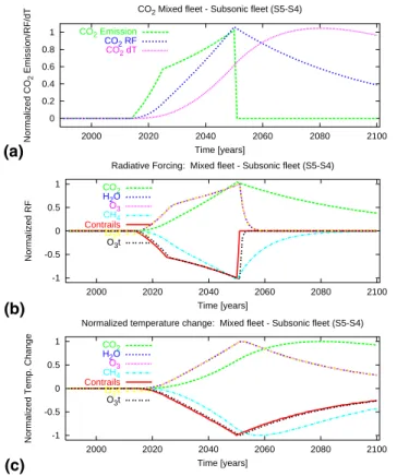
In order to illustrate the relationship between emission, radiative forcing and tem-perature change, as well as the impact of different lifetimes of atmospheric tracers, a thought experiment is given in Fig. 7. We consider an increase in emissions up

5

to the year 2050 and switch them off afterwards (Fig. 7a). A supersonic impact sce-nario is taken as emission scesce-nario, i.e. the SCENIC mixed fleet minus subsonic fleet scenario (Grewe et al.,2007) (S5–S4), where the first HSCT aircraft are in service in 2015, a second generation evolves in 2025 and the full fleet is established in 2050. Again for illustrative reasons, all time series are normalised to their maximum values.

10

Figure7a illustrates the relation between CO₂emissions, radiative forcing and temper-ature changes. The radiative forcing from CO2slowly decreases after 2050, mirroring the relatively long lifetime of CO2. Temperature increase peaks much later (around 2080) caused by the inertia of the ocean-atmosphere system.

Other species show different behaviour for radiative forcing (Fig.7b) (and their

con-15

centration, not shown) and the associated temperature increase (Fig.7c) according to the lifetime of the regarded species: Contrails and tropospheric ozone have shorter lifetimes, hence radiative forcing decreases more rapidly than that of stratospheric wa-ter vapour, methane and CO2. Maximum temperature change is found for contrails and tropospheric ozone changes around 2050, whereas methane peaks around 2060 and

20

CO2around 2080.

3 Atmospheric sensitivity to emissions

In order to evaluate the chemical impact of air traffic emissions 25 simulations (1 base case and 24 perturbations, see Fig.2) with the climate-chemistry model E39/C are per-formed (see above) for each of the selected emission region. These precalculated data

25

(with respect to the application of AirClim) describe the sensitivity of the atmosphere to the emission region. Since the emission regions do not have the same air mass, the

(15)

ACPD

7, 12185–12229, 2007

AirClim

Full Screen / Esc

EGU

results presented in Fig.3are not directly intercomparable. In contrast, the lifetimes of the perturbations, i.e. the mass of the perturbation divided by the emission strength are directly intercomparable. Figure4a shows the lifetimes of the perturbations for every emission region. For the polar region the water vapour perturbation has a lifetime of 13 months, whereas at lower altitudes the lifetime decreases to 9 and 4.3 months for

5

the mid and low supersonic cruise altitude. At subsonic cruise levels the lifetime of a water vapour perturbation amounts to around 1 month and is less than 1 h for climb and take-off.

Changes in ozone and water vapour also have an impact on the concentration of the hydroxyl radical (OH). The reaction of OH with methane (CH4) is the dominant

10

tropospheric methane loss process. Although methane changes are calculated in the idealised scenarios, they do not represent the steady-state methane change, basi-cally for two reasons. First, methane has a lifetime of around 8 to 9 years, which implies that a far longer simulation time is necessary to accurately calculate methane changes. Second, at the surface, methane is prescribed to correctly represent

tro-15

pospheric methane. This offsets methane changes to some extend. For that reason methane loss rates from the reaction with the hydroxyl-radical (OH) are calculated and converted into a methane lifetime. Changes in this methane lifetime are deduced from the difference in the background and perturbation simulation. Additionally, a factor of 1.4 is taken into account for reductions in the loss rates due to the boundary condition

20

(IPCC,1999). Figure4b shows relative changes (%) in tropospheric methane lifetime for the 24 emission regions. Two regions can be identified, where an emission of NOx reduces methane lifetime most: The stratosphere at high supersonic cruise level, as already indicated in the results of the ozone change (see above) and the tropical tropo-sphere (–2.7% change in methane lifetime at 500 hPa and –2.5% at 200 hPa for 1 TgN

25

emitted), where chemistry is fast and reacts more sensitively to emissions. Minimum changes are found at tropopause levels, where chemistry is generally slow and OH formation limited by either water vapour concentration and UV irradiance.

(16)

ACPD

7, 12185–12229, 2007

AirClim

Full Screen / Esc

EGU

emission of 1 Pg H2O and 1 TgN, respectively. The effects from water vapour emis-sions qualitatively follow the pattern of the respective lifetime (Fig.4a) and leads to a warming independent of the location of the emissions. In the extra-tropics no sensi-tivity to the respective latitude of the emission is found, in contrast to ozone (Fig.4d). NOx emissions show largest impact on ozone radiative forcing in the tropical upper

5

troposphere with a large latitudinal gradient from 60 mW/m2 per 1 TgN emitted to less than 5 mW/m2at higher latitudes. In contrast, NOxemissions at high supersonic cruise altitude lead to a negative radiative forcing at mid and high latitudes and hence to a decrease of near surface temperature.

In order to intercompare the climate impact of a unit emission in the emission regions,

10

i.e. the regional dependency of the near surface temperature change to the emission region, we have applied AirClim for the pre-defined emission regions (Fig.2; Table3) with a normalised emission strength. The strength of the emission is secondary, since we focus on the regional patterns. However, the ratio of water vapour emissions, i.e. fuel consumption, to NOx emissions is important. Here we take the mean value

15

from the SCENIC subsonic emission data (S4; EI(NOx)=10.85 g(NO2)/kg(fuel)). Fig-ure5 shows the near surface temperature change for 2100 as a function of altitude and latitude of the emission (note that we assume steady-state for the period 2050 to 2100). The temperature increase due to water vapour changes and the tempera-ture decrease due to methane changes (Fig.5a, c) reflect directly their lifetime pattern

20

(Fig.4a). The temperature changes due to water vapour and ozone (5a, b) also reflect their radiative forcing (Fig.4c, d). Although the lifetime of methane changes is consid-erably larger than for ozone it does not compensate for the smaller radiative forcing. Hence ozone changes from NOxemissions dominate the temperature change over the compensating methane effect (Fig.5d), at least for this specific emission index of NOx,

25

or smaller indices. Figure 5e shows the sum of all effects. Clearly, the higher the al-titude of an emission the larger is its climate impact. There is also a clear difference between tropical and extra-tropical emission locations, with a lower climate impact at high latitudes.

(17)

ACPD

7, 12185–12229, 2007

AirClim

Full Screen / Esc

EGU 4 Validation of the linearisation approach

The basic question is, whether linearisation of the effect of emissions on the chemical composition and contrail coverage is applicable to aircraft emissions. This is investi-gated by comparing results from a detailed climate-chemistry simulation (E39/C) with the results of the linearised model AirClim. In the detailed simulation, E39/C is applied

5

to calculate ozone, water vapour and contrail cover changes and the associated radia-tive forcing. In the linearised approach the precalculated perturbations of the chemical composition and contrail cover as well as their respective radiative forcing are folded with the emission data set. Hence, two simulations for each model are performed, one including emissions of water vapour and nitrogen oxides from a subsonic fleet and

an-10

other one, which includes emissions from a mixed sub- and supersonic fleet, where 500 subsonic aircraft are replaced by supersonics in a way that the passenger trans-port volume is unaffected. A more detailed discussion of the chemical impacts is given inGrewe et al.(2007) and a discussion of the contrail impacts in Stenke et al. (2007)4. Here we concentrate on the differences between the detailed and the linearised

ap-15

proach.

Figure8shows the results for E39/C (top) and AirClim (bottom) for the difference of the two model simulations, i.e. the impact of a partial replacement of subsonic aircraft by supersonics. Clearly, magnitude and pattern of the change in water vapour is similar in both models. Maximum values of around 300 ppbv are found in both models on the

20

northern hemisphere at around 70 hPa, decreasing to around 30 ppbv at tropopause altitudes. However, differences occur on tropical and southern latitudes, where the water vapour enhancement is underestimated by 50% in AirClim. Clearly, the low res-olution in AirClim, where the whole atmosphere is resolved by 24 gridpoints compared to 180 000 gridpoints in E39/C, leads to numerical diffusion. Note, that only radiative

25

forcing values will further be taken into account for calculating temperature changes, which are not calculated based on the fields presented in Fig.8, but calculated from the radiative forcing of the idealised scenarios.

(18)

ACPD

7, 12185–12229, 2007

AirClim

Full Screen / Esc

EGU

Both models show a similar pattern in ozone changes (Fig.8middle column) caused by a partial substitution of subsonic air traffic. Ozone depletion peaks in the tropical stratosphere at around 10 hPa and at northern mid-latitudes at around 50 hPa. In the troposphere a distinct difference is found between northern and southern hemisphere with a decrease and increase in ozone, respectively. Absolute values of ozone changes

5

differ only slightly between the models.

Contrail formation changes for both models are shown in Figs.8c, f. The results for the linearised model are scaled with the non-physical parameterγ to give the same global contrail coverage (see Sect. 2.4.1) for this reference case. Note that for all other applications to emission datasets this parameter remains unchanged. The global

10

pattern is very similar in both simulations. A decrease in contrail coverage due to the replacement of subsonic aircraft is compensated by a tropical increase in contrail coverage. Both simulations show a good agreement of the pattern, e.g. an increase in contrail coverage at some subsonic cruise levels, i.e. where supersonic aircraft fly at subsonic speed (over land).

15

Table5shows the radiative forcing from the substitution of parts of a subsonic fleet by supersonics (SCENIC S5-S4 scenario) as calculated byGrewe et al. (2007) (top) and with the AirClim model. Clearly, water vapour, the dominant climate agent in this case, is well reproduced. Other parameters, which are an order of magnitude smaller show larger deviations. In general, the more complex the chemical and physical

pro-20

cesses are the larger are the deviations. Water vapour is mainly dynamically controlled, whereas ozone and methane are dynamically and chemically controlled. The linearisa-tion of methane effects includes the longest funclinearisa-tional chain among all of the species regarded.

Hence the linearisation of transport, chemistry, contrail formation and radiation is

25

working sufficiently well. The pattern and absolute values of concentration changes are well reproduced and the total radiative forcing agrees within 3.6% between the linearised model AirClim and the non-linear climate-chemistry model E39/C.

(19)

ACPD

7, 12185–12229, 2007

AirClim

Full Screen / Esc

EGU 5 Climate impact of air traffic

In this section a first application of AirClim is performed with respect to subsonic and supersonic air traffic. We are focusing on the importance of CO2versus NO_xemissions for subsonic air traffic, a climate impact minimization for options of supersonics and the difference between sub- and supersonic transport with respect to climate change. The

5

numerical efficiency of the linearised model facilitates the analysis of a number of air traffic scenarios, which would not be possible applying climate-chemistry models.

Although AirClim has been designed, as a first step, to be applicable to supersonic transport, it basically can be applied to all kind of 3-D emission data. However, the coarse vertical resolution in the area of subsonic transport limits its applicability, which

10

is described in more detail below. In future, we will enhance this resolution in order to achieve a full applicability with respect to air traffic.

In our study, we concentrate on the TRADEOFF aircraft emission data (Sausen et al.,

2005) for the year 2000 and the SCENIC emission data (Marizy et al., 20073) for the years 2025 and 2050 (Table4) since for those datasets also radiative forcing estimates

15

are available. For the period prior to 2000 we take historical records into account (IPCC,1999).

5.1 Subsonic air traffic: TRADEOFF and SCENIC

Table 6 shows the comparison of radiative forcing from Sausen et al. (2005), which are based on a number of model simulations, with AirClim, for the year 2000. The

20

results obtained with AirClim are similar to those in Sausen et al. (2005) and within the range of uncertainty given therein. Differences in CO2 may occur due to an as-sumption of exponential temporal interpolation between given historical values for fuel consumption, which slightly decreases the accumulation of CO2. Larger differences occur for methane, where AirClim shows a lower sensitivity compared to the mean

25

value in Sausen et al. Again, the values are still in the range of uncertainty.

(20)

ACPD

7, 12185–12229, 2007

AirClim

Full Screen / Esc

EGU

subsonic flight altitude, whereas for water vapour the sensitivity is very large. Hence in the present state AirClim is not able to correctly represent the water vapour radiative forcing from subsonic air traffic. The vertical resolution of AirClim is not sufficient to resolve the water vapour impact at tropopause regions. To obtain reasonable values for water vapour radiative forcing from subsonic air traffic we have multiplied this value

5

by 0.25 to overcome this deficiency for the further discussion of the temperature effects. The water vapour impact is regarded to be small for subsonic air traffic, anyway (IPCC,

1999;Sausen et al.,2005).

Figure9a presents the temporal evolution of temperature changes derived with Air-Clim for the above described emission scenario. Note that again the emissions are

10

kept constant after the year 2050 for illustration purpose. For short-term perturba-tions (ozone, contrails and water vapour) the temperature change reaches equilibrium in less than 100 years after the emissions are kept constant. Species with a longer atmospheric lifetime (CH₄and CO₂) reach steady-state after around 150 years.

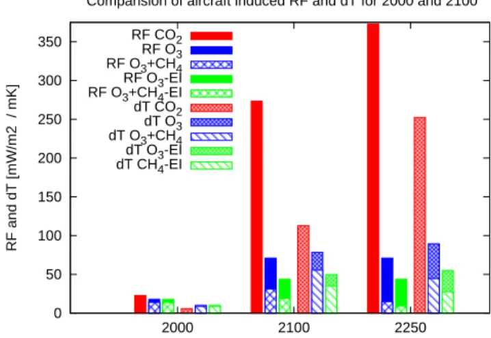
In Fig. 10 we compare the climate impact of CO2 and NOx emissions of subsonic

15

air traffic for the year 2000, 2100, and 2250 applying the metrics radiative forcing and temperature change. Note that the year 2250 is only taken into account to represent steady-state. There is no other meaningful interpretation, since the results largely depend on the assumptions of the air traffic scenario.

For all points of time radiative forcing from CO₂is larger than the radiative forcing of

20

the products of NOxemissions, i.e. ozone and the sum of ozone and methane (left three bars at each date). However, the temperature changes (right three bars at each date), ozone and methane are larger than for CO₂in the year 2000. This is a consequence of the larger efficacy of ozone (=1.4) compared to CO2(=1) (see Sect.2.2.5). In 2100 the difference between the temperature change caused by CO2and ozone (as well as

25

ozone plus methane) is less than 50%, although the radiative forcing of CO₂is 3 and 5 times larger than for ozone and the sum of ozone plus methane, respectively. Only at steady-state (year 2250) the climate impact of CO2 emissions clearly dominates over NO_xemissions.

(21)

ACPD

7, 12185–12229, 2007

AirClim

Full Screen / Esc

EGU

Therefore, although CO₂emissions have a much larger atmospheric residence time, its climate impact in terms of near surface temperature changes is of comparable size to that of NOxemissions via ozone formation and methane loss. A reduction of the NOx emission index by 40% between 2000 and 2050, which will result in an emission index of 6 g(NO2) per kg fuel as e.g. discussed as an option for future technology (Ponater

5

et al., 2006) is shown by green boxes. This reduction will lower the importance of NO_xemissions. Still the temperature change induced by the NO_xemissions will not be negligible.

5.2 Supersonic air traffic and mitigation options: SCENIC

Figure9b shows the temporal evolution of near surface temperature changes for a

re-10

placement of 500 subsonic aircraft by supersonics. A detailed discussion of the impact of such a replacement is given in Grewe et al. (2007). They applied 4 atmosphere-chemistry models (including E39/C) to investigate the climate impact and the impact on ultraviolet radiation for different options of a supersonic fleet.

Figure 9b shows the same main features as Fig. 9a in Grewe et al. (2007).

Wa-15

ter vapour is the main contributor to climate change with regard to a supersonic fleet. Differences occur with respect to ozone since the mean value among 4 applied atmosphere-chemistry models was negative inGrewe et al. (2007), whereas here we calculate a small positive value. The turn around point between ozone increase at lower levels and ozone depletion at higher altitudes for a specific NOx emission is

20

still a major uncertainty (Grewe et al., 2007). Wuebbles et al. (2004) investigated the impact of the emission altitude on ozone column with a two-dimensional model and found a turnaround point between 13 km and 15 km, whereas E39/C simulates it around 14.5 km and 16.5 km. Currently, we are not able to include this uncertainty in AirClim. However, for the future one could include it, if multiple input data, precalculated

25

by different models were used (see Sect.2.2).

In the study byGrewe et al.(2007), E39/C was one of the applied models. However it was only applied to one of the options for computational reasons. Since AirClim is

(22)

ACPD

7, 12185–12229, 2007

AirClim

Full Screen / Esc

EGU

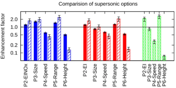
numerically efficient, it can be applied to all of the scenarios, i.e. a higher NOxemission index (P2), a doubling of the fleet size (P3), a decreased speed from Mach 2 to Mach 1.6 (P4), an increased range (P5), and a decreased cruise altitude (P6). Figure 11

is the analogous figure to their Figure 10 showing the impact of these options as a relative change with respect to the base case mixed fleet scenario (S5). The metrics

5

near surface temperature change (blue filled bars) and ozone depletion (blue dashed bars) are taken into account. Since the options do not account for the same super-sonic transport volume, we additionally normalised the results to the same supersuper-sonic transport volume (red bars). The product of the two metrics is than given as an overall metric (green bars).

10

In principle, the results lead to the same conclusions as in Grewe et al. (2007), i.e. the scenarios P6 (cruise altitude) and P4 (speed) show the smallest environmental impact. Differences occur especially in the calculated temperature change caused by an increased emission index of NO_x(P2) and increased range (P5). Note, that the er-rorbars express different ranges of uncertainty in Fig. 10 inGrewe et al.(2007) and our

15

Fig.11. Grewe et al. (2007) include, whenever possible, uncertainties covered by the range of model results, whereas in AirClim this uncertainty cannot be estimated, since only E39/C has been applied to derive the precalculated input data (Sect.2.2). Differ-ences are still within the range of uncertainty indicated by these errorbars, except for P5 and P6. The temperature increase derived for scenario P5 and the ozone depletion

20

in scenario P6 significantly differs between the two approaches. The main difference between the findings for P5 and P6 and all other scenarios is that those results are only obtained by one model (SLIMCAT). Therefore, the results are somehow biased towards this model. An uncertainty range for ozone depletion could not be provided in

Grewe et al.(2007) for the same reasons. Anyway, the main conclusion indicated by

25

their results is the same.

The SCENIC scenarios discussed above are not suitable for a direct intercompari-son of a subintercompari-sonic and superintercompari-sonic aircraft, since the impact of the replaced subintercompari-sonic cannot be evaluated. Therefore an additional scenario (S4core) has been calculated

(23)

ACPD

7, 12185–12229, 2007

AirClim

Full Screen / Esc

EGU

which includes only those subsonic aircraft, which are not replaced by supersonics in the mixed fleet scenario (Egelhofer, personal communication). Hence the difference between S4 and S4core and the difference between S5 and S4core refers to aircraft with the same characteristics and transport volume.

Figure12shows the direct intercomparison between those subsonic and supersonic

5

aircraft, i.e. the impact of scenario S4 minus S4core (crossed) and the impact of sce-nario S5 minus S4core (filled). The results clearly show that the total climate impact of supersonics is approximately 5 times of that from subsonic aircraft. The fuel consump-tion for the subsonics, which are replaced is around 20 Tg/year compared to 60 Tg/year for the supersonics. This well explains the radiative forcing and temperature changes

10

with respect to CO2. The large difference in near surface temperature change arises predominantly from large water vapour changes, which are a consequence of the high emission altitude and the longer atmospheric residence times.

6 Conclusions

In this study we have proposed a methodology to assess the climate impact of

emis-15

sions from air traffic. The main climate agents with respect to super- and subsonic air traffic are CO2, H₂O, O₃, CH₄, and contrails. The functional chain from emissions to climate change of these species is complex and includes transport, chemistry, mi-crophysics, and radiation. We have shown that the linearisation of these processes is possible and can be used within a more simple climate assessment tool, which

facil-20

itates the numerical efficient conversion of emission datasets into a metric of climate change. Here we propose near surface temperature changes in 2100 as a metric.

In order to linearise a complex climate-chemistry model (here: E39/C) we performed simulations applying a number of idealised emission scenarios. The results of these scenarios give insights into the atmospheric response, in terms of radiative forcing

25

and temperature change to normalised emissions. Water vapour emissions show an increasing climate impact the higher or the closer to the tropics the emissions

(24)

oc-ACPD

7, 12185–12229, 2007

AirClim

Full Screen / Esc

EGU

cur. Ozone from NO_xemissions has the largest warming potential at tropical latitudes around 100 to 200 hPa. Methane reduction caused by NOxemissions is included. Al-though methane tends to reduce the warming and alAl-though atmospheric residence times are larger than those for ozone the overall effect of NOx emissions is still one of a warming. The NOx effect is reversed at high supersonic cruise levels, where NOx

5

leads to ozone depletion.

Stevenson et al.(2004) suggested that the integrated ozone radiative forcing could be outweighted by the methane impact when regarding short-term pulse emissions. In our study we find a significant reduction by approximately 50% of the near surface temperature response. The differences are to some extend arising from the larger

10

ozone climate sensitivity, which is not taken into account in Stevenson et al. (2004), since they concentrated on radiative forcing, whereas we were focusing on near surface temperature changes.

Similar approaches to calculate the temperature changes caused by air traffic emis-sions have been used previously (Sausen and Schumann,2000;Ponater et al.,2006;

15

Ling et al.,2006;Lukachko et al.,2006;Grewe et al.,2007). They are all based on the same relationship between radiative forcing and temperature. Here we revised those methods with two main characteristics. First, the calculation of the radiative forcing for a specific emission dataset is included in the AirClim model by linearising these pro-cesses instead of precalculating them with detailed climate-chemistry models. Hence

20

the place of the emission as well as its strength plays a key role in the determination of the radiative forcing. Second, we introduced typical residence times for stratospheric and tropospheric perturbations and for methane. With this, each regarded species has a typical residence time, which is perturbed by the air traffic emissions. Hence, the tem-poral development of ozone and methane perturbations differ remarkably in contrast to

25

earlier studies.

The results performed for a subsonic fleet (TRADEOFF, SCENIC) show good agree-ment with previously calculated values for radiative forcing (Sausen et al.,2005). The calculated temperature change clearly shows that in future, e.g. 2100, CO₂ becomes

(25)

ACPD

7, 12185–12229, 2007

AirClim

Full Screen / Esc

EGU

the most important contributor to air traffic induced climate change, however NOx emis-sions closely follow even when taking counteracting methane responses into account and also some challenging reductions in the emission index of NOx. The regarded sce-nario assumes a constant fleet after 2050, which is probably unrealistic, but reasonable to illustrate the response to a steady-state. Assuming a further increase would even

5

increase the importance of ozone compared to CO2, because the short-term effects from the increase in ozone due to an increase in air traffic and emissions dominate over long-term effects resulting from increasing CO2 concentrations due to its long lifetime. This applies as long as air traffic increases considerably. That implies that all future measures for climate stabilisation should concentrate on both CO₂ and NO_x

10

emissions.

Because of an extension to the SCENIC database we were able to directly compare subsonic and supersonic aircraft, in the sense that transport volume is the same and aircraft themselves are comparable. Such a comparison has not been performed so far (IPCC,1999;Grewe et al.,2007). Instead, the impacts of a whole mixed fleet have

15

been compared to a whole subsonic fleet. Our results show that supersonic aircraft of this size (250 passenger, 5400 nm range) have a five times larger climate impact than their subsonic counterpart. Smaller supersonic jets, e.g. business jets (e.g. 8 passenger 3500 nm) are also likely to have a larger climate impact than their subsonic counterparts. However, the enhancement is probably less than for larger aircraft, since

20

one of the driving parameters for the enhancement of climate impact is the cruise altitude difference between subsonic and supersonic aircraft. Subsonic business jets already tend to fly at a higher altitudes than regular passenger aircraft to prevent a disturbance of air traffic. Therefore the differences in cruise altitude between sub- and supersonic business jets are expected to be smaller than for passenger aircraft.

25

Acknowledgements. This study has been partly supported by the European Commission through the Integrated Project HISAC and the Network of Excellence ECATS under the 6th Framework Programme. Many thanks to R. Egelhofer, Technical University Munich and C. Ma-rizy, Airbus for providing additional and more detailed datasets of the SCENIC database and

(26)

ACPD

7, 12185–12229, 2007

AirClim

Full Screen / Esc

EGU

K. Gierens and C. Fichter, DLR for internal review.

References

Dameris, M., Grewe, V., Ponater, M., Deckert, R., Eyring, V., Mager, F., Matthes, S., Schnadt, C., Stenke, A., Steil, B., Br ¨uhl, C., and Giorgetta, M.: Long-term changes and variabil-ity in a transient simulation with a chemistry-climate model employing realistic forcing, At-5

mos. Chem. Phys., 5, 2121–2145, 2005.12190

Fuglestvedt, J., Berntsen, T., Godal, O., Sausen, R., Shine, K., and Skodvin, T.: Metrics of climate change: Assessing radiative forcing and emission indices, Clim. Change, 58, 267– 331, 2003.12187

Grewe, V.: The origin of ozone, Atmos. Chem. Pysc., 6, 1495–1511, 2006.12190

10

Grewe, V., Stenke, A., Ponater, M., Sausen, R., Pitari, G., Iachetti, D., Rogers, H., Dessens, O., Pyle, J., Isaksen, I., Gulstad, L., vde, O. S., Marizy, C., and Pascuillo, E.: Climate impact of supersonic air traffic: an approach to optimize a potential future supersonic fleet - Results from the EU-project SCENIC, Atmos. Chem. Pysc. Discuss, 7, 6143–6187, 2007. 12192, 12197,12200,12201,12204,12205,12207,12208,12216

15

Hansen, J., Satoand, M., Ruedy, R., Nazarenko, L., Lacis, A., Schmidt, G., Russell, G., Aleinov, I., Bauer, M., Bauer, S., Bell, N., Cairns, B., Canuto, V., Chandler, M., Cheng, Y., DelGenio, A., Faluvegi, G., Fleming, E., Friend, A., Hall, T., Jackman, C., Kelley, M., Kiang, N., Koch, D., Lean, J., Lerner, J., Lo, K., Menon, S., Miller, R., Minnis, O., Novakov, T., Oinas, V., Perlwitz, J., Perlwitz, J., Rind, D., Romanou, A., Shindell, D., Stone, P., Sun, S., Tausnev, N., Tresher, 20

D., Wielicki, B., Wong, T., and Zhang, S.: Efficacy of climate forcings, J. Geophys. Res., 110, D18104, doi:10.1029/2005JD005776, 2005. 12192

Hein, R., Dameris, M., Schnadt, C., Land, C., Grewe, V., K ¨ohler, I., Ponater, M., Sausen, R., Steil, B., Landgraf, J., and Br ¨uhl, C.: Results of an interactively coupled atmospheric chemistry-general circulation model: Comparison with observations, Ann. Geophys., 19, 25

435–457, 2001. 12190

IPCC: Special report on aviation and the global atmosphere, Penner, J.E., Lister, D.H., Griggs, D.J., Dokken, D.J., McFarland, M. (eds.), Intergovernmental Panel on Climate Change, Cam-bridge University Press, New York, NY, USA, 1999. 12195,12198,12202,12203,12208 IPCC: Climate Change 2001 - The scientific basis. Contributions of working group I to the Third 30

(27)

ACPD

7, 12185–12229, 2007

AirClim

Full Screen / Esc

EGU

Assessment Report of the Intergovernmental Panel of Climate Change (IPCC), Intergovern-mental Panel on Climate Change, Cambridge University Press, New York, NY, USA, 2001. 12190,12195

Joshi, M., Shine, K., Ponater, M., Stuber, N., Sausen, R., and Li, L.: A comparison of cli-mate response to different radiative forcings in three general circulation models: towards an 5

improved metric of climate change, Climate Dyn., 20, 843–854, 2003. 12192

Land, C., Ponater, M., Sausen, R., and Roeckner, E.: The ECHAM4.L39(DLR) atmosphere GCM, Technical description and climatology, DLR-Forschungsbericht, 1991-31, 45 pp., ISSN 1434-8454, Deutsches Zentrum f ¨ur Luft- und Raumfahrt, K ¨oln, Germany, 1999.

Ling, L., Lee, D., and Sausen, R.: A climate response model for calculating aviation effects, IN: 10

Book of abstracts, International Conference on Transport, Atmosphere and Climate 26–29 June 2006, Oxford, UK,http://www.pa.op.dlr.de/tac, 23, 2006.12207

Lukachko, S., Waitz, I., and Marais, M.: Valuing the Impact of Aviation on Climate, IN: Book of abstracts, International Conference on Transport, Atmosphere and Climate 26–29 June 2006, Oxford, UK,http://www.pa.op.dlr.de/tac, 24, 2006. 12207

15

Manabe, S. and Strickler, R.: Thermal equilirium of the atmosphere with a convective adjust-ment, J. Atmos. Sci., 21, 361–385, 1964. 12196

Ponater, M., Marquart, S., and Sausen, R.: Contrails in a comprehensive global climate model: Parameterisation and radiative forcing results, J. Geophys. Res., 107, 4164, doi:10.1029/2001JD000429, 2002. 12191

20

Ponater, M., Marquart, S., Sausen, R., and Schumann, U.: On contrail climate sensitivity, Geophys. Res. Lett., 32, L10706, doi:10.1029/2005GL022580, 2005.12192

Ponater, M., Pechtl, S., Sausen, R., Schumann, U., and H ¨uttig, G.: Potential of the cryoplane technology to reduce aircraft climate impact: A state-of-the-art assessment, Atmospheric Environment, 40, 6928–6944, doi:10.1016/j.atmosenv.2006.06.036, 2006. 12192, 12204, 25

12207

Reithmeier, C. and Sausen, R.: ATTILA - Atmospheric Tracer Transport in a Lagrangian Model, Tellus Series B - Chemical and Physical Meteorology, 54, 278–299, 2002.

Sausen, R. and Schumann, U.: Estimates of the climate response to aircraft CO₂ and NO_x emissions scenarios, Clim. Change, 44, 25–58, 2000.12187,12188,12196,12207

30

Sausen, R., Gierens, K., Ponater, M., and Schumann, U.: A diagnostic study of the global distribution of contrails, Part I: present day climate, Theor. Appl. Climatol., 61, 127–141, 1998. 12191

(28)

ACPD

7, 12185–12229, 2007

AirClim

Full Screen / Esc

EGU

Sausen, R., Isaksen, I., Grewe, V., Hauglustaine, D., Lee, D. S., Myhre, G., K ¨ohler, M. O., Pitari, G., Schumann, U., Stordal, F., and Zerefos, C.: Aviation Radiative Forcing in 2000: An Update on IPCC (1999), Meteorol. Z., 14, 555–561, 2005. 12202,12203,12207,12217 Schumann, U., Busen, R., and Plohr, M.: Experimental test of the influence of propulsion

efficiancy on contrail formation, J. Aircraft, 37, 1083–1087, 2000.12187

5

Shine, K., Berntsen, T., Fuglestvedt, J., and Sausen, R.: Scientific issues in the design of metrics for inclusion of oxides of nitrogen in global climate agreements, PNAS, 44, 15 768– 15 773, 2005.12187

Steil, B., Dameris, M., Br ¨uhl, C., Crutzen, P., Grewe, V., Ponater, M., and Sausen, R.: Develop-ment of a Chemistry Module for GCMs: First Results of a Multiannual Integration, Ann. Geo-10

phys., 16, 205–228, 1998. 12190

Stevenson, D., Doherty, R., Sanderson, M., Collins, W., Johnson, C., and Derwent, R.: Radia-tive forcing from aircraft NO_x emissions: Mechanisms and seasonal dependence, J. Geo-phys. Res, 109, D17307, doi:10.1029/2004JD004759, 2004. 12207

Stuber, N., Sausen, R., and Ponater, M.: Stratosphere adjusted radiative forcing calculations in 15

a comprehensive climate model, Theor. Appl. Climatol., 68, 125–135, 2001. 12192

Wuebbles, D., Dutta, M., Patten, K., and Baughcum, S.: Parametric study of potential effects of aircraft emissions on stratospheric ozone, Proccedings of the AAC-Conference, July 2003, Friedrichshafen, Germany, edited by: Sausen, R., Fichter, C., and Amanatidis, G., 140–144, 2004. 12204

(29)

ACPD

7, 12185–12229, 2007

AirClim

Full Screen / Esc

EGU

Table 1. Pressure levels (P_id) in [hPa] of idealised emission scenarios.

P_id Description Abbr.

52 Supersonic Cruise Level - High SSCL-H 89 Supersonic Cruise Level – Medium SSCL-M 132 Supersonic Cruise Level – Low SSCL-L 198 Subsonic Cruise Level SubCL

499 Climb High Climb-H

(30)

ACPD

7, 12185–12229, 2007

AirClim

Full Screen / Esc

EGU

Table 2. Latitudinal regions of idealised emission scenarios.

Latitude bands Lat_id Description Abbreviation 60◦_N–90◦_N ₇₅◦_N _{Northern high latitudes} _Pole

30◦_N–60◦_N ₄₅◦_N _{Northern mid-latitudes} _MidLat

30◦_S–30◦_N ₀◦ _{Tropical region} _Tropic

(31)

ACPD

7, 12185–12229, 2007

AirClim

Full Screen / Esc

EGU

Table 3. Emission strength of idealised scenarios.

species Emission [10−15_kg/kg/s]

Fuel F=100

H₂O H=125 NO_x N=0.45

(32)

ACPD

7, 12185–12229, 2007

AirClim

Full Screen / Esc

EGU

Table 4. Short description of the applied aircraft emission datasets.

Project Abbr. Year Description Fuel [Tg/a] EI(NO_x)

TRADEOFF 2000 Subsonic air traffic 169 12.78

SCENIC S2 2025 Subsonic air traffic 393 12.97

SCENIC S4 2050 Subsonic air traffic 677 10.85

SCENIC S3 2025 Mixed fleet 393 12.42

SCENIC S5 2050 Mixed fleet 721 10.33

(33)

ACPD

7, 12185–12229, 2007

AirClim

Full Screen / Esc

EGU

Table 5. Radiative forcing [mW/m2] of various climate agents calculated with the climate-chemistry model E39/C (from Grewe et al., 2007) and the linearised model AirClim for the difference in the scenario S5 minus S4, i.e. mixed super- and subsonic fleet minus subsonic fleet for the year 2050.

H₂O O₃ CH₄ Contrails Total E39/C 17.7 0.3 –0.5 –0.6 16.9 AirClim 17.3 0.2 –0.8 –0.4 16.3

(34)

ACPD

7, 12185–12229, 2007

AirClim

Full Screen / Esc

EGU

Table 6. Radiative forcing [mW/m2] of various climate agents calculated bySausen et al.(2005) and by applying the linearised model AirClim for TRADEOFF emission data. ∗_{The sum differs}

slightly from the total value inSausen et al.(2005), because soot and sulphate contributions to radiative forcing are omitted. Note also that contrail-cirrus effects are not included due to lack of knowledge.

CO₂ H₂O O₃ CH₄ Contrails Sum∗

Sausen et al. 25.3 2.0 21.9 –10.4 10.0 48.8∗