Validation of the AIEM through correlation length parameterization at field scale using radar imagery in a semi-arid environment

HAL Id: hal-00824259

https://hal.archives-ouvertes.fr/hal-00824259

Submitted on 21 May 2013

HAL is a multi-disciplinary open access

archive for the deposit and dissemination of

sci-entific research documents, whether they are

pub-lished or not. The documents may come from

teaching and research institutions in France or

abroad, or from public or private research centers.

L’archive ouverte pluridisciplinaire HAL, est

destinée au dépôt et à la diffusion de documents

scientifiques de niveau recherche, publiés ou non,

émanant des établissements d’enseignement et de

recherche français ou étrangers, des laboratoires

publics ou privés.

parameterization at field scale using radar imagery in a

semi-arid environment

L. Dong, N. Baghdadi, R. Ludwig

To cite this version:

L. Dong, N. Baghdadi, R. Ludwig. Validation of the AIEM through correlation length

parameteri-zation at field scale using radar imagery in a semi-arid environment. IEEE Geoscience and Remote

Sensing Letters, IEEE - Institute of Electrical and Electronics Engineers, 2013, 10 (3), p. 461 - p.

465. �10.1109/LGRS.2012.2209626�. �hal-00824259�

Validation of the AIEM through correlation length parameterization at

field scale using radar imagery in a semi-arid environment

Lu Dong

, Nicolas Baghdadi

and Ralf Ludwig

Ludwig-Maximilians-Universitaet Muenchen, Department of Geography, Munich, Germany

IRSTEA, UMR TETIS, 500 rue François Breton, 34093 Montpellier Cedex 5, France

Abstract—This work aimed to validate the Advanced Integral Equation Model (AIEM) through different correlation length parameterizations using radar imagery for field-scale studies in a semi-arid environment. The study compared backscattering coefficients simulated from the AIEM and retrieved from SAR imagery of a study site in Sardinia. Two treatments for correlation length were adopted: in situ measurements and empirically based correlation length estimation. The results showed an overestimation of backscattering coefficients of 2.5 dB with an RMSE of 3.1 dB for HH and VV polarizations and an underestimation of 27.7 dB and an RMSE of 31.0 dB for HV polarization from the AIEM parameterized by in situ measurements. When using the AIEM with empirical correlation length, a bias of less than 1.0 dB was found with an RMSE of 1.7 dB for HH and VV polarizations and an overestimation of 1.1 dB and an RMSE of 5.1 dB for HV polarization. Better results were obtained with surface soil moisture (SSM) measured at 10 cm than at 5 cm. Promising soil moisture data retrieval from SAR imagery is expected from using the empirical correlation length-parameterized AIEM for field-scale purposes in semi-arid environments.

Index Terms—Correlation length, Soil moisture, SAR images, C-band, AIEM model, Semi-arid environment

I. INTRODUCTION

urface soil moisture (SSM) distribution plays an important role in agricultural management tasks, such as irrigation modeling, at the field scale. Radar remote sensing has been used for retrieving and mapping SSM for decades. Various models have been developed for this purpose, ranging from site-dependent empirical models rooted in extensive databases [1-4] to semi-empirical models [5-9] to site-independent theoretical backscatter models [10-14]. For bare soil studies, the Integral Equation Model (IEM) is one the most widely used analytical physical backscatter models thanks to its large roughness validity domain and several further developments, such as the AIEM (Advanced IEM). Numerical models are also used, such as the Kirchhoff Approximation (KA) and the Numerical Maxwell Model of 3-D Simulations (NMM3D) [14, 15]. Few applications are reported for the AIEM [12, 16, 17].

Theoretical models require accurate surface roughness parameterization, which is labor-intensive for field measurements and is problematic when, for example, estimating correlation length. A semi-empirical calibration for the IEM based on a large in situ database was introduced [18-21] and extended to cross-polarization in Baghdadi et al. [22]. This approach relates the empirical correlation length to incidence angle, polarization, radar frequency and standard deviation of surface height (RMS height), restricting the surface roughness parameter to RMS height only. Good agreement has been found between simulated backscatter and SAR images for incidence angles between ca. 20°-50° for C-band signal.

This work aimed to validate the AIEM model for use in a field-scale operational approach in development through the CLIMB project [23]. An introduction of the study site and a database description are given in Section II, followed by a description of the backscatter model in Section III. The AIEM is evaluated in Section IV. The findings and results are

discussed and conclusions are offered in the last section. II. STUDY SITE AND DATASET

A. Azienda San Michele

The Campidano Plain is the agricultural heartland of Sardinia and is located in the southern part of the island. The study site, Azienda San Michele (Figure 1), has a total area of 435 hectares and is located on the east edge of the Campidano

Plain between the villages Ussana and Donori, with central

coordinates of 39°25’N, 9°06’E. The Azienda is one of the research-based farms operated by the Agricultural Research Center of Sardinia, the AGRIS (Agenzia per la ricerca in

agricoltura). Several reference fields of the experimental farm

ranging from 1.7 to 4.4 hectares were kept in bare conditions for a two-month period (May – June in both 2008 and 2009).

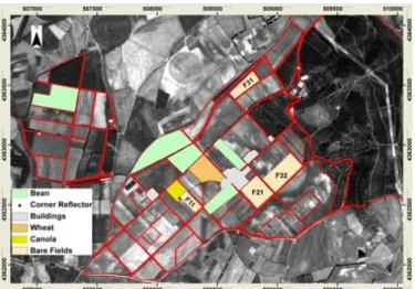
Figure 1 Land-use map of selected reference fields of Azienda San Michele in UTM coordinate system zone 32N (indicating field boundaries, corner reflectors, bare fields and tested crop fields, e.g., bean, wheat and canola fields).

B. Radar Data

A total of 13 dual-polarization ASAR APS images and 11 Radarsat-2 Fine-Quad-Polarization images, including both ascending and descending modes, were acquired over the campaign periods (Table 1). ASAR images covering a swath width of up to 100 km were normalized to a spatial resolution of approximately 30 m. Radarsat-2 images covering a swath width of approximately 25 km were normalized to a spatial resolution of approximately 12.5 m. The radiometric precision is within 0.5 dB in both sensors [24]. An average weekly coverage was guaranteed during the campaign period over the study site.

TABLE 1 RADAR IMAGERY COLLECTION. Date (YYMMDD) Sensor Incidence angle (°) Polarizations 080503 ASAR 23 HH, VV 080522 ASAR 23 HH, VV 080524 Radarsat-2 22 HH,VV, HV, VH 080527 Radarsat-2 21 HH,VV, HV, VH 080528 ASAR 19 HH, VV 080531 ASAR 29 HH, VV 080606 ASAR 41 HH, VV 080613 Radarsat-2 27 HH,VV, HV, VH 080616 ASAR 23 HH, VV 080617 Radarsat-2 22 HH,VV, HV, VH 080624 Radarsat-2 28 HH,VV, HV, VH 090421 ASAR 19 HH, VV 090425 Radarsat-2 22 HH,VV, HV, VH 090427 ASAR 23 HH, VV 090428 Radarsat-2 21 HH,VV, HV, VH 090504 ASAR 29 HH, VV 090513 ASAR 19 HH, VV 090516 ASAR 29 HH, VV 090519 Radarsat-2 22 HH,VV, HV, VH 090522 Radarsat-2 21 HH,VV, HV, VH 090523 ASAR 23 HH, VV 090601 ASAR 23 HH, VV 090612 Radarsat-2 22 HH,VV, HV, VH 090615 Radarsat-2 21 HH,VV, HV, VH C. Field Data

Extensive field measurements were collected from 3rd May to 25th June 2008 and from 21st April to 16th June 2009. The SSM was measured by an FDR (frequency domain reflectometer) at depths of 5 cm and 10 cm (Figure 2) and the gravimetric method was adopted as a reference. The values at each depth were averaged for each reference field to a single representative value for the reference field at the corresponding depth. The SSM measurements were taken each day in accordance with the satellite pass. Surface roughness was measured using the close-range photogrammetric technique with a Rollei 7 camera for each sample point on bare fields [25]. Digital surface models (DSMs) were derived from pairs of photos, where each photo covered a surface area of 1 m by 1 m. The RMS height was calculated from the DSM. Both exponential and Gaussian semivariogram functions were used in ArcGIS 9.x for correlation estimation

from point data of stereo image pairs [26, 27]. Values from different sample points (SPs) were averaged to generate a single representation of each study field. Table 2 demonstrates the minimum and maximum values of field-averaged SSM, RMS height (s) and Gaussian correlation length (l). The SSM at both depths ranged from extremely dry (~3.0 vol. %) to nearly 30 vol. % during the campaign periods. On average, the SSM at a 10 cm depth was 5.9 vol. % higher than the measurement at a 5 cm depth. Tables 3 and 4 showed the in-field variability, i.e., the variability between SPs within a in-field, of these parameters for two sampling dates: 6th June 2008 (a wetter period) and 15th June 2009 (a drier period). Note that: 1) between different reference fields within the experimental farm, the field-averaged SSM can reach a difference higher than 10.0 vol. % and 2) the SSM-values of different sample points showed low variations (standard deviation lower than 4 vol. % for all reference fields).

Figure 2 Comparison of SSM at 5 cm and 10 cm depths in 2008 and 2009 showing an RMSE of 4.3 vol. % and a bias of 5.9 vol. %.

TABLE 2 IN-SITU GEOPHYSICAL CHARACTERISTICS AND MEASURED DATES (YYMMDD). SSM_5 cm (vol. %) SSM_10 cm (vol. %) s (cm) l (cm) Min. Date 1.3 090513 3.1 090615 1.7 090516 15.3 090513 Max. Date 25.6 080606 29.2 090427 3.2 080617 28.2 080503 TABLE 3 IN-FIELD VARIABILITY OF SURFACE GEOPHYSICAL PARAMETERS FOR

6TH

JUNE 2008(MEAN VALUE±STANDARD DEVIATION). Field SSM_5 cm (vol. %) SSM_10 cm (vol. %) s (cm) l (cm) F11 25.6±2.1 25.5±2.8 1.6±0.2 20.3±4.9 F21 11.3±2.5 17.8±2.5 2.0±0.4 17.6±4.8 F31 6.9±0.9 8.3±1.5 1.9±0.1 26.8±14.3

TABLE 4 IN-FIELD VARIABILITY OF SURFACE GEOPHYSICAL PARAMETERS FOR 15TH

JUNE 2009(MEAN VALUE±STANDARD DEVIATION). Field SSM_5 cm (vol. %) SSM_10 cm (vol. %) s (cm) l (cm) F11 10.6±5.3 21.3±4.1 2.1±0.2 20.3±5.2 F21 3.0±1.5 13.5±6.3 1.7±0.3 18.0±5.2 F32 2.6±1.0 3.2±1.2 1.6±0.1 16.0±1.0

III. AIEM

The IEM was developed and introduced by Fung et al. [28, 29]. The IEM has been well described (e.g., [18, 30]) and the equations are not reprinted here. The IEM is a widely used analytical physical model and is known for its comprehensive validity under roughness conditions. Wu and Chen [11] updated and improved the IEM by replacing Fresnel reflection coefficients with a transition function that considers both surface roughness and permittivity. Because both the estimation and sensitivity analysis of the surface roughness information in the backscatter model can be problematic, especially concerning the correlation length l, roughness parameters must be treated carefully. Brogioni et al. [16] assessed the AIEM validity for roughness parameterization resulting in a slight extension from the IEM validity [31]. They found that valid RMS heights and correlation lengths range from ~0.77 to 11.1 cm and ~0.11 to 110 cm, respectively, for the C-band signal of the AIEM.

Baghdadi et al. [19, 22] proposed replacing l with a fitting parameter "Lopt" with a Gaussian function for the IEM. The Lopt depends on a given radar wavelength, incidence angle θ, RMS height s and polarization. The empirical correlation length Loptis expressed as in equations 1-3 for the C-band:

) 1 ( ) 23 . 1 (sin 006 . 3 162 . 0 ) , , (s HH 1.494s L_opt













Note that s is described in cm and θ is described in degrees. Good results were found in [18, 19, 22], where simulated backscattering coefficients and those retrieved from SAR agreed well for soil moistures between 5% and 47%. Equations 1-3 will be applied in this study to measurements collected in a semi-arid environment that is drier than that of the study sites in [18, 19, 22].

IV. MODEL VALIDATION

The empirical correlation length is calculated from the in

situ RMS height and incidence angle in accordance with the

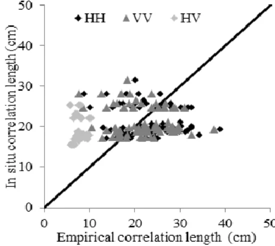
polarization (equations 1-3). The Lopt values were lower in the HV than the HH and VV polarizations. The comparison between in situ l and Lopt showed RMSEs of approximately 7 cm and 12 cm for the co-polarizations (HH and VV) and the cross-polarization, respectively (Figure 3). Moreover, l was larger than Lopt by approximately 2 cm, 1 cm and 11 cm for the HH, VV and HV polarizations, respectively.

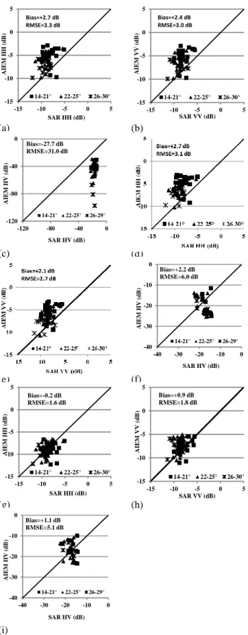
Figure 4 showed a comparison between the backscattering coefficients retrieved from SAR and those simulated from the AIEM, with different ranges of the incidence angle. The simulations were conducted based on SSM_5 cm and SSM_10 cm. The empirical correlation length was also calculated according to equations 1-3. Figures 4a, 4b and 4c were plotted from in situ experiments Gaussian correlation length and SSM_10 cm for the HH, VV and HV polarizations, respectively and were used to exemplify the backscatter simulations from the in situ measurements. Similarly, for the

HH, VV and HV polarizations, Figures 4d, 4e and 4f were plotted simulations from the empirical correlation length and the SSM at 5 cm, while Figures 4g, 4h and 4i were plotted simulations from the empirical correlation length and the SSM at 10 cm. Note that only 33 samples were available for cross-polarization from Radarsat-2 data against 70 samples for HH and VV.

Figure 3 Comparison of empirical correlation length Lopt for the HH, HV and VV polarizations and in situ correlation length l in cm.Each dot represents a correlation value for one reference field and one image acquisition date.

For in situ correlation length l, the backscattering coefficients generated from SSM_10 cm fit the HH and VV polarizations better than did those from SSM_5 cm. For the HV polarization, the selections of l at 5 cm or 10 cm provided similar simulations. By comparing the backscattering coefficients simulated from SSM_5 cm and those retrieved from the SAR imagery, large underestimations of over 14.0 dB and RMSEs over 27.0 dB were found for both the HH and VV polarizations for the Gaussian correlation function. For HV polarization, an underestimation of 31.0 dB and an RMSE exceeding 33.0 dB were observed. Figures 4 a-c showed that the AIEM simulated from SSM_10 cm results in an overestimation of approximately 2.5 dB and an RMSE of approximately 3.1 dB for the HH and VV polarizations, a major improvement. However, a significantly large underestimation of over 27.7 dB and an RMSE of 31.0 dB were found again for the HV polarization.

For the empirical correlation length Lopt, a comparison between figures 4 d-f and 4 g-i showed clear improvement in both RMSEs and bias for the simulations from the SSM_10 cm depth over those from SSM_5 cm. Overestimations of approximately 2.7 dB, 2.1 dB and 2.2 dB and RMSEs of approximately 3.1 dB, 2.7 dB and 6.0 dB were found for the AIEM simulations from SSM_5 cm for the HH, VV and HV polarizations, respectively. For the simulations from SSM_10 cm, the biases were restricted to no more than 1.1 dB and the RMSEs were reduced to 1.6 dB, 1.8 dB and 5.1 dB for the HH, VV and HV polarizations, respectively.

The effect of incidence angle on the performance of the AIEM model was not analyzed because the available samples were acquired mainly with incidence angles between 20° and 30°. The few samples with incidence angles of less than 20° or greater than 30° were not sufficient to analyze the influence of

the incidence angle on the quality of the AIEM simulations. -15 -10 -5 0 5 -15 -10 -5 0 5 A IEM H H (d B ) SAR HH (dB) 14-21° 22-25° 26-30° Bias=+2.7 dB RMSE=3.3 dB (a) -15 -10 -5 0 5 -15 -10 -5 0 5 AIEM V V (d B ) SAR VV (dB) 14-21° 22-25° 26-30° Bias=+2.4 dB RMSE=3.0 dB (b) -120 -80 -40 0 -120 -80 -40 0 AI EM H V (d B ) SAR HV (dB) 14-21° 22-25° 26-29° Bias=-27.7 dB RMSE=31.0 dB (c) (d) (e) -40 -30 -20 -10 0 -40 -30 -20 -10 0 AI EM H V (d B ) SAR HV (dB) 14-21° 22-25° 26-29° Bias=+2.2 dB RMSE=6.0 dB (f) -15 -10 -5 0 5 -15 -10 -5 0 5 AI EM H H (d B ) SAR HH (dB) 14-21° 22-25° 26-30° Bias=-0.2 dB RMSE=1.6 dB (g) -15 -10 -5 0 5 -15 -10 -5 0 5 AI EM V V (d B ) SAR VV (dB) 14-21° 22-25° 26-30° Bias=+0.9 dB RMSE=1.8 dB (h) -40 -30 -20 -10 0 -40 -30 -20 -10 0 A IEM H V (d B ) SAR HV (dB) 14-21° 22-25° 26-29° Bias=+1.1 dB RMSE=5.1 dB (i)

Figure 4 Comparison between backscattering coefficients estimated from the AIEM model and those calculated from the SAR images for the HH, VV and HV polarizations: s and l using in situ SSM_10 cm (a, b, c); s and Lopt using in situ SSM_5 cm (equation 1) (d, e, f); and s and Lopt (equation 1) using in situ SSM_10 cm (g, h, i). Each dot represents a

correlation value for one reference field and one image acquisition date. Bias is defined as AIEM-SAR values.

The better performances of the AIEM based on the SSM at a 10 cm depth could be due to the significant penetration of the radar wave in this semi-arid environment, i.e., the radar signal is more sensitive to deep layers in dry soil.

For a more detailed study of the model performance at different depths, the dataset was separated into two parts: (1) samples with SSM_5 cm < 10 vol. % and (2) samples with SSM_5 cm > 10 vol. %, independent of the SSM at 10 cm. For SSM_5 cm < 10 vol. %, the difference between the AIEM with Lopt and SAR data (bias) decreased from +2.3 dB (SSM_5 cm) to -0.5 dB (SSM_10 cm) for HH, from +1.80 dB (SSM_5 cm) to +0.7 dB (SSM_10 cm) for VV and from -5.4 dB (SSM_5 cm) to -1.1 dB (SSM_10 cm) for HV. For SSM_5 cm > 10%, the bias decreased from +3.4 dB (SSM_5 cm) to +0.3 dB (SSM_10 cm) for HH and from +2.7 dB (SSM_5 cm) to +1.5 dB (SSM_10 cm) for VV. The statistics for HV were not calculated because only 10 samples were available for SSM_5 cm > 10%.

In the totality of samples with all polarizations, the statistics showed that the difference between the AIEM with Lopt and the SAR data decreased from +0.7 dB (SSM_5 cm) to -0.2 dB (SSM_10 cm) for SSM_5 cm < 10 vol. % and from +3.3 dB (SSM_5 cm) to +1.8 dB (SSM_10 cm) for SSM_5 cm > 10 vol. %. The RMSE decreased from 3.7 dB (SSM_5 cm) to 2.4 dB (SSM_10 cm) for SSM_5 cm < 10 vol. % and from 3.7 dB (SSM_5 cm) to 3.2 dB (SSM_10 cm) for SSM_5 cm > 10 vol. %.

V. DISCUSSION AND CONCLUSIONS

This study confirmed the applicability of Lopt in the AIEM model. Moreover, these results showed that the use of Lopt ensures better agreement between the AIEM model and the SAR data when using a dataset acquired in a semi-arid environment with an SSM_10 cm between 3.1 vol. % and 29.2 vol. %. The RMSE was lower for the HH and VV polarizations than for the HV polarizations. However, these results were obtained with fewer samples for HV (33 points for HV and 70 points for HH and VV). This approach can help to minimize the uncertainties introduced by correlation length measurement. Comparably, Huang et al. [14] reported a promising confidence level of approximately 2.0 dB in bias for the AIEM performance in a total of 34 samples, while this study showed a bias within 1.0 dB for HH and VV polarizations from 70 samples and a bias of 1.1 dB for HV polarization from 33 samples. Additional theoretical models may need to be considered to assess the empirical correlation length.

The empirical correlation length solves the scale effect on the parameterizing correlation length. When accurate inversions of both RMS height and SSM from remote sensing-based approaches are available, such as when using full polarimetric SAR [34], the AIEM coupled with Lopt can be used as an operational approach. Promising soil moisture data retrieval from SAR imagery is expected from the use of

empirical correlation length-parameterized AIEM for field-scale purposes in semi-arid environments.

ACKNOWLEDGMENTS

This work was partly financed through the multi-disciplinary, multi-national FP7 project CLIMB (CLimate Induced changes on the hydrology of Mediterranean Basins) and DAAD (German Academic Exchange Service). The authors would like to acknowledge their colleagues from LMU Muenchen, INRS Quebec, University of Cagliari and

Azienda San Michele, who participated in the field campaigns.

REFERENCES

1 Deroin, J.P., Company, A., and Simonin, A.: ‘An empirical model for interpreting the relationship between backscattering and arid land surface roughness as seen with the SAR’, Geoscience and Remote Sensing, IEEE Transactions on, 1997, 35, (1), pp. 86-92

2 Hallikainen, M.T., Ulaby, F.T., Dobson, M.C., Elrayes, M.A., and Wu, L.K.: ‘Microwave Dielectric Behavior of Wet Soil .1. Empirical-Models and Experimental-Observations’, IEEE Transactions on Geoscience and Remote Sensing, 1985, 23, (1), pp. 25-34

3 Oh, Y., Sarabandi, K., and Ulaby, F.T.: ‘An Empirical-Model and an Inversion Technique for Radar Scattering from Bare Soil Surfaces’, Ieee Transactions on Geoscience and Remote Sensing, 1992, 30, (2), pp. 370-381 4 Zribi, M., and Dechambre, M.: ‘A new empirical model to retrieve soil moisture and roughness from C-band radar data’, Remote Sens. Environ., 2003, 84, (1), pp. 42-52

5 Dubois, P.C., Van Zyl, J., and Engman, T.: ‘Measuring Soil-Moisture with Imaging Radars’, IEEE Transactions on Geoscience and Remote Sensing, 1995, 33, (4), pp. 915-926

6 Loew, A., Ludwig, R., and Mauser, W.: ‘Derivation of surface soil moisture from ENVISAT ASAR wide swath and image mode data in agricultural areas’, Ieee Transactions on Geoscience and Remote Sensing, 2006a, 44, (4), pp. 889-899

7 Loew, A., and Mauser, W.: ‘A semiempirical surface backscattering model for bare soil surfaces based on a generalized power law spectrum approach’, Ieee Transactions on Geoscience and Remote Sensing, 2006b, 44, (4), pp. 1022-1035

8 Oh, Y., Sarabandi, K., and Ulaby, F.T.: ‘Semi-empirical model of the ensemble-averaged differential Mueller matrix for microwave backscattering from bare soil surfaces’, Ieee Transactions on Geoscience and Remote Sensing, 2002, 40, (6), pp. 1348-1355

9 Thoma, D.P., Moran, M.S., Bryant, R., Rahman, M., Holifield-Collins, C.D., Skirvin, S., Sano, E.E., and Slocum, K.: ‘Comparison of four models to determine surface soil moisture from C-band radar imagery in a sparsely vegetated semiarid landscape’, Water Resour. Res., 2006, 42, (1), pp. -

10 Fung, A.K., and Pan, G.W.: ‘A scattering model for perfectly conducting random surfaces I. Model development’, International Journal of Remote Sensing, 1987, 8, (11), pp. 1579 - 1593

11 Wu, T.D., and Chen, K.S.: ‘A reappraisal of the validity of the IEM model for backs cattering from rough surfaces’, Ieee Transactions on Geoscience and Remote Sensing, 2004, 42, (4), pp. 743-753

12 Wu, T.D., Chen, K.S., Shi, J.C., Lee, H.W., and Fung, A.K.: ‘A study of an AIEM model for bistatic scattering from randomly rough surfaces’, Ieee Transactions on Geoscience and Remote Sensing, 2008, 46, (9), pp. 2584-2598

13 Song, K.J., Zhou, X.B., and Fan, Y.: ‘Empirically Adopted IEM for Retrieval of Soil Moisture From Radar Backscattering Coefficients’, Ieee Transactions on Geoscience and Remote Sensing, 2009, 47, (6), pp. 1662-1672

14 Huang, S.W., Tsang, L., Njoku, E.G., and Chan, K.S.: ‘Backscattering Coefficients, Coherent Reflectivities, and Emissivities of Randomly Rough Soil Surfaces at L-Band for SMAP Applications Based on Numerical Solutions of Maxwell Equations in Three-Dimensional Simulations’, Ieee Transactions on Geoscience and Remote Sensing, 2010, 48, (6), pp. 2557-2568

15 Chen, K.S., Tzong-Dar, W., Leung, T., Qin, L., Jiancheng, S., and Fung, A.K.: ‘Emission of rough surfaces calculated by the integral equation method with comparison to three-dimensional moment method simulations’,

Geoscience and Remote Sensing, IEEE Transactions on, 2003, 41, (1), pp. 90-101

16 Brogioni, M., Pettinato, S., Macelloni, G., Paloscia, S., Pampaloni, P., Pierdicca, N., and Ticconi, F.: ‘Sensitivity of bistatic scattering to soil moisture and surface roughness of bare soils’, International Journal of Remote Sensing, 2010, 31, (15), pp. 4227-4255

17 Nearing, G.S., Moran, M.S., Thorp, K.R., Collins, C.D.H., and Slack, D.C.: ‘Likelihood parameter estimation for calibrating a soil moisture model using radar bakscatter’, Remote Sens. Environ., 2010, 114, (11), pp. 2564-2574

18 Baghdadi, N., Gherboudj, I., Zribi, M., Sahebi, M., King, C., and Bonn, F.: ‘Semi-empirical calibration of the IEM backscattering model using radar images and moisture and roughness field measurements’, International Journal of Remote Sensing, 2004, 25, (18), pp. 3593-3623

19 Baghdadi, N., Holah, N., and Zribi, M.: ‘Calibration of the Integral Equation Model for SAR data in C-band and HH and VV polarizations’, International Journal of Remote Sensing, 2006a, 27, (4), pp. 805-816 20 Lievens, H., Verhoest, N.E.C., De Keyser, E., Vernieuwe, H., Matgen, P., Alvarez-Mozos, J., and De Baets, B.: ‘Effective roughness modelling as a tool for soil moisture retrieval from C-and L-band SAR’, Hydrol. Earth Syst. Sci., 2011, 15, (1), pp. 151-162

21 Verhoest, N.E.C., Lievens, H., Wagner, W., Alvarez-Mozos, J., Moran, M.S., and Mattia, F.: ‘On the soil roughness parameterization problem in soil moisture retrieval of bare surfaces from synthetic aperture radar’, Sensors, 2008, 8, (7), pp. 4213-4248

22 Baghdadi, N., Abou Chaaya, J., and Zribi, M.: ‘Semiempirical Calibration of the Integral Equation Model for SAR Data in C-Band and Cross Polarization Using Radar Images and Field Measurements’, IEEE Geosci. Remote Sens. Lett., 2011, 8, (1), pp. 14-18

23 Ludwig, R., Roson, R., Zografos, C., and Kallis, G.: ‘Towards an inter-disciplinaryresearchagenda on climatechange, water and security in Southern Europe and neighboring countries’, Environmental Science & Policy, 2011, 14, (7), pp. 794-803

24 Baghdadi, N., Zribi, M., and Delorme, A.: ‘Assessment of the ASAR sensor radiometric quality in comparison to ERS-2 and RADARSAT-1 SAR data’, International Journal of Remote Sensing, 2008, 29, (16), pp. 4653-4665

25 Marzahn, P., and Ludwig, R.: ‘On the derivation of soil surface roughness from multi parametric PolSAR data and its potential for hydrological modeling’, Hydrol. Earth Syst. Sci., 2009, 13, (3), pp. 381-394 26 Merzouki, A., Bannari, A., Teillet, P.M., and King, D.J.: ‘Geostatistical characterization of spatial variability of soil moisture with the help of maps from RADARSAT-1 C-band synthetic aperture radar data’, Can J Remote Sens, 2008, 34, (4), pp. 376-389

27 Curran, P.J.: ‘THE SEMIVARIOGRAM IN REMOTE-SENSING - AN INTRODUCTION’, Remote Sens. Environ., 1988, 24, (3), pp. 493-507 28 Fung, A.K.: ‘Microwave scattering and emission models and their applications’ (Artech House, 1994. 1994)

29 Fung, A.K., Li, Z., and Chen, K.S.: ‘Backscattering from a randomly rough dielectric surface’, Geoscience and Remote Sensing, IEEE Transactions on, 1992, 30, (2), pp. 356-369

30 Baghdadi, N., and Zribi, M.: ‘Evaluation of radar backscatter models IEM, OH and Dubois using experimental observations’, International Journal of Remote Sensing, 2006c, 27, (18), pp. 3831-3852

31 Macelloni, G., Nesti, G., Pampaloni, P., Sigismondi, S., Tarchi, D., and Lolli, S.: ‘Experimental validation of surface scattering and emission models’, Ieee Transactions on Geoscience and Remote Sensing, 2000, 38, (1), pp. 459-469

32 Baghdadi, N., Aubert, M., Cerdan, O., Franchisteguy, L., Viel, C., Martin, E., Zribi, M., and Desprats, J.F.: ‘Operational mapping of soil moisture using synthetic aperture radar data: Application to the touch basin (France)’, Sensors, 2007, 7, (10), pp. 2458-2483

33 Baghdadi, N., Camus, P., Beaugendre, N., Issa, O.M., Zribi, M., Desprats, J.F., Rajot, J.L., Abdallah, C., and Sannier, C.: ‘Estimating Surface Soil Moisture from TerraSAR-X Data over Two Small Catchments in the Sahelian Part of Western Niger’, Remote Sensing, 2011, 3, (6), pp. 1266-1283 34 Hajnsek, I., Pottier, E., and Cloude, S.R.: ‘Inversion of surface parameters from polarimetric SAR’, IEEE Transactions on Geoscience and Remote Sensing, 2003, 41, (4), pp. 727-744