Site-selective isomerization of cyano-substituted butadienes: chemical control of nonadiabatic dynamics

(1)

Supporting Information — Site-selective

isomerization of cyano-substituted butadienes:

Chemical control of nonadiabatic dynamics

Ryan J. MacDonell

†

and Michael S. Schuurman

∗,†,‡

†Department of Chemistry and Biomolecular Sciences, University of Ottawa, D’Iorio Hall, 10 Marie Curie, Ottawa, Ontario, K1N 6N5, Canada.

‡National Research of Council Canada, 100 Sussex Drive, Ottawa, Ontario K1A 0R6, Canada.

E-mail: michael.schuurman@nrc-cnrc.gc.ca

1 Spawning

As per the original definition of FMS on adiabtic surfaces,1 _{a spawning event occurs when}

the dot product of the nonadiabatic coupling vector d and the velocity v exceeds a set threshold. This threshold is chosen such that only sharp peaks in d · v exceed it in a set of test calculations. Thresholds of 0.014, 0.015 and 0.015 a.u. were chosen for BD, 1-CNBD and 2-CNBD, respectively. New trajectories are also required to conserve the classical energy of the nuclear basis, thus their momentum was scaled by the energy difference between states. Cases with kinetic energy less than the potential energy difference are rejected.

Although the choice of spawning is arbitrary and does not necessarily correspond to a change in state population, the choice of spawning criteria given above generally results in population transfer occuring at or near the spawn time. Figure S1 shows the population

(2)

0.0

0.2

0.4

0.6

0.8

1.0 p

c

(a)

0.00

0.05

0.10

0.15 dp

c

/d

t

(d)

0.0

0.2

0.4

0.6

0.8

1.0 p

c

(b)

0.00

0.05

0.10

0.15 dp

c

/d

t

(e)

25

0

25

50

75 t t

spawn

/ a.u.

0.0

0.2

0.4

0.6

0.8

1.0 p

c

(c)

25

0

25

50

75 t t

spawn

/ a.u.

0.00

0.05

0.10

0.15 dp

c

/d

t

(f)

Figure S1: Ground state trajectory populations (a-c) and their time derivatives (d-f) as a function of time from spawn. Plots are given for BD, 1-CNBD and 2-CNBD from top to bottom. Line opacity is proportional to the total population transferred.

(3)

of new trajectories on the ground electronic state and their derivatives as a function of the time difference from tspawn. The opacity for each trajectory is given by the total “population

transferred” of that spawning event. The spawn time occurs within 10 a.u. of the inflection point in all cases, and population changes tend to occur within ∼60 a.u. of the spawning event. Given the relatively slow vibrational periods of the molecules, assigning properties based on the spawn geometry yields nearly identical results to measuring properties weighted by dpc/dt for all times. The former was used for data in Figures 3 and 4. It should be noted

that this assumption is only valid for certain systems, namely those with localized, peaked conical intersection regions (e.g. polar polyenes and small non-polar polyenes).

2 Bootstrap sampling

The standard deviation is a poor measure of the error associated with the mean adiabatic populations ¯p due to the variation between initial conditions. Instead, “bootstrap samples” are generated by sampling the set of initial conditions with replacement, i.e. an initial condition may be included more than once, but the total number of initial conditions remains the same for each sample. Averaging over initial conditions in a sample i generates sample populations pi. The mean values hpi and standard deviations σ can then be calculated from

multiple bootstrap samples. As the number of samples increases, the bootstrap mean hpi converges to the true mean ¯p where each initial condition is included once.2

To avoid storing adiabatic populations for thousands of bootstrap samples, the mean and variance are updated incrementally.3 _{For sample number n, let}

hpin= 1 n n X i=0 pi, (S1) ∆n= n X i=0 (pi− hpin)2. (S2)

(4)

These values are updated by generating a new bootstrap sample pn+1, then en+1 = pn+1− hpin, (S3) hpin+1 = hpin+ en+1 n + 1, (S4) ∆n+1 = ∆n+ en+1(pn+1− hpin+1) . (S5)

Convergence is achieved when max |hpin− ¯p| < δ for all times and states with a set threshold

δ. The standard deviation is then given by σn =

r ∆n

n − 1. (S6)

Only the current values of hpin and ∆n need to be stored, and they are updated until

convergence. We use a convergence threshold of δ = 10−3, requiring roughly 3000–8000 bootstrap samples for each molecule.

(5)

3 Photochemical yield

0

50

100

150 |

C2 C3

| /

°

(a)

40.9%

59.1%

(d)

0

50

100

150 |

C2 C3

| /

°

(b)

40.7%

59.3%

(e)

0

200

400

600 800 1000

t t

spawn

/ fs

0

50

100

150 |

C2 C3

| /

°

(c)

0.0

0.5

1.0 Population / 10

2

49.0%

51.0%

(f)

0.000 0.002 0.004 0.006 0.008

Figure S2: Ground state wavefunction density (a-c) as a function of time from spawn and C2-C3 dihedral angle and (d-f) densities integrated from 200 fs to the end of the simulation.

(6)

4 Potential energy surfaces

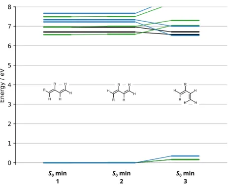
Figure S3: MR-CIS/6-31G* ground state potential energy minima of BD (black), 1-CNBD (green) and 2-CNBD (blue).

Figure S4: MS-CASPT2/cc-pVTZ ground state potential energy minima of BD (black), 1-CNBD (green) and 2-CNBD (blue).

(7)

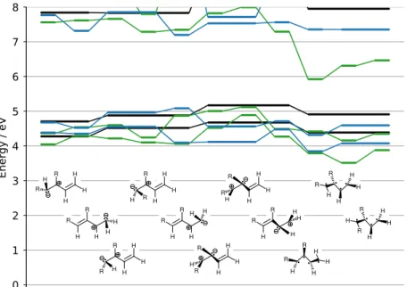
Figure S5: MR-CIS/6-31G* S2-S1 minimum energy conical intersections of BD (black),

1-CNBD (green) and 2-1-CNBD (blue).

Figure S6: MS-CASPT2/cc-pVTZ S2-S1 minimum energy conical intersections of BD

(8)

Figure S7: MR-CIS/6-31G* S1-S0 minimum energy conical intersections of BD (black),

1-CNBD (green) and 2-1-CNBD (blue).

Figure S8: MS-CASPT2/cc-pVTZ S1-S0 minimum energy conical intersections of BD

(9)

Table S1: MR-CIS/6-31G* potential energies of BD critical geometries. Energy / Eh Geometry S0 S1 S2 1, 2 −155.0487659848 −154.8023180095 −154.7929770444 3 −155.0427635433 −154.8070399811 −154.8020210437 C1Tw1 −154.9496358805 −154.8254668870 −154.8254666863 C1Tw2 −154.9321085728 −154.8122623407 −154.8122593724 C1Tw3 −154.9499109734 −154.8297179987 −154.8297177233 H1Br1 −154.8508456793 −154.8508002978 −154.7223639172 H1Br2 −154.8443901889 −154.8440556562 −154.7230354871 R2Br −154.8357835236 −154.8357827967 −154.7201466902 C2Tr −154.8538763952 −154.8538759847 −154.7243602701

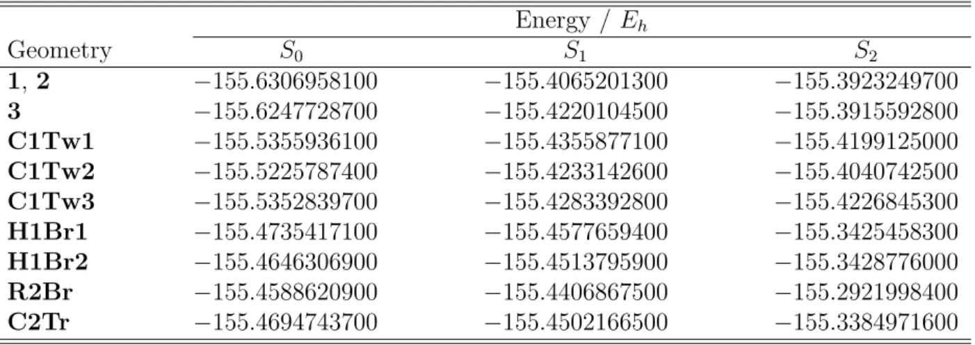
Table S2: MS-CASPT2/cc-pVTZ potential energies of BD critical geometries. Energy / Eh Geometry S0 S1 S2 1, 2 −155.6306958100 −155.4065201300 −155.3923249700 3 −155.6247728700 −155.4220104500 −155.3915592800 C1Tw1 −155.5355936100 −155.4355877100 −155.4199125000 C1Tw2 −155.5225787400 −155.4233142600 −155.4040742500 C1Tw3 −155.5352839700 −155.4283392800 −155.4226845300 H1Br1 −155.4735417100 −155.4577659400 −155.3425458300 H1Br2 −155.4646306900 −155.4513795900 −155.3428776000 R2Br −155.4588620900 −155.4406867500 −155.2921998400 C2Tr −155.4694743700 −155.4502166500 −155.3384971600

(10)

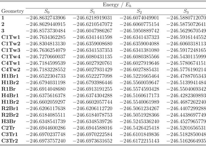
Table S3: MR-CIS/6-31G* potential energies of 1-CNBD critical geometries. Energy / Eh Geometry S0 S1 S2 S3 1 −246.8632743906 −246.6218919031 −246.6074049901 −246.5880712070 2 −246.8629440915 −246.6210547072 −246.6060775154 −246.5875072641 3 −246.8573730484 −246.6047986267 −246.5950889742 −246.5629670549 C1Tw1 −246.7634362285 −246.6341441598 −246.6341437323 −246.5916144552 C1Tw2 −246.8304813130 −246.6359008680 −246.6359004088 −246.6060318113 C1Tw3 −246.7636254079 −246.6341537353 −246.6341381080 −246.5917248165 C1Tw4 −246.7270660037 −246.6080431135 −246.6080385566 −246.5430115999 C4Tw1 −246.7184599539 −246.6027920761 −246.6027919646 −246.5780674151 C4Tw2 −246.7183228552 −246.6027931429 −246.6027885431 −246.5776190214 H1Br1 −246.6522304733 −246.6522277098 −246.5221665464 −246.4788705343 H1Br2 −246.6794031198 −246.6793986446 −246.5560059647 −246.5139941484 R1Br −246.6914048680 −246.6913191255 −246.5574593428 −246.5504069342 H4Br1 −246.6375616378 −246.6374304288 −246.5160617173 −246.4282369893 H1Br2 −246.6602059297 −246.6602057744 −246.5540061989 −246.4687262240 R2Br1 −246.6206117638 −246.6206112720 −246.5061234267 −246.4407299288 R2Br2 −246.6184085511 −246.6184078753 −246.5051928366 −246.4438697749 H3Br −246.6348541739 −246.6348539726 −246.5245336240 −246.4527965779 C2Tr −246.6944600286 −246.6944588016 −246.5426425418 −246.5201656531 C3Tr1 −246.6970237748 −246.6970222584 −246.6101849836 −246.5182850048 C3Tr2 −246.6973757240 −246.6973631652 −246.6172215143 −246.5162664935

(11)

Table S4: MS-CASPT2/cc-pVTZ potential energies of 1-CNBD critical geometries. Energy / Eh Geometry S0 S1 S2 S3 1 −247.7067678600 −247.4903136800 −247.4798788100 −247.4623051100 2 −247.7072183800 −247.4918705700 −247.4803570800 −247.4616745900 3 −247.7000435800 −247.4842104700 −247.4505843400 −247.4458892900 C1Tw1 −247.6101142600 −247.5135896100 −247.4834568900 −247.4605100700 C1Tw2 −247.6726562400 −247.5012213000 −247.4898758400 −247.4714675700 C1Tw3 −247.6102928900 −247.5135540300 −247.4834746900 −247.4604541400 C1Tw4 −247.6259953800 −247.5190032000 −247.5095919400 −247.4374942400 C4Tw1 −247.6133855400 −247.5128161700 −247.5113802700 −247.4875813200 C4Tw2 −247.6132805100 −247.5128360700 −247.5113692600 −247.4871355700 H1Br1 −247.5585597000 −247.5467543900 −247.4293206200 −247.3828396000 H1Br2 −247.5522384900 −247.5382214600 −247.4256642100 −247.3874315900 R1Br −247.5565040800 −247.5512542200 −247.4394207100 −247.4206030400 H4Br1 −247.5496610100 −247.5404505800 −247.4273368100 −247.3695342300 H1Br2 −247.5579315700 −247.5281952800 −247.4372605200 −247.3489481700 R2Br1 −247.5410882600 −247.5232399100 −247.4197465900 −247.3767235800 R2Br2 −247.5275486700 −247.5191587800 −247.4133994100 −247.3688083200 H3Br −247.5503574900 −247.5422009900 −247.4391995700 −247.3854166400 C2Tr −247.5679759800 −247.5448434000 −247.4895202400 −247.3418191700 C3Tr1 −247.5780956400 −247.5543770700 −247.4752856100 −247.3660278200 C3Tr2 −247.5646703400 −247.5473978900 −247.4696391900 −247.3899376100

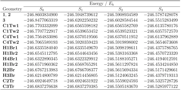
Table S5: MR-CIS/6-31G* potential energies of 2-CNBD critical geometries. Energy / Eh Geometry S0 S1 S2 S3 1, 2 −246.8603834900 −246.5948739612 −246.5908934589 −246.5787428078 3 −246.8477063319 −246.6202250232 −246.6028584544 −246.5515283499 C1Tw1 −246.7703332099 −246.6565598182 −246.6565582769 −246.6135780176 C1Tw2 −246.7707722917 −246.6539653452 −246.6539523321 −246.6357572570 C4Tw1 −246.7564833086 −246.6370519566 −246.6370511952 −246.6137962889 C4Tw2 −246.7065589193 −246.5920359423 −246.5919898002 −246.5654673608 H1Br1 −246.6335584040 −246.6335549670 −246.5098198611 −246.4375786765 H1Br2 −246.6545112795 −246.6544643456 −246.5383163368 −246.4570723320 H4Br1 −246.6322890345 −246.6322329912 −246.5188105271 −246.4194012591 H1Br2 −246.6571960362 −246.6568765291 −246.5611297824 −246.4534244850 R2Br −246.6767213983 −246.6766708377 −246.5615694334 −246.5171429661 H3Br −246.6214800789 −246.6214456805 −246.5124063245 −246.4379719313 C2Tr −246.6924649718 −246.6924631922 −246.5559024593 −246.5325728726 C3Tr −246.6837276638 −246.6837270385 −246.5505183670 −246.5285977122

(12)

Table S6: MS-CASPT2/cc-pVTZ potential energies of 2-CNBD critical geometries. Energy / Eh Geometry S0 S1 S2 S3 1, 2 −247.7045445700 −247.4778939000 −247.4519492000 −247.4484063600 3 −247.6987831900 −247.5064193700 −247.4740609300 −247.4452037800 C1Tw1 −247.6120231400 −247.5245918400 −247.5059554900 −247.4555723600 C1Tw2 −247.6142612600 −247.5170876000 −247.5140581400 −247.4975736800 C4Tw1 −247.6109386400 −247.5103978800 −247.5066845800 −247.4925245900 C4Tw2 −247.6046102500 −247.5035325800 −247.5032914900 −247.4772000500 H1Br1 −247.5434272800 −247.5326866900 −247.4190434700 −247.3251915000 H1Br2 −247.5372499500 −247.5221932000 −247.4159433100 −247.3325593300 H4Br1 −247.5445574100 −247.5383547100 −247.4356873100 −247.3663247200 H1Br2 −247.5540529300 −247.5176837800 −247.4399708500 −247.3337885900 R2Br −247.5532906400 −247.5368529100 −247.4277511500 −247.4209478600 H3Br −247.5400696200 −247.5314285600 −247.4265780400 −247.3780333100 C2Tr −247.5632162900 −247.5458888600 −247.4342062300 −247.4008474600 C3Tr −247.5548263200 −247.5357324900 −247.4342906800 −247.3566684000

5 Molecular geometries

All geometries are given in units of ˚Angstr¨om.

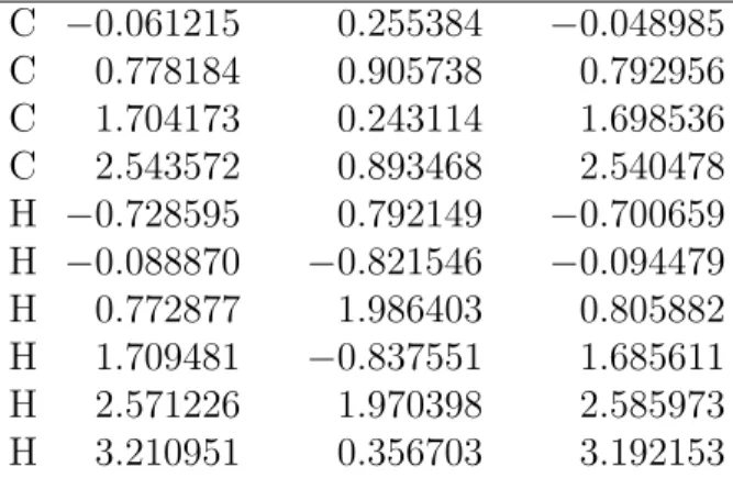
Table S7: MR-CIS optimized geometry of the BD S0 trans minimum (1, 2).

C −0.061215 0.255384 −0.048985 C 0.778184 0.905738 0.792956 C 1.704173 0.243114 1.698536 C 2.543572 0.893468 2.540478 H −0.728595 0.792149 −0.700659 H −0.088870 −0.821546 −0.094479 H 0.772877 1.986403 0.805882 H 1.709481 −0.837551 1.685611 H 2.571226 1.970398 2.585973 H 3.210951 0.356703 3.192153

(13)

Table S8: MR-CIS optimized geometry of the BD S0 cis minimum (3). C −0.108735 0.330951 −0.094729 C 0.763613 0.890255 0.778704 C 1.686701 0.194211 1.680851 C 1.847620 −1.144455 1.817874 H −0.740867 0.947227 −0.710110 H −0.206809 −0.735678 −0.210179 H 0.795802 1.968293 0.829027 H 2.298849 0.835122 2.297489 H 1.278988 −1.856536 1.243208 H 2.561379 −1.542961 2.517748

Table S9: MR-CIS optimized geometry of the BD S2-S1 C1 twist MECI 1 (C1Tw1).

C −1.771535 −1.246620 −0.023181 C −1.444413 0.129504 0.018663 C −0.068024 0.587764 0.028609 C 0.340074 1.965622 −0.005373 H −2.793232 −1.580530 −0.038327 H −0.997381 −1.994505 −0.032692 H −2.223901 0.871766 0.018181 H 0.656683 −0.231675 0.030489 H 0.478275 2.467695 −0.948634 H 0.423848 2.538142 0.903145

Table S10: MR-CIS optimized geometry of the BD S2-S1 C1 twist MECI 2 (C1Tw2).

C 1.447207 −1.402569 1.056560 C 0.405946 −1.179757 0.114504 C −0.684324 −0.247416 0.141261 C −2.002149 −0.472441 −0.259515 H 2.487433 −1.473361 0.755386 H 1.288885 −1.693567 2.096831 H 0.104853 −2.218843 −0.125220 H −0.409066 0.774487 0.366534 H −2.349236 −1.455664 −0.532702 H −2.695176 0.346053 −0.337128

(14)

Table S11: MR-CIS optimized geometry of the BD S2-S1 C1 twist MECI 3 (C1Tw3). C −1.831586 −0.525265 0.194469 C −0.549356 −0.097798 −0.336322 C 0.671398 −0.111266 0.452131 C 1.978019 0.067339 −0.117750 H −2.165698 −1.542577 0.066945 H −2.490360 0.161963 0.700317 H −0.432013 0.155099 −1.386854 H 0.583316 −0.314804 1.505727 H 2.101539 0.232896 −1.173480 H 2.855174 0.070598 0.502653

Table S12: MR-CIS optimized geometry of the BD S1-S0 H1 bridging MECI 1 (H1Br1).

C 1.841822 0.081208 0.057792 C 0.689252 −0.634436 −0.026686 C −0.601895 0.013296 −0.099864 C −1.816004 −0.716548 0.021817 H 2.804941 −0.398401 0.083936 H 1.828613 1.158278 0.096778 H 0.686535 −1.710895 −0.041153 H −0.526662 1.104012 −0.129623 H −2.674613 −0.198314 −0.418122 H −1.816590 −0.006067 0.962993

Table S13: MR-CIS optimized geometry of the BD S1-S0 H1 bridging MECI 2 (H1Br2).

C 1.859253 0.103075 0.022560 C 0.748132 −0.676460 −0.046586 C −0.577449 −0.077563 −0.007071 C −1.853416 −0.695048 0.135308 H 2.839597 −0.319624 0.156861 H 1.788075 1.177231 −0.027326 H 0.825900 −1.750959 0.014039 H −0.550199 0.996762 −0.177030 H −1.828743 −1.660216 0.653989 H −1.411920 −1.164271 −0.851898

(15)

Table S14: MR-CIS optimized geometry of the BD S1-S0 H2 bridging MECI (R2Br). C 1.363655 −1.476755 1.033233 C 0.534891 −0.949371 0.036100 C −0.670060 −0.158282 0.076533 C −1.952814 −0.537649 −0.176377 H 2.387908 −1.747906 0.815252 H 1.012393 −1.807281 2.008700 H 0.204967 −2.070707 0.266985 H −0.474465 0.895795 0.220505 H −2.217818 −1.566881 −0.361516 H −2.737363 0.195240 −0.243732

Table S15: MR-CIS optimized geometry of the BD S1-S0 C2 transoid MECI (C2Tr).

C 1.311740 −0.522258 0.966044 C 0.385161 −0.489594 −0.176401 C −0.147032 0.757933 −0.623599 C −1.486348 0.287422 −0.307643 H 2.173392 0.123071 0.955778 H 1.011290 −0.939779 1.911243 H 0.143552 −1.388069 −0.717179 H 0.236749 1.687881 −0.240237 H −1.988066 −0.424395 −0.939287 H −1.980353 0.592607 0.598953

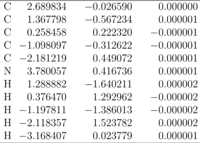
Table S16: MR-CIS optimized geometry of the 1-CNBD S0 trans-trans minimum (1).

C 2.689834 −0.026590 0.000000 C 1.367798 −0.567234 0.000001 C 0.258458 0.222320 −0.000001 C −1.098097 −0.312622 −0.000001 C −2.181219 0.449072 0.000001 N 3.780057 0.416736 0.000001 H 1.288882 −1.640211 0.000002 H 0.376470 1.292962 −0.000002 H −1.197811 −1.386013 −0.000002 H −2.118357 1.523782 0.000002 H −3.168407 0.023779 0.000001

(16)

Table S17: MR-CIS optimized geometry of the 1-CNBD S0 cis-trans minimum (2). C −0.135856 −1.173381 −0.146745 C −0.053411 0.250616 −0.041228 C 0.796001 0.890189 0.810384 C 1.728049 0.232683 1.722031 C 2.533712 0.903062 2.530843 N −0.209025 −2.344566 −0.238832 H −0.710106 0.809965 −0.681941 H 0.779825 1.966727 0.812437 H 1.743734 −0.844082 1.719491 H 2.543999 1.979381 2.559085 H 3.212138 0.397642 3.193968

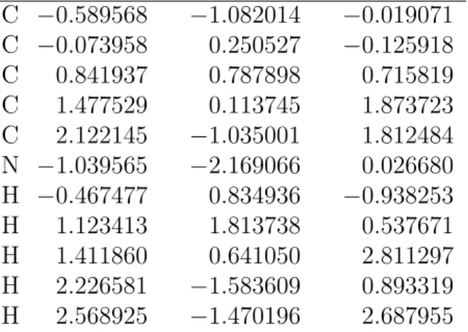
Table S18: MR-CIS optimized geometry of the 1-CNBD S0 cis-cis minimum (3).

C −0.589568 −1.082014 −0.019071 C −0.073958 0.250527 −0.125918 C 0.841937 0.787898 0.715819 C 1.477529 0.113745 1.873723 C 2.122145 −1.035001 1.812484 N −1.039565 −2.169066 0.026680 H −0.467477 0.834936 −0.938253 H 1.123413 1.813738 0.537671 H 1.411860 0.641050 2.811297 H 2.226581 −1.583609 0.893319 H 2.568925 −1.470196 2.687955

Table S19: MR-CIS optimized geometry of the 1-CNBD S2-S1 C1 twist MECI 1 (C1Tw1).

C 0.795804 2.612871 −1.119732 C 0.280518 1.978683 0.024379 C −0.083934 0.562464 0.000674 C −1.402440 0.101669 −0.002818 C −1.748979 −1.215943 −0.016401 N 1.825570 2.686303 −1.852119 H −0.008818 2.609994 0.848880 H 0.720159 −0.155411 −0.056386 H −2.188698 0.838536 0.021491 H −1.004051 −1.991083 −0.042342 H −2.777267 −1.524047 0.009704

(17)

Table S20: MR-CIS optimized geometry of the 1-CNBD S2-S1 C1 twist MECI 2 (C1Tw2). C 2.658087 −1.996892 0.816966 C 1.570311 −1.236078 0.888234 C 0.377534 −1.293179 0.085405 C −0.702220 −0.408576 0.285036 C −1.847549 −0.404591 −0.429181 N 3.722782 −2.706128 0.781331 H 1.656235 −0.493920 1.675818 H 0.318556 −2.037054 −0.688944 H −0.595056 0.320371 1.074125 H −2.016537 −1.104075 −1.229282 H −2.631508 0.300264 −0.223756

C −2.388561 −1.756905 0.071252 C −1.781429 −0.489997 0.117192 C −0.431386 −0.282047 −0.406058 C 0.689687 −0.079247 0.401348 C 1.947916 0.125422 −0.080048 N −2.903588 −2.598910 −0.721557 H −2.266028 0.267563 0.711569 H −0.302722 −0.325828 −1.476892 H 0.541255 −0.071046 1.469033 H 2.150587 0.125529 −1.136142 H 2.776476 0.304876 0.578834

C 2.642135 0.849098 0.695447 C 2.016678 −0.100944 −0.121536 C 0.725297 −0.669515 0.274328 C −0.475641 −0.133249 −0.318782 C −1.777998 −0.213352 0.288910 N 3.142996 1.614448 1.389638 H 2.484999 −0.354341 −1.055839 H 0.648942 −1.275186 1.162954 H −0.377125 0.410976 −1.242760 H −1.904282 −0.624428 1.299739 H −2.660907 0.070302 −0.253411

(18)

Table S23: MR-CIS optimized geometry of the 1-CNBD S2-S1 C4 twist MECI 1 (C4Tw1). C −3.170670 −1.582788 −0.063118 C −1.799508 −1.235738 −0.030925 C −1.402053 0.102898 0.041917 C −0.060550 0.582972 0.100490 C 0.305422 1.938336 −0.044412 N −4.278176 −1.865603 −0.090663 H −1.082192 −2.034097 −0.089353 H −2.187889 0.839799 0.101186 H 0.770852 −0.099948 −0.061696 H 0.361098 2.506226 −1.020017 H 0.626448 2.573172 0.778458

C −2.857064 0.677328 −0.353170 C −1.974069 −0.427776 −0.372864 C −0.700475 −0.336243 0.197319 C 0.285461 −1.366324 0.229978 C 1.466294 −1.311420 1.001323 N −3.573338 1.568461 −0.337939 H −2.331510 −1.343093 −0.808519 H −0.421418 0.620325 0.611012 H 0.024394 −2.379245 −0.070119 H 1.534624 −1.483299 2.116195 H 2.457423 −1.145108 0.585387

Table S25: MR-CIS optimized geometry of the 1-CNBD S1-S0 H1 bridging MECI 1

(H1Br1). C −2.906004 0.012653 −0.830780 C −1.776645 −0.553291 −0.155878 C −0.512721 0.107111 −0.156281 C 0.717304 −0.619057 −0.033122 C 1.902790 0.029501 0.144966 N −3.828865 0.388718 −1.386835 H −1.860764 0.062944 0.874069 H −0.407248 1.190536 −0.090163 H 0.664094 −1.691435 −0.108461 H 1.943501 1.102092 0.239503 H 2.835775 −0.504295 0.187598

(19)

Table S26: MR-CIS optimized geometry of the 1-CNBD S1-S0 H1 bridging MECI 2 (H1Br2). C −2.093289 −1.761498 0.492156 C −1.798453 −0.518754 −0.136539 C −0.495926 0.033859 −0.087643 C 0.778583 −0.653261 −0.090617 C 1.908121 0.062629 0.134371 N −2.420185 −2.733307 1.035999 H −1.318684 −0.913118 −1.120836 H −0.399827 1.114832 −0.141666 H 0.785712 −1.730669 −0.107528 H 1.888813 1.139361 0.162155 H 2.852423 −0.417321 0.321484

Table S27: MR-CIS optimized geometry of the 1-CNBD S1-S0 R1 bridging MECI (R1Br).

C 1.487555 −0.846603 −1.044237 C 1.517970 −0.583923 0.282284 C 0.319103 0.177172 −0.042397 C −1.035834 −0.373060 −0.076021 C −2.093726 0.424847 −0.073239 N 1.125492 −0.728552 −2.206073 H 1.970051 −1.004994 1.147758 H 0.392420 1.241793 −0.232795 H −1.130385 −1.441661 −0.005639 H −1.996605 1.494147 −0.145207 H −3.092103 0.036728 0.010894

(H4Br1). C 3.133477 −0.598549 −0.062397 C 1.856423 0.053081 −0.040089 C 0.680554 −0.641046 0.038257 C −0.595076 0.031550 0.104510 C −1.810432 −0.698094 0.011123 N 4.154225 −1.098790 −0.081444 H 1.870845 1.128299 −0.079824 H 0.670487 −1.717141 0.058983 H −0.526176 1.121780 0.111280 H −1.769014 −0.019488 −1.006519 H −2.704012 −0.167452 0.348955

(20)

Table S29: MR-CIS optimized geometry of the 1-CNBD S1-S0 H4 bridging MECI 2 (H4Br2). C 3.169787 −0.527616 0.136100 C 1.871922 0.044190 −0.011619 C 0.738281 −0.712934 −0.114341 C −0.568981 −0.080119 −0.024248 C −1.825537 −0.689467 0.207512 N 4.229194 −0.979788 0.251508 H 1.820894 1.119982 −0.017007 H 0.798697 −1.788966 −0.092629 H −0.546993 0.991891 −0.193851 H −1.838951 −1.687743 0.644410 H −1.420732 −1.063342 −0.846343

Table S30: MR-CIS optimized geometry of the 1-CNBD S1-S0H2 bridging MECI 1 (R2Br1).

C 2.713621 −1.848863 0.776282 C 1.342434 −1.476098 1.008991 C 0.570618 −0.894607 −0.018160 C −0.661071 −0.140663 0.070363 C −1.933981 −0.561080 −0.148938 N 3.794965 −2.160797 0.612878 H 0.954785 −1.786697 1.973888 H 0.171683 −2.074708 0.189903 H −0.484323 0.916109 0.211359 H −2.167580 −1.596872 −0.339008 H −2.747060 0.142027 −0.173446

Table S31: MR-CIS optimized geometry of the 1-CNBD S1-S0H2 bridging MECI 2 (R2Br2).

C 0.840096 −1.936294 2.321140 C 1.338068 −1.500478 1.029068 C 0.571289 −0.879856 0.019346 C −0.662229 −0.126846 0.066388 C −1.931558 −0.562174 −0.147343 N 0.466959 −2.229553 3.354515 H 2.363552 −1.777415 0.836780 H 0.169556 −2.068659 0.163781 H −0.490300 0.936170 0.155805 H −2.160652 −1.607488 −0.282249 H −2.745754 0.136172 −0.221070

(21)

Table S32: MR-CIS optimized geometry of the 1-CNBD S1-S0 H3 bridging MECI (H3Br). C −2.992557 0.475228 −0.299530 C −1.969709 −0.520189 −0.235198 C −0.681699 −0.195903 0.109651 C 0.470784 −1.026819 0.083119 C 1.412210 −1.438632 1.035204 N −3.816863 1.260441 −0.344386 H −2.253654 −1.526255 −0.490371 H −0.460127 0.837845 0.327354 H 0.107961 −2.159180 0.387514 H 2.412579 −1.717216 0.732373 H 1.159241 −1.679473 2.064302

Table S33: MR-CIS optimized geometry of the 1-CNBD S1-S0 C2 transoid MECI (C2Tr).

C 0.746298 −1.851081 2.112188 C 0.953061 −1.016163 0.992466 C 0.271924 −1.236122 −0.288815 C −0.700387 −0.219411 −0.118124 C −2.116781 −0.565467 −0.142166 N 0.590861 −2.557383 3.024251 H 1.519198 −0.115157 1.153639 H −0.038973 −2.228635 −0.564846 H −0.376829 0.796179 0.042426 H −2.459863 −1.402705 0.437847 H −2.720583 −0.258765 −0.980443

Table S34: MR-CIS optimized geometry of the 1-CNBD S1-S0C3 transoid MECI 1 (C3Tr1).

C −2.880344 −0.125542 −1.197741 C −2.092068 −0.579329 −0.124718 C −0.727038 −0.095279 0.040543 C 0.285233 −0.958860 −0.435820 C 1.075918 −1.125775 0.764034 N −3.532139 0.266359 −2.079707 H −2.390763 −1.482540 0.373744 H −0.472409 0.819176 0.549206 H 0.050040 −1.773062 −1.096464 H 1.487434 −0.261213 1.256124 H 1.037555 −2.040256 1.331982

(22)

Table S35: MR-CIS optimized geometry of the 1-CNBD S1-S0C3 transoid MECI 2 (C3Tr2). C −2.566492 −1.568401 0.731475 C −2.104201 −0.496610 −0.052258 C −0.719854 −0.058459 0.039745 C 0.244929 −0.986468 −0.418721 C 1.061294 −1.129232 0.762356 N −2.955675 −2.441950 1.396185 H −2.713250 −0.173676 −0.879760 H −0.411442 0.871203 0.488670 H −0.048689 −1.827933 −1.019457 H 1.504926 −0.259336 1.215612 H 1.007723 −2.023320 1.360712

Table S36: MR-CIS optimized geometry of the 2-CNBD S0 trans minimum (1, 2).

C −1.756856 −0.659866 −0.000001 C −0.596775 0.044967 0.000000 C 0.732306 −0.600965 0.000001 C 1.888822 0.035939 −0.000001 C −0.653764 1.484496 0.000001 N −0.690521 2.660076 0.000003 H −2.713044 −0.168640 −0.000001 H −1.742496 −1.735643 0.000000 H 0.710116 −1.677587 0.000003 H 2.816658 −0.506130 −0.000001 H 1.955480 1.109353 −0.000003

Table S37: MR-CIS optimized geometry of the 2-CNBD S0 cis minimum (3).

C −1.799524 −0.645493 −0.000004 C −0.617802 0.016763 −0.000000 C 0.732963 −0.589379 −0.000007 C 1.018988 −1.914705 0.000006 C −0.632464 1.445276 0.000011 N −0.622078 2.603666 0.000021 H −2.730524 −0.109732 0.000005 H −1.844537 −1.718840 −0.000015 H 1.549863 0.111724 −0.000022 H 2.040993 −2.248355 0.000001 H 0.257277 −2.675006 0.000023

(23)

Table S38: MR-CIS optimized geometry of the 2-CNBD S2-S1 C1 twist MECI 1 (C1Tw1). C 0.229584 2.049547 0.001871 C −0.059888 0.615390 −0.000175 C −1.413215 0.107024 −0.001289 C −1.756897 −1.266558 −0.003809 C 1.010826 −0.319560 −0.000566 N 1.922458 −1.047729 −0.000813 H 0.689762 2.423488 −0.902371 H 0.688222 2.420942 0.907823 H −2.183128 0.857570 −0.000114 H −2.788359 −1.566050 −0.004352 H −1.004144 −2.034112 −0.005136

C 1.480630 −1.337981 1.014580 C 0.234657 −1.376347 0.281881 C −0.721444 −0.297496 0.200104 C −1.994321 −0.364278 −0.355772 C 0.044250 −2.693027 −0.150920 N −0.041927 −3.813577 −0.483719 H 2.436156 −1.204659 0.524809 H 1.530561 −1.522825 2.080278 H −0.397341 0.641859 0.620308 H −2.627531 0.503466 −0.350428 H −2.376150 −1.272543 −0.787355

C 0.346617 2.004460 −0.022195 C −0.123243 0.693254 0.017365 C −1.464648 0.181774 0.046550 C −1.606229 −1.246116 0.089758 C 0.839115 −0.389010 0.034029 N 1.538920 −1.315530 0.049878 H 1.402388 2.198800 −0.039911 H −0.335706 2.834703 −0.035319 H −2.348195 0.797952 0.041512 H −1.682457 −1.870952 −0.797376 H −1.657498 −1.818779 1.013197

(24)

Table S41: MR-CIS optimized geometry of the 2-CNBD S2-S1 C4 twist MECI 2 (C4Tw2). C −1.994390 −0.403264 −0.382713 C −0.712595 −0.351157 0.152810 C 0.279389 −1.395887 0.224032 C 1.463668 −1.230147 0.984132 C −0.229323 0.928837 0.628668 N 0.228280 1.886769 1.041255 H −2.627259 0.463282 −0.349751 H −2.394331 −1.324243 −0.767129 H −0.012588 −2.433437 0.100256 H 1.550083 −1.245762 2.117033 H 2.453908 −1.116596 0.548141

(H1Br1). C −1.754736 −0.791762 0.167362 C −0.584113 0.002146 −0.003012 C 0.728489 −0.609404 −0.000883 C 1.901264 0.080113 0.015333 C −0.605037 1.472587 −0.081086 N −0.667467 2.603107 −0.175859 H −2.676217 −0.303671 −0.170727 H −1.767504 −0.084333 1.161713 H 0.708801 −1.685038 −0.006157 H 2.841219 −0.442316 −0.005798 H 1.933106 1.155677 0.042757

(H1Br2). C −1.842147 −0.695637 0.164194 C −0.586782 −0.044720 0.045248 C 0.756853 −0.630417 −0.038939 C 1.903057 0.091561 0.023158 C −0.634083 1.401315 −0.080228 N −0.673266 2.551303 −0.208788 H −1.796721 −1.711490 0.562507 H −1.349482 −1.031791 −0.863681 H 0.790747 −1.707481 −0.034166 H 2.855699 −0.403623 0.085040 H 1.902145 1.167313 0.035975

(25)

Table S44: MR-CIS optimized geometry of the 2-CNBD S1-S0 H4 bridging MECI 1 (H4Br1). C −1.730500 −0.668597 −0.049986 C −0.563969 0.042437 0.020426 C 0.728317 −0.613378 0.106732 C 1.948848 0.096263 0.000022 C −0.621177 1.493272 0.021194 N −0.745040 2.620714 0.026914 H −2.687129 −0.180220 −0.081539 H −1.709528 −1.744211 −0.067098 H 0.636397 −1.700245 0.143316 H 1.941495 −0.605323 −0.994967 H 2.823496 −0.430487 0.389329

(H4Br2). C −1.737085 −0.687205 0.010185 C −0.622672 0.094792 −0.050046 C 0.712870 −0.522917 −0.010757 C 1.986849 0.061700 0.133105 C −0.730804 1.527448 0.015431 N −0.804507 2.680805 0.041344 H −2.718004 −0.266790 0.137083 H −1.649397 −1.758136 −0.044228 H 0.655185 −1.593524 −0.180149 H 2.054274 1.046153 0.594060 H 1.538698 0.472944 −0.884624

Table S46: MR-CIS optimized geometry of the 2-CNBD S1-S0 R2 bridging MECI (R2Br).

C 1.407936 −1.543479 0.892778 C 0.084501 −1.241828 0.376216 C −0.827060 −0.151065 0.188970 C −2.066283 −0.214187 −0.357631 C 0.211395 −2.582171 0.172381 N 0.829014 −3.617407 0.240210 H 2.291515 −1.473105 0.278306 H 1.574505 −1.791167 1.929162 H −0.455564 0.802530 0.529266 H −2.665450 0.673677 −0.449414 H −2.486517 −1.140135 −0.713637

(26)

Table S47: MR-CIS optimized geometry of the 2-CNBD S1-S0 H3 bridging MECI (H3Br). C −1.953690 −0.545712 −0.169919 C −0.661936 −0.160270 0.076990 C 0.550390 −0.950754 0.016490 C 1.366066 −1.473951 1.038760 C −0.408100 1.256838 0.283289 N −0.204713 2.357266 0.476277 H −2.740854 0.180512 −0.248875 H −2.194301 −1.581244 −0.340398 H 0.128900 −2.107091 0.181477 H 2.395535 −1.730502 0.832572 H 0.986958 −1.820842 1.995885

C −1.560288 −0.660640 0.217686 C −0.577256 0.168815 −0.487767 C 0.569179 −0.634809 −0.295475 C 1.790470 −0.080503 0.285611 C −0.578096 1.585177 −0.423536 N −0.612787 2.745706 −0.415880 H −1.764494 −0.490000 1.260054 H −1.868133 −1.599474 −0.208048 H 0.516730 −1.668141 −0.591207 H 2.665105 0.014401 −0.336547 H 1.718055 0.576732 1.132971

C −2.049167 −0.719305 −0.279523 C −0.698568 −0.183816 −0.139414 C 0.383291 −1.085495 −0.378673 C 1.080437 −1.068029 0.907336 C −0.483693 1.181004 0.235813 N −0.349453 2.298806 0.513937 H −2.612078 −0.503209 −1.171772 H −2.312411 −1.596529 0.281264 H 0.186566 −1.998973 −0.908950 H 1.604483 −0.182840 1.223209 H 0.814618 −1.774712 1.677427

(27)

References

(1) Ben-Nun, M.; Quenneville, J.; Mart´ınez, T. J. Ab Initio Multiple Spawning: Photochem-istry from First Principles Quantum Molecular Dynamics. J. Phys. Chem. A 2000, 104, 5161–5175.

(2) Efron, B. Bootstrap methods: Another look at the Jackknife. Ann. Stat. 1979, 7, 1–26. (3) West, D. H. D. Updating Mean and Variance Estimates: An Improved Method. Comm.