Anti-jamming MTI radar using variable pulse-codes

Anti-jamming MTI Radar using Variable Pulse-Codes*

Kenny Lin

B.S. Electrical Engineering

U.S. Naval Academy, 2000

Submitted to the Department of Electrical Engineering and Computer Science in partial fulfillment of the requirements for the degree of

Master of Science in Electrical Engineering and Computer Science at the

MASSACHUSETTS INSTITUTE OF TECHNOLOGY

May 2002

@

BARKER

OF TECHNOLOGY

JUL 3 12002

LIBRARIES

The author hereby grants to MIT permission to reproduce and distribute publicly paper and electronic copies of this thesis document in whole or in part.

A u th o r ... I ... .... ...

Department of Electrical Engineering an4 Computer Science May 24, 2002 Certified by...

(raf C. Robey

Associate Group Leader, Group 101 incoln Laboratory

.<Thesis Supe isor

Certified by ... _L~-~c~

~Davi

*This work was sponsored by the Department of the Navy and the Department of the Air Force under Contract F19682-00-C-0002. Opinions, interpretations, conclusions, and recommendations are those of the

Anti-jamming MTI Radar using Variable Pulse-Codes

by

Kenny Lin

Submitted to the Department of Electrical Engineering and Computer Science on May 24, 2002, in partial fulfillment of the

requirements for the degree of

Master of Science in Electrical Engineering and Computer Science

Abstract

A pulsed Doppler radar is vulnerable to advanced repeat-back jamming techniques. Rapidly

advancing technology producing inexpensive, high performance commercial off-the-shelf

(COTS) components enable the construction of an electronic countermeasure (ECM)

sys-tem capable of exploiting this vulnerability. This thesis addresses this threat by examining the nature of this vulnerability and developing a modification to the pulsed Doppler/MTI radar system.

Pulsed Doppler radar systems use pulse compression waveforms such as pseudonoise

(PN) coded binary phase-modulated sequences. Repeat-back jamming listens, stores, and

repeats back the radar's transmitted signal to block out all other return signals. If a different PN-code is used for each pulse, the radar receiver will be minimally affected by the jamming. However, a varying PN code creates range sidelobe variation that degrades the integrated signal-to-clutter ratio by a factor of ,1 where N is the code length. This severely limits the ability to perform Doppler and Moving-Target Indication (MTI) processing for clutter suppression on the radar return.

To recover this performance loss several receiver filtering and digital signal processing techniques are tested. PN code selection for optimum filter performance is explored resulting in a 7-dB signal-to-clutter performance recovery for a 32-bit code. Digital pulse compression, matched filtering, and adaptive digital equalization filtering methods are applied to the radar return to equalize differences created by variable PN codes. Different equalization algorithms with various subsets of PN-codes are presented and simulated with data sets modelled after existing radar systems. Successful correction reduces clutter, minimizes the performance degradation to MTI due to variable pulse-codes, and resists some types of DRFM jamming.

Thesis Supervisor: Frank C. Robey Title: Associate Group Leader, Group 101 MIT Lincoln Laboratory

Thesis Supervisor: David H. Staelin Title: Professor

Acknowledgments

First and foremost, I would like to thank my advisor, Dr. Michael A. Koerber, for his time spent teaching and advising me at MIT Lincoln Laboratory. It is through his mentorship, tireless tutelage and fine example that I have learned so much about signal processing and engineering research. I would like to thank my thesis supervisors Dr. David H. Staelin and Dr. Frank C. Robey for their guidance and contribution to my education. I would like to thank my friends and staff members at Lincoln Laboratory for their assistance and for making my time here much more enjoyable. Finally, I would like to thank my girlfriend, Yingli Zhu, and my family, Chiun-wen, Su-ching, and Frank for their love and support in all my endeavors.

Contents

1 Introduction

1.1 Pulsed Doppler Radar ....

1.2 MTI Radar ...

1.3 Electronic Countermeasures

1.4 Variable Pulse-Code Radar

1.5 Performance Metrics . . . . .

1.6 Contributions of this Thesis

2 Radar System Simulation

2.1 Radar System Model . . . . .

2.2 Target Model . . . .

2.3 Environmental Model . . . .

2.3.1 Noise Model . . . .

2.3.2 Clutter Model . . . . 2.3.3 Jamming Model . . .

2.4 Return Processing Model

2.4.1 Pulse Compression

2.4.2 Matched Filtering

2.4.3 Weighting . . . .

2.4.4 Doppler Processing . .

2.4.5 MTI Implementation.

2.4.6 Adaptive Digital Equalization Filtering

2.5 Simulation Output . . . . 9 10 10 10 11 11 12 13 15 16 17 17 18 19 22 22 24 24 26 28 30 . . . . 31 . . . . . . . . . . . . . . . . . . . . . . . . . . . . . . . . . . . . . . . . . . . . . . . .

3 Variable Pulse Code Radar 32

3.1 Doppler Degradation ... 32

3.1.1 Target Effects ... ... ... . ... .. .. .... . 34

3.1.2 Clutter Effects . . . . 36

4 Pulse Compression Filtering 43 4.1 Matched Filter Waveforms . . . . 43

4.1.1 Sidelobe Reduction . . . . 44

4.2 Pulse Compression Waveforms . . . . 46

4.2.1 Pulse Compression Filters . . . . 48

4.3 Doppler and MTI Performance . . . . 51

4.3.1 SN R Loss . . . . 54

5 Adaptive Digital Equalization Filtering 56 5.1 Filter Implementation . . . . 56

5.1.1 Time Domain Implementation . . . . 57

5.1.2 Frequency Domain Implementation . . . . 57

5.2 Equalization Strategies . . . . 57

5.3 Doppler and MTI Performance . . . . 60

5.3.1 SN R Loss . . . . 61

6 Anti-Jamming Performance 62

List of Tables

List of Figures

2-1 Radar Simulation Application GUI . . . .

2-2 _{Simulation Flow and System Block Diagram . . . .}

2-3 Radar System Variables . . . .

2-4 Target Component Magnitude and Phase . . . .

2-5 Target Variables . . . .

2-6 Environment Variables . . . .

2-7 Complex Gaussian "White" Noise Component . . . .

2-8 Clutter Component . . . .

2-9 Repeat-Back Jammer Block Diagram . . . .

2-10 False Targets Created by Repeat-Back Jamming . . . . 2-11 MTI Filtered Return with Repeat-Back Jamming . . . . 2-12 Return Processing Variables . . . .

2-13 Matched Filtering vs. Pulse Compression for a 32-Bit PN Code

2-14 Matched Filter Output with Taylor Weighting . . . .

2-15 Matched Filter Output Weighting Comparison . . . . 2-16 Target and Clutter Comparison for Doppler Processing . . . . . 2-17 Doppler Processed Radar Return . . . . 2-18 MTI Filter Impulse and Frequency Response . . . . 2-19 MTI Processed Radar Return . . . .

2-20 Plotting Options . . . . . . . . 14 . . . . 15 . . . . 15 . . . . 16 . . . . 17 . . . . 18 . . . . 19 . . . . 20 . . . . 20 . . . . 21 . . . . 22 . . . . 23 . . . . 25 . . . . 26 . . . . 27 . . . . 29 . . . . 29 . . . . 30 . . . . 31 . . . . 31

3-1 Constant and Variable Pulse-Code Comparison . . . .

3-2 Matched Filter Output and Doppler Spectrum for a Constant Pulse-Code

3-3 Matched Filter Output and Doppler Spectrum for Variable Pulse-Codes

3-4 Variable Pulse-Code Radar Doppler Return without Clutter . . . .

32 33

. 33

3-5 Variable Pulse-Code Radar Doppler Return with Clutter . . . . 37

3-6 Constant Pulse-Code Radar Doppler Return Profile . . . . 42

3-7 Variable Pulse-Code Radar Doppler Return Profile . . . . 42

4-1 Variable Pulse-Code Radar Doppler Return using Random Codes . . . . 45

4-2 Variable Pulse-Code Radar Doppler Return using ±3 Codes . . . . 45

4-3 Mean and Variance of Random and ±3 32-bit PN Codes . . . . 46

4-4 Variable Pulse-Code Doppler Radar Showing Partial Effectiveness . . . . . 47

4-5 Variable Pulse-Code MTI Radar Showing Partial Effectiveness . . . . 48

4-6 Time Response of Reciprocal Spectrum . . . . 49

4-7 Time Response of Reciprocal Spectrum - Nearest Root Inside Unit Circle 50 4-8 Time Response of Reciprocal Spectrum - Nearest Root Outside Unit Circle 51 4-9 Doppler Processing with ±3 Variable Pulse-Codes, Pulse Compression . . 52

4-10 MTI Processing with ±3 Variable Pulse-Codes, Pulse Compression . . . . . 52

4-11 Pulse Compression and MTI Filtered Spectrum Profile -Constant Pulse-Code 53 4-12 Pulse Compression and MTI Filtered Spectrum Profile -Variable Pulse-Codes 53 4-13 Matched Filter and MTI Filtered Spectrum Profile . . . . 54

4-14 Pulse Compression and MTI Filtered Spectrum Profile . . . . 55

5-1 Adaptive Equalization Filter System . . . . 57

5-2 _{Variable Pulse-Code Doppler Radar with Flat Spectrum Equalization Filtering 58} 5-3 Variable Pulse-Code MTI Radar with Flat Spectrum Equalization Filtering 59 5-4 Pulse Compression versus Flat Spectrum Equalization . . . . 59

5-5 Variable Pulse-Code MTI Radar with 1st Pulse Equalization Filtering . . . 60

6-1 Constant Pulse-Code MTI Radar in Repeat-Back Jamming Environment . 62 6-2 Variable Pulse-Code MTI Radar in Repeat-Back Jamming Environment . . 63

Chapter 1

Introduction

Radar systems in hostile environments face the challenge of detecting targets in the midst of noise, clutter, and jamming. The magnitudes of these interference signals are typically many times that of the target signal. Many techniques have been developed to mitigate this interference and extract the target's parameters.

Two classes of radar systems designed for this purpose are the moving target indication (MTI) radar and the pulsed Doppler (PD) radar. Both systems utilize the Doppler effect to separate moving targets from relatively stationary clutter. Clutter typically consists of unwanted radar reflections from the sea, terrain, weather, or chaff.

MTI and PD radars are widely used and play a critical role in many modern radar systems. Civilian systems rely on MTI and PD radar for air surveillance, especially in bad weather. Military applications include the detection of low flying aircraft or missiles from shipboard and airborne radar platforms.

Military radar systems often operate in hostile environments and may be targeted by electronic countermeasures (ECM) such as repeat-back or digital radio-frequency memory (DRFM) jamming. DRFM jamming captures radar signals to amplify and repeat-back to the radar to flood the receiver with erroneous data. Advances in technology have made inexpensive, high-performance radio frequency parts available so that a DRFM jamming system can easily be developed to blind a PD radar. This thesis addresses this threat

by examining the nature of this vulnerability and developing a modification to the pulsed

1.1

Pulsed Doppler Radar

Pulsed Doppler (PD) radar uses Doppler frequencies to determine a target's range rate by analyzing the return from two or more transmitted pulses. Because of the Doppler effect, the radar return of a moving object will be shifted in frequency relative to the frequency of the transmitted signal and stationary objects. PD radars use this difference in frequency to detect moving objects and determine their relative speeds [12]. Using this technique, a moving object with a return signal completely obscured by clutter and noise may still be detected after Doppler processing if its frequency exceeds the frequency range occupied

by the clutter return. The radar system assumed in this thesis is a shipboard or

ground-based pulsed Doppler/MTI radar system with a phased array of antennas that transmits a series of narrow band, beam-formed pulses. The transmitter will use binary phase encoded waveforms [12].

1.2

MTI Radar

Moving Target Indication (MTI) Radar is an older system that uses delay-line cancellers to filter out clutter. The current radar return is compared with previous returns to isolate dif-ferences. The relatively stationary clutter is subtracted out and moving targets remain [11].

A newer implementation of MTI modifies the pulsed Doppler radar return by adding a notch

filter around the Doppler frequencies of the clutter in order to improve the signal-to-clutter ratio [13, 6]. This is the implementation used in this thesis.

1.3

Electronic Countermeasures

In addition to noise and clutter, radar systems in hostile environments may encounter jam-ming. Jamming, or electronic countermeasures (ECM), is an effort by enemy systems to degrade the capability of friendly radar systems. It can be passive, in the form of chaff and decoys, or active, in the form of electromagnetic (EM) transmissions with the intent to deceive or confuse a radar. Electronic counter-countermeasures (ECCM) are efforts by

friendly systems to counter enemy ECM. ECM and ECCM are elements of electronic warfare (EW) [10]. As military forces become more dependent on electromagnetic systems, EW has become crucial on the battlefield. The variable pulse-code modification to the radar system proposed in this thesis can be considered an ECCM system.

1.4

Variable Pulse-Code Radar

PD and MTI radars are susceptible to deceptive ECM (DECM) repeaters. This type of active jamming system, also known as a repeat-back or DRFM jammer, records and repeats back a radar's transmitted waveform to flood the receiver with erroneous data [10]. A possible counter to this system is to use non-repetitive waveforms within each coherent processing interval (CPI) by varying the waveform transmitted by each pulse. If there is little correlation between the current and previous waveform, the signal transmitted by the DRFM jammer will be processed as noise and have minimal effect on the radar return.

If a different pseudo random or pseudonoise (PN) code [3] is used for each pulse, the radar receiver will be minimally affected by the jamming. However, when the return signal is Doppler processed, any variation in the filtered output from these PN codes will degrade the integrated signal-to-clutter ratio. The energy no longer falls in a single Doppler bin after processing. This will be described in detail in Section 3.1. The strength of the clutter signal is amplified and the target signal can be obscured. This severely limits the ability to perform Doppler and MTI processing on the radar return when different PN codes are used within a CPI.

1.5

Performance Metrics

Radar system performance will be measured by the ability of the radar to detect a target obscured by interference. The strength of the target's signal-to-noise and signal-to-clutter ratios will be mathematically predicted and empirically verified. This allows us to quantify performance degradation or improvement as we modify the system.

1.6

Contributions of this Thesis

There is a significant performance loss in the ability to Doppler process or apply an MTI filter to the return of a variable pulse-code radar. The performance loss was found to be the result of clutter range sidelobe variation. This thesis presents several receiver filtering meth-ods by which this performance may be recovered. A simulation framework and graphical user interface created for PD and MTI radar simulation will be presented. The signal-to-clutter ratio degradation of the return when using variable code sets and matched filtering will be quantified. Pulse compression is explored as an alternative. However, pulse com-pression filters do not meet the signal-to-noise ratio (SNR) optimality criteria of matched filtering. Adaptive digital equalization filtering methods are applied to the matched filter output to attempt to recover PD and MTI performance. The SNR loss of applying the equalization filter will be compared with the SNR loss of a pulse compression filter. Pulse code selection for maximum filter performance and weighting techniques for further per-formance improvements will be explored. Finally, the effect of jamming on constant and variable pulse-code sequences will be shown to test the success of the variable pulse-code radar solution to repeat-back jamming.

Chapter 2

Radar System Simulation

The variable pulse-code Doppler/MTI radar system and all return data were simulated in Matlab®. The time and cost required to perform the modifications required to test this system in hardware were impractical for the scope of this thesis.

A graphical user interface (GUI) was created to facilitate testing as seen in Figure

2-1. _{The simulation allows the user to recreate the scenarios discussed in this thesis and}

interactively reconfigure the system and environmental model to examine the effects of any changes. Options allow the user to modify the characteristics of the radar transmitter and receiver, create multiple targets, and selectively introduce noise, clutter, and jamming.

The simulated radar return data is a composite of targets, noise, clutter, and jamming, which are individually computed based on user specified transmitter characteristics. They are then additively combined and sampled in a three-dimensional matrix representing a

CPI. Any user selected receiver filtering and digital signal processing is performed on this

matrix. This process is shown in Figure 2-2. The user is able to view the output at each intermediate stage in the formation of the processed output.

Target

Noise _Environ

Adaptive

Sampling A Filtering a Weighting a Equaliza- 4 D pler/-4 Output

Clutter

Figure 2-2: Simulation Flow and System Block Diagram

2.1

Radar System Model

The radar systems simulated in this thesis are based on modern pulsed Doppler and MTI

radars [11]. The simulation allows user selection of the relevant system characteristics:

carrier frequency, chiprate, pulse repetition frequency (PRF), pulse-code length, pulse-code type and number of pulses. The default values are shown in Figure 2-3.

CamreiFreq f33 GH2 ChipRate 100MHz

PRF

F -

(* Constant PuiseCode Variable Pulse Code

Code Length b2 s Code Type I

F~ Look Code

Figure 2-3: Radar System Variables

The transmitted signal is a binary phase encoded pseudonoise (PN) code. A binary phase encoded, or binary phase-shift keyed (BPSK) signal is one modulated by a predetermined sequence. In this case, the sequence is a series of +1's and -1's that appear to be random but can be deterministically generated [9]. For pulse compression and matched filtering, it is desirable to select sequences with an auto-correlation function with minimal peak sidelobe height.

2.2

Target Model

Targets are created as point scatterers with specified constant radar cross section (RCS) at a given range with some Doppler component to simulate velocity from one pulse repetition interval (PRI) to the next. The magnitude of the Doppler shift, fd, of the target is calculated

by

2v _ 2vfe

A c (2.1)

where v is its velocity, A is signal wavelength, and

f,

shift is applied incrementally to the scaled return from each pulse to create a moving target whose target return is modelled by

rT(n) = Oej2rfdnp _(2.2)

where UT is the target signal level, n is the PRI number, and Tp is the PRI.

The weighted Doppler shift is then scaled and placed at the specified range to be point-by-point multiplied with the transmitted waveform envelope to create the target return signal. Figure 2-4 shows the magnitude and phase plots of the return space with three targets at difference velocities over one coherent processing interval (CPI). The simulation allows user selection of velocity, range, and return strength of multiple targets as shown in Figure 2-5. Target Magntude 1.4-1.2 0.8 0.2 -15 X 1 5 0 2 Pr10e Range (m) _{0 0 pLIIS} Target Phase 20 10 10 -30 10000.... 40010 4000 6 2000 2 4 Ranrge (m) 0 0 Pk

Figure 2-5: Target Variables

2.3

Environmental Model

The targets, noise, clutter, and jamming are assumed to be independent. Thus, they can be combined additively in a matrix representing range and PRI to create the radar's operating environment. The simulation allows user selection of noise level, noise type, clutter level, clutter type, clutter doppler, jamming level, and jamming type as shown in Figure 2-6 with the default values.

2.3.1 Noise Model

The noise component of the environment is comprised of both internal receiver noise and ex-ternal thermal noise [12]. The effects of noise are well described by the Gaussian probability density function (PDF):

p(x) = 1 e 2

, (2.3)

v'27ro.2

where a.2 is the variance of x and xO is the mean value of x. This is sometimes referred to

Figure 2-6: Environment Variables

1 Iix~xoII2

p(x)= 2e ( . (2.4)

where

|1 |12

combined effect using this complex Gaussian PDF. The result is shown in Figure 2-7.

2.3.2 Clutter Model

Clutter is any undesired portion of the radar return created by the environment. This can be echoes from land, sea, weather, and even wildlife. Chaff, passive reflectors used as a decoy in EW, is also considered clutter. Clutter is generally too complex to form a uniformly satisfactory model. Significant efforts have been made in an attempt to better understand and model clutter returns. This thesis will not focus on these efforts and will instead use a simplified approach to simulating clutter. An empirical observation can be made relating radar echo with environmental parameters. The high variability of the clutter return has been described by Rayleigh, log-normal, and Weibull probability distributions [12]. The Weibull distribution option in the simulation uses the following PDF,

p(x) = 2(X -')(~1)exp(--((x - P)/a)I), x ;> ';y,a> 0, (2.5)

a a

Noise 20-10 0-110 x 10 ₆ 5 4 2 Range (m) 0 0 _Pulse

Figure 2-7: Complex Gaussian "White" Noise Component

comparison between theoretical calculations and empirical results, a Gaussian distribution is assumed for the clutter. The resultant clutter matrix is shown in Figure 2-8.

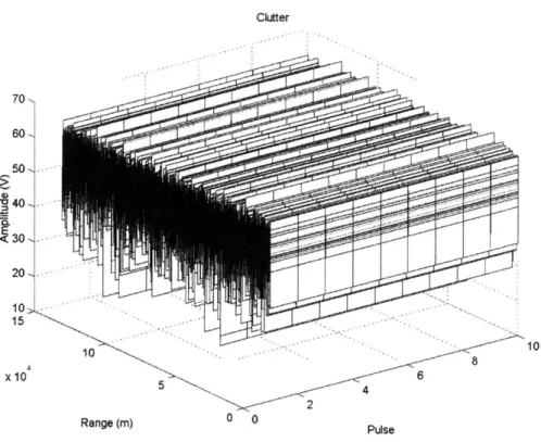
2.3.3 Jamming Model

Jamming, or ECM, is the area of electronic warfare designed to exploit and prevent the effective use of friendly radar systems. Passive jamming techniques such as chaff have little motion and are thus ineffective against PD and MTI radars. Active jamming techniques are of greater concern for PD/MTI radars and can be divided into noise jamming and deceptive electronic countermeasures (DECM).

Noise jamming is similar to raising the level of thermal noise. It attempts to interfere with the normal operation of a radar by transmitting enough power in the frequency spec-trum of the receiver to raise the noise floor above the strength of any target signals [10]. This can be simulated by increasing the noise level within a CPI.

Deceptive jamming techniques attempt to deceive a radar by repeating back its trans-mitted signal to mislead the receiver. These techniques may be used to create false targets, disrupt tracking, and report false positions [10]. For a radar using binary phase-modulated

Clutter 70 60 50 S30- 20_-15 10 8 x 10 6 2 Range (m) 0 0 Pulse

Figure 2-8: Clutter Component

waveforms, a repeater as shown in Figure 2-9, is required to capture the transmitted code

to successfully create a false target

[141.

previous pulse to create 15 false targets. The resulting data is shown in Figure 2-10. Notice that there is no jamming signal in the first PRI due to the implementation of this type of repeat-back jamming.

Trigger

Delay Memory _Receiver

Antennas Variable

Delay

Stored

Amplifier]

Control

Pulse

Figure 2-9: Repeat-Back Jammer Block Diagram

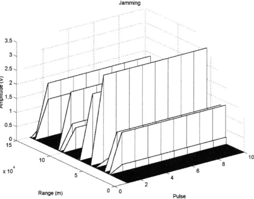
When the repeater successfully captures a radar's transmitted waveform, it can create targets at the receiver input and jamming the radar becomes trivial. The effect of successful

Jamming 3.5- 3- 2.5-15 10 810 X 10 5 _{4 6} 2 Range (m) _{0 0 Pulse}

Figure 2-10: False Targets Created by Repeat-Back Jamming

jamming on an MTI radar is shown in Figure 2-11 where only one of the many targets is real. The variable pulse-code radar addresses this vulnerability by mitigating the effectiveness of the repeated signal. This will be further explored in Chapter 6.

MTI Filtered Return 80 60 40, M20, -20 --156 x 10 ₅ 4 2 Range (m) _{0 0 Doppler}

Figure 2-11: MTI Filtered Return with Repeat-Back Jamming

2.4

Return Processing Model

Radar systems employ many signal detection strategies to distinguish between desired echoes and interference. Passive and active filtering techniques at the receiver are used to increase signal-to-noise and signal-to-clutter ratios.

The composite return consisting of the targets and environmental factors are first sam-pled and filtered using either matched filter or pulse compression filter techniques. An adaptive digital equalization filter may be added when using variable pulse-codes. The fil-tered data is then Doppler or MTI processed. The simulation allows the user selection of sampling rate, receiver filter type, pulse compression filter length, windowing, MTI imple-mentation, and equalization filtering as shown in Figure 2-12.

2.4.1 Pulse Compression

Pulse compression (PC) and matched filtering (MF) are signal processing strategies for signal detection improving range resolution and SNR when using waveforms such as binary phase encoded PN codes. These strategies simultaneously achieve the high output energy of a long transmit pulse and the range resolution of a short pulse.

Figure 2-12: Return Processing Variables

The pulse compression filter is designed to produce a flat frequency response at its output given the signal for which it was designed at its input [1]. Thus, the frequency response of the pulse compression filter is the reciprocal of the input signal frequency spectrum. Let the frequency response of the pulse-code sequence in question, s(n), be given by:

S(f) = DFT(s(n))

where DFT represents the discrete Fourier transform. Then, the pulse compression filter's frequency response is given by:

1

H(f) = (2.6)

SMf)

When multiplied with the input frequency spectrum S(f), the time response of the resulting flat output spectrum would therefore approximate a dirac delta function, thus minimizing signal sidelobes:

Y(f) =S(f)H(f),

S(f), = 1,

= 1 < OOt)

y(t) = (t) (2.7) 2.4.2 Matched Filtering

Pulse compression and matched filtering are similar and the terms are often mistakenly used interchangeably. Their difference is an important distinction in this thesis. Whereas the pulse compression filter is designed for a flat output spectrum, the matched filter design criteria is to achieve a maximum signal-to-noise ratio. This criteria is met when the matched filter is the time reversed input signal [1],

h(t) = s(tm - t). (2.8)

Thus, its frequency response is the complex conjugate of the Fourier transform of the input signal multiplied by a time shift factor:

H(f) = S*(f)ew't, (2.9)

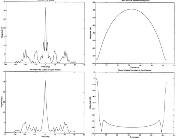
where tm corresponds to the pulse width of the transmitted signal. A comparison of the time and frequency responses of a matched filter and pulse compression filter given a 32-bit PN-code as the input sequence are compared in Figure 2-13. The first two plots show the magnitude and frequency response of input code sequence. Notice below in the next row the formation of the matched filter as the time reversed input, and the formation of the pulse-compression filter as the reciprocal spectrum. The last four plots compare the output of the matched filter with the pulse compression filter. Notice the flat frequency-spectrum of the pulse compression filter output and the flat sidelobes in its time response. This property will become significant in Chapter 4.

2.4.3 Weighting

Weighting, or windowing, is a technique used to reduce sidelobe levels at the expense of broadening the main-lobe width and a slight reduction in SNR [7]. Sidelobe levels of the matched filter output will become a problem for the variable pulse-code radar system and weighting will be explored as a solution.

Frequency Specotur 0.5 --- 15 - 0--0.5 - _o. -1. -0 5 10 15 25 35 0 0 20

Tinm (step) Frequency

Matched Filter Ttme Flesponse Pulse Compresson Filter Frequency Spectrum

5 0.5-

-10-0I

Time (step) Frequency

Matched Fifter Output Pulse Compression Filter Output

30- 30-25- 25-20 20, 15 ' - 15-10 1. 5- -5-0- .4w 0. 5 5 -30 -20 -10 _{Tme (slop)} 0 10 20 30 -30 -20 -10 0 10 20 30 Tme (step)

Matched Filler Oulput Frequeny Spectrsmi Pulse Compression Filter Output Specrumn

40 35 -- ₃₅ -30- _30. 2 25 5 20 -20-15- 15-0 10 20 30 40 50 00 l1o 0 to 20 30 40 50 0 Freqency Frequency 32-81 P- Cods I AA/Lf~

A(\ /"\h

f~/'\

1

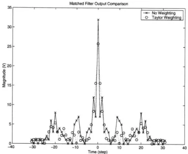
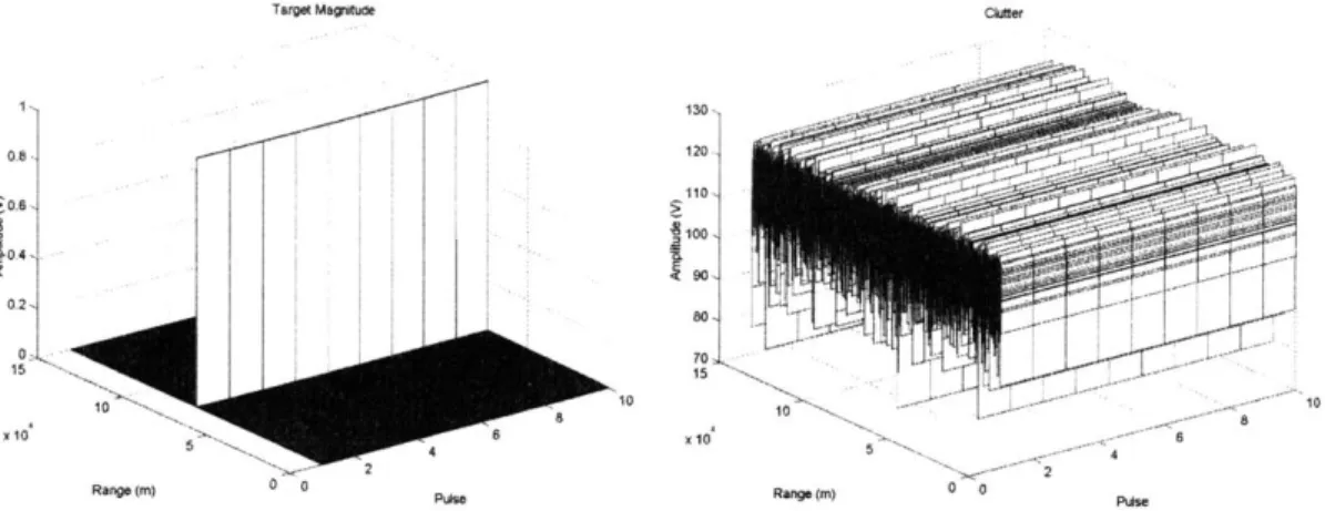
This is the case when weighting is applied across PRIs in a CPI to shape the Doppler spectrum. Weighting may also be applied in the frequency domain to reduce sidelobes in the time domain and shape the waveform of the filtered pulse. Both techniques are implemented by the simulation. The user is able to choose from uniform (none), Hamming, Hanning, Chebyshev, Taylor, and Dolph-Chebyshev weighting functions.

Figure 2-14 shows the application of a 63-point Taylor window on the matched filter output. The window is applied in the frequency domain to reduce sidelobe levels in the time domain. The result is shown in Figure 2-15. Notice the reduction in sidelobe levels at the expense of a lower peak value and broadening of the main lobe. The first sidelobe peak after the apparent null of the weighted output shows a 1.2 dB improvement.

Matthed Filter Oulput _{Taylor Window Apped m Frequ-ncy}

30-. :20 - 105 --40 -30 -20 -10 0 10 20 30 T,, (Stp) Malthed FAKe Output wraylor Westaow

-40 -30 -20 -10 0 10 20 30

Ti-. (step

Figure 2-14: Matched Filter

020 - -30- -70--W0 0 10 20 3 0 5 0 70 Teie (step)

Output with Taylor Weighting

2.4.4

Doppler Processing

Doppler processing separates signals with different range rates within the radar return. This allows us to separate the relatively stationary clutter from moving targets. The motion

30

-1-35

55

-10 20 30 40 50 60 70

Freqaoncy Taylor WMM arform M mTo1 0111102

40

Matched Filter Output Comparison -+-No Weighting 0 Taylor Weighting 30-25 5 20 S15- 10- 5-C0 -40 -30 -20 -10 0 10 20 30 40 Time (step)

Figure 2-15: Matched Filter Output Weighting Comparison

contributes a frequency shift to the reflection in proportion to its velocity. By comparing the received signals coherently across several pulses, the frequency shift and therefore range rate, can be observed. The relation between target velocity and Doppler frequency shift is shown in Equation 2.1.

The amount of target gain due to Doppler processing can be calculated. Suppose we have a noisy input signal,

x(n) = e2" + v(n).

The discrete Fourier transform (DFT) is then performed to Doppler process the signal. The result is

2wrkn X(k) =

x(n)e

X(k) = ei(a- " + v(n)e--2 .

n

The power of this signal is defined by

P(k) = E{x(k)x*(k)}

=

Z

+

+

If we assume Gaussian white noise, we can ignore the cross terms since the noise has zero

mean. In addition, the noise is uncorrelated from sample-to-sample and from pulse-to-pulse. Therefore, the expected value is nonzero only for n = m. Our equation may now be simplified to

P(k) = eNa N Y )(-") +

S

n,m n,m

If = 27, then for the first term,

eAa-)(n-m) = N2, _(2.11)

n,rna 2-rk

which is the peak energy of the target signal after Doppler processing. For the second term,

5

- m)e-i("- 2jO = Na2_,

(2.12)

n,m n

which is noise energy level after Doppler processing. From Equation 2.11 and Equation 2.12, we can calculate the Signal-to-Noise (SNR) ratio,

N

_N

SNR ~ N2 - N -N-SNRO.

Na2 U2

Therefore, the Doppler processing gain is 10

logio(N)

the CPI. For 10 samples, the Doppler processing gain is 10dB.

The advantage of Doppler processing is the ability to detect targets buried within a significantly stronger clutter return, as long as there is a difference in velocity. This case is taken to the extreme in Figure 2-16 where we see the clutter dominating the target signal by approximately 100 dB. Figure 2-17 shows the return after Doppler processing. The clutter energy has been transformed into the zero Doppler bin and the target can now be clearly seen in the last Doppler bin.

2.4.5 MTI Implementation

Moving Target Indication (MTI) radar uses the same physical phenomenon as pulsed Doppler radar. Doppler frequency shifts over multiple pulses are used to separate sig-nals by velocity. MTI adds the additional objective of removing clutter to improve the

Target Magrntude 130 120 110,-100 x 1001 X10 S2 Rn () 0 0 PUSS

Figure 2-16: Target and Clutter Comparison for Doppler Processing

Doppler Processed Retum

200 150 -100 -4) V 50 0-1 -50 15 X10 Range (m) Doppler

Figure 2-17: Doppler Processed Radar Return

1 _ 0.8-0.6 04. 0.2, 1 x15 100 Range (m) 0 0 Pulse Ckuter g -10 5 0 0 246 8 10

signal-to-clutter ratio [11]. Early MTI systems use delay-line cancellers and were limited in complexity by the capability of analog acoustic devices. The availability of digital tech-nologies has significantly enhanced MTI processing.

The implementation of MTI used in this thesis applies a three-point digital low-pass filter to the Doppler frequency spectrum. This filter, whose time samples and frequency response is shown in Figure 2-18, attenuates all low frequency signals including clutter and leaves only detected targets. The result after MTI processing is shown in Figure 2-19.

UTI FilEW IM R eSp M . MTI Filter Frnquency Responm

3 ₂₀ 2- 10-1 ₀ -2- -10 -2- -20-r -2 L I

1

Figure 2-18: MTI Filter Impulse and Frequency Response

2.4.6 _{Adaptive Digital Equalization Filtering}

When using a variable pulse-code radar, the output of the Doppler filter will be degraded beyond use due to the differences between codes. This is fully explored in Chapter 3. An adaptive digital equalization filter is applied to the matched filter output as one approach to recover this performance. This type of filter attempts to equalize an input to a given function. It will change its coefficients to minimize the error between the input sequence and that function.

For this thesis, the implementation of the equalization filter will be performed digitally in the frequency domain. The details of the process and results are discussed in Chapter 5.

MTI Filtered Return 60 40 S20 0 -20 -40 -> 15-A8 10 7 X 10 55 3 2 Range (m) ₀ J Doppler

Figure 2-19: MTI Processed Radar Return

2.5

Simulation Output

The individual elements in the formation of the simulated radar return may all be plotted along with the intermediate and final results of any return processing. The user is able to plot the target, noise, clutter, jamming, composite return, filtered return, weighted return, Doppler processed return, MTI processed return, and adaptively equalized returns as shown in Figure 2-20.

Plotting Options

Noised MTI E qualze /T

Chapter 3

Variable Pulse Code Radar

The variable pulse-code radar modifies the transmitted waveform of the pulsed Doppler or MTI radar. Instead of selecting one PN code sequence, the variable pulse-code radar transmits a newly selected code with every PRI as shown in Figure 3-1. The transmitted waveform is then no longer predictable and thus difficult to jam.

Ccnstant 32-4it Pulse-Cods, 10 Pulse CPI Varable 32-bit Pulse-Code, 10 Pulse CP

30

10--0 -P 8

-0 4

Tim (stop) _{0 0 PRI}

1.5,-_1 30 ₁₀ 206 10 4 Tre0 0Pl Figure 3-1: Constant and Variable Pulse-Code Comparison

3.1

Doppler Degradation

The use of variable pulse-codes presents several problems. The matched filter output from the radar echoes of each pulse will have different range sidelobes. When the return is Doppler processed, the effect of changing sidelobe magnitude and phase results in a spreading effect thereby creating false signals in the Doppler spectrum. Over multiple clutter points, this effect significantly degrades the signal-to-clutter ratio.

For example, let us examine the Doppler spectrum of the matched filter output given a point scatterer. When the same pulse-code is used for each PRI, the matched filter output in that range bin will be constant and contribute to only one Doppler bin in the Doppler spectrum as we see in Figure 3-2.

Matched Filter Output with a Constant Pulse-Code Doppler Spectrumr (Constant Code)

25,s5, .--- 60 --. 10 400 Ran08 (M) 0 0 350 . 300, 250 . 200 , --50 - .. -. -50 -100 - -- -60 10 40 6 0 0

Plse Repetition Interval

~Doppler

Figure 3-2: Matched Filter Output and Doppler Spectrum for a Constant Pulse-Code However, when a different pulse-code is used for each PRI, the sidelobes of the matched filter outputs will differ due to the variations between pulse-codes. These variations will proportionally contribute to different Doppler bins. The Doppler spectrum of the outputs will be spread across all Doppler bins. For this paper this will be referred to as a false Doppler effect since it appears that the energy is in the wrong Doppler bin. We see this spreading in Figure 3-3.

Matched Filter Output wilh Variable Puise-Codes Doppler Spectrui (Vanable Codes)

40, 350 . 3- 250-10-20 -00--20 -80 50 80 10 010

Ranga (M) 0 0 u R Inl Range (M) 0 0 Doppler Frequency

3.1.1 Target Effects

Fortunately, the peak value of the pulse-compressed target return signal is minimally af-fected by changing from constant to variable pulse-codes. In the absence of clutter, the false Doppler effect created by varying sidelobes is insignificant for the relatively low number of individual targets. Given that the length of every different pulse-code remains the same, the magnitude and phase of the zero-lag matched filter output will remain the same and thus the return signal can be successfully Doppler processed.

This is proven by calculating the variance of the matched filter output at zero-lag given

a point scatterer. In the absence of noise and clutter, the return signal is r(n) = s(n - m),

where s(n) is a randomly selected, 32-bit PN code and m denotes some time delay. At

m = _{0, given a sampled signal, we can define the matched filter output as}

min(N,N-1) y(n) = E s(n - k)s(N - 1 - k), or, k=max(,n-(N-1)) min(N-1,N-1+1) = E s(N - 1 + l - k)s(N - 1 - k), (3.1) k=max(0,l)

where 1 =

n

>

peak output is at (0) = y(N - 1) and the first sidelobes' value is at (1) = y(N). From

this, we can compute the matched filter's range sidelobe performance. In order to perform

this analysis, we will model Sn, a randomly chosen 32-bit code sequence, as a stochastic

process [8]. _{This allows computation of the mean of the matched filter output's range}

sidelobes.

To simplify analysis, let S,, s(N - 1 - n), where N is the number of samples. The

elements, Sn, belong to the set S =

{-1, +1}

Furthermore, Si is assumed orthogonal to Sj for all i 54

j.

autocorrelation of Sn is

R(k+l,k) = E{Sk+jSk},

= _{; =0}

(3.2)

0 ;

4i0

Returning to equation 3.1 and substituting Sk for s(N - 1

(l)

min(N-1,N-1+1)

E Sk+lSk,

k=max(0,1)

from which the mean value of the sidelobe level quickly follows via Equation 3.2

min(N-1,N-1+l) =

Y

E(

where N is the number of samples of S,.

To calculate the variance of p(l), we must first compute the second moment of

y(l);

E{y2_{(l)}= IEE{Si+,SiSj+Sj}, or}

i= j

= Y:EfSi2±si~+ EES+iSi}ESISjjl

i=j

For the peak, zero-lag value where 1 = 0,

E{ 2(0)} = E{S4} i=j + E E{sf }E{Sh}, i#j Efy2(0)} = N + N(N - 1) = N2 . (3.6)

For the sidelobe, non-zero-lag values where 1

$

N -

l|

E= E{Sf S+ ₁} +0, or

i=j

= N - l. (3.7)

Let us define N = N - 1l. Then from Equation 3.6 and Equation 3.7, we find that the

second moment is (3.3) E{Q(l)} i#j (3.5) or, k) yields

E 2(1) = , (3.8)

N ; ?if0

where N is the number of terms in the overlapped region and equal to N -

111.

Equation 3.4 and Equation 3.8, we see that the variance of the matched filter's range

sidelobes,

y(l),

Var{y(l)} ={ ' (3.9)

>-111

1=4

Thus, given any PN code sequence, the peak (zero-lag) value of the matched filter output has no intrinsic variation with code, but the non-zero-lag values have a non-zero variance. The implication is that given a set of random sequences of length N, the peak values of the matched filter output will produce an accurate Doppler frequency estimate. However, the Doppler spectrum from the sidelobe non-zero-lag values will not be resolved due to the variations from pulse to pulse.

This result is also verified by simulation. The match filtered target return in the absence of clutter shows a constant peak value but different sidelobes. A plot of the Doppler processed return from a variable pulse-code radar in the absence of clutter is shown in Figure 3-4.

3.1.2 Clutter Effects

When clutter is reintroduced, it acts as multiple point scatterers, each with varying sidelobes as we saw in Equation 3.9. This variance gives each sidelobe a potentially non-zero value in the target's range bin and final Doppler spectrum. The aggregate spreading effect of these false Doppler values created by the range sidelobe leakage of clutter thus effectively buries the target signal. This can be seen in Figure 3-5.

To quantify this effect, we need to look at the Doppler spectrum. Let x, (t) represent

the target in MF gate 1. The Fourier transform of the 11h gate is

P-1

Yi(w) = l ip(O~xi(Ae -jwp. (3.10)

p=o

where

yp(l),

Doppler Processed Return 60-50 --7 Target 40 30- 20-.0 0 10 -4 --10 - -30-x151 5 4 Range (m) _{0 0 Doppler}

Figure 3-4: Variable Pulse-Code Radar Doppler Return without Clutter

Doppler Processed Return

110 Cut 100 90-50 40 30 15-o 70 x 101 Range (m) _{0 0 Doppler}

P-1

E{Yo(w)} = E E{pp(O)}xo(p)e-iwP p=o

Substituting with Equation 3.4,

P-1 E{Yo(w)} = N E xo(p)ei-P. p=o E{1Yo(w)j2}

Z

Z

5

Combining Equation 3.12 and Equation 3.13 we see that the variance is

Var{Yo(w)} = 0;

(3.12)

(3.13)

(3.14)

17 0.

This is as we expected; using variable pulse-codes will not affect the peak value of the MF

output. For the 1 / 0 case the mean, second moment and variance are

E{Y(w)} = P-1 E{yp(l)}x(p)e-iwP, p=o 1 = 0. (3.15) (3.11)

E{IYi(w)12_}

=

ZE{Qp(l)pq(l)}x(p)x*(q)e-jw(P~q)

p,q

= (N

p=q

- j1j)xi(p)x*(q)e-jw(P-q) + E E{Qip(l) }E{yq(l)} 1(p)X* (q)e~-w(P-q)

ppq

P-1

E{IYi(w) 12}

=

111)

E

p=o

P-1

Var{YijLl} = (N -

Ill)

Z

p=O

(3.16)

(3.17)

Thus, the variation in range sidelobe levels causes a rise in Doppler filtered output sidelobes.

Now suppose that in MF bin 1 = 0 we have

X0(p) = xt(p) + xc(P). (3.18)

where xO is our output composed of a target, xt, and clutter, x,. For analysis, we can assume

that the target and clutter Doppler are easily separated. Substitution in Equation 3.11 yields

P-1

o(L,) = N E (xt (p) + xc(p))e-'P p=O

(3.19)

where P is the number of pulses in the CPI. If we let Xt = -tejwP, the Doppler spectrum

becomes

Y0(w) = N E atej('t-w)P + N E Zxc(p)e-jP, P

(3.20)

P

Now we can compute the final signal-to-clutter ratio. With wt = w, from Equation 3.20, we

see that the target signal energy, Et is,

Et = (NPat)2.

The clutter signal energy, Ec, is computed by

Ec = N 2 E{xc(p)x*(q)}ejw(P-q)

P~q

We assume xc(p) and xc(q) are independent. For all p 5 q, the expected value of xc(p) and xc(q) is zero for a Gaussian distribution. Thus, in the remaining case where p = q, the energy is

Ec = N2 Z E{xc(p) 12} P

Using Parseval's theorem and Raleigh's energy theorem which equates energy in the time domain with energy in the frequency domain, we calculate the clutter signal energy as

Ec = BcN2_No,

(3.22)

where Be is the bandwidth of the clutter and No is the spectral level of the clutter. From Equation 3.21 and Equation 3.22, the computed signal-to-clutter ratio is

(put)2 _(3.23)

BcNO

To compute the effect of the clutter sidelobes on the target signal, suppose we have

some type of clutter signal present in the previous range bin. The 1 = 1 correlation lag of

this clutter signal will affect the 1 = 0 correlation lag of the target signal. It will cause an

increase in spectral power as per Equation 3.17.

P-1

Var{Yjwj} = (N - 1l) E E{|xi(p)j2

}.

p=0

Using Parseval's theorem this becomes

Var{Yj(w)} = (N - 1lI)NoBc. (3.24)

Summing over all non-zero-lag values, 1, the total contribution to clutter from these cells

becomes

N-1

Z Var{Y(w)} = NoBc2 Z(N-l)

I =1

Thus,

Var{Y(w)} = NoBc(N - 1)N. (3.25)

Let us compare this to the non-overlapping sidelobe Doppler spectrum that we calculated in Equation 3.23. When we introduce random MF range sidelobes, we see that our noise power level has increased by a N(N-1) factor that is not separable from the target.

(Pa-t)

This leads to approximately a N2

reduction in SNR. For a 32-bit PN code where N = 32,

this is approximately a -30dB (1Olog32x31) loss in SNR performance. Figures 3-6 and 3-7

rotate our three-dimensional plots to show the profile of the Doppler spectrum for a pulsed Doppler radar using constant versus variable pulse-codes. We see that there is in fact a

30dB clutter sidelobe ceiling over the target in the Doppler spectrum due to the MF in a

variable pulse-code radar.

This empirically verifies the calculated performance degradation associated with matched filtering in a variable pulse-code radar. We have proven that zero-lag peak values have no variance when matched filtered. However, the variance in clutter sidelobe strength across all non-zero-lag values create a false Doppler signal. This results in a significant SNR loss and buries the target in the Doppler spectrum. Thus, any attempt to recover this performance will need to address the strength of these clutter sidelobes. This can be done directly, which

Constant Pulse-Code Radar Doppler Return Profile 120 r Cluttr-> -. ...- ' * * '- * ---.. ... 4 5 6 7 8 9 10 Doppler

Figure 3-6: Constant Pulse-Code Radar Doppler Return Profile

Variable Pulse-Code Radar Doppler Processed Profile

Clutte r--/ --x

..

..

...

.. N.

Figure 3-7: Variable Pulse-Code Radar Doppler Return Profile

Target-- -- -.-.-. .. 100 F --. 80k-4) 60 - - .- .- .-. Range (Tm) 40 - - . 20~77 / 01

I,

...

Chapter 4

Pulse Compression Filtering

In the previous chapter, we discovered that for a variable pulse-code radar, Doppler and MTI processing performance is significantly degraded by clutter sidelobe strength at the matched filter output. Using a different pulse-code for each PRI results in a different matched filter for each PRI. When the clutter component of the radar return is matched filtered, the output response is different for each PRI. Though the zero-lag peak values remain unchanged, the sidelobe values differ significantly. These differences spread energy across the Doppler spectrum. Over many clutter points, the aggregate effect is a loss of the target signal-to-clutter ratio.

To mitigate this Doppler spread effect caused by using variable pulse-codes, we can either reduce clutter sidelobe strength at the matched filter output or process the return signal to undo the negative effects of variable pulse-codes. Performance recovery using digital signal processing techniques will be discussed in the following chapter.

4.1

Matched Filter Waveforms

Clutter sidelobe strength at the matched filter output is dependent on the variance of the non-zero-lag values of the transmitted waveform's autocorrelation function as we saw in Equation 3.9. Its contribution to the Doppler spectrum is shown in Equation 3.17. Thus, the magnitude of the Doppler effect is dependent on the transmitted waveform which is determined by the selected pulse-code sequence. By selecting code sequences with minimal non-zero-lag variance, we can attempt to mitigate the false Doppler spread effect.

4.1.1

Sidelobe Reduction

The study of code sequences and their properties is a significant field of study in digital communications and signal processing. To recover Doppler performance, our code selection will focus on minimizing the output sidelobes of the matched filter. Barker codes are a

small family of codes, none longer than length N = 13

[3].

R, )0 N T (4.1)

±1,0, r 0

where Rc(T) is the autocorrelation value at lag T. Notice that all sidelobe values are within

±1. This is a desirable property given our requirements, but these codes are unsuitable for

the application at hand. With a maximum length of 13-bits and such a small set of codes with this ±1 sidelobe property, the waveforms from a radar using Barker codes would be

highly predictable and susceptible to jamming.

For the 32-bit codes used in this simulation, we can apply the same selection concept

by relaxing the criteria posed in Equation 4.1. A search through all 32-bit codes yielded no

codes for whom all sidelobe values are within ±2. However if we allow

Re(T) =NIT = 0 .(4.2)

±3,±2,i1,0, T 0.2 ₄

then there are 3,376 codes to choose from. Figure 4-1 shows the Doppler spectrum profile when using randomly generated pulse-codes and Figure 4-2 shows the Doppler spectrum when using our set of ±3 codes. The comparison shows approximately a 7 dB drop in the clutter floor when using the ±3 codes.

Let us return to our variance calculation in Section 3.1.2 to verify our theory against the empirical results. As in Section 3.1.1, we treat the codes as a stochastic process. Equation 3.9 gives us the variance of the non-zero-lag values of the matched filter output. Figure 4-3 shows the results of an exact analysis [4] of the variance of the 32 bit PN sequences' auto-correlation lags, i.e., range-sidelobes for both the unfiltered case and the case where the 32 bit sequences were filtered to include only those sequences for which the range-sidelobes were within a ±3 bin range. The mean of these range-sidelobes is zero. The average of the variance over non-zero-lag values of the unfiltered sequences is 16.5

Doppler Processed Return using Random Pulse-Codes Range --...-...-. Clutter -/

/

Figure 4-1: Variable Pulse-Code Radar Doppler Return using Random Codes

Doppler Processed Return -+/-3 MF Sidelobe Codes 110 r 105 F - - - -Range

/

Clutter-- >

1

Figure 4-2: Variable Pulse-Code Radar Doppler Return using ±3 Codes

110 r-105 -100 - --95 F -a 4) 90 85 80 75 70

100

ru

-using Equation 3.9. The variance for the censored data is seen to alternate between 4.75 and 2.6 with an average over the non-zero-lag values of 3.43. This is close to a variance of 3.0 which would be arrived at by assuming uniform distribution of the non-zero-lag value

range-sidelobes between ±3. Based on the exact analysis, there is a 10log( 6) = 6.8219

dB improvement which matches the empirical result. Although 6.8 dB is a significant improvement, it is not nearly enough to even begin to recover the target SNR.

Sidelobe Variance versus Lag

35

Var Uncensored

....

...

V

a r + /- 3

~

x

10

0

5

10

15

20

25

30

Lag Value

Figure 4-3: Mean and Variance of Random and ±3 32-bit PN Codes

4.2

Pulse Compression Waveforms

We have verified that selecting codes with a limited matched filter output sidelobe

level

improves our SNR. Lower sidelobe

levels

lower

less

function as N -+ _{inf. Again, using Equation 3.9 and Equation 3.17, we see that if there is}

zero variance in the non-zero-lag values of the ME output, then there is zero contribution to the Doppler spectrum.