An Analysis of Engine Assembly and Component Production Behavior
by
Thomas B. Blake
B.S. Mechanical Engineering, United States Military Academy, 1991
Submitted to the Sloan School of Management and the Department of Mechanical Engineering in Partial Fulfillment
of the Requirements for the Degrees of
4~ste~ u£ Sc:ience in Management I"/t, ; 1-and
Master of Science in Mechanical Engineering
In Conjunction with the Leaders for Manufacturing Program at the
Massachusetts Institute of Technology
May 1999
( 1999 Massachusetts Institute of Technology. All rights reserved.
Signature of Author
Sloan School of Management
Department of Mechanical Engineering
May 7, 1999
Certified by
Nelson Repenning, Assistant Professor of Management
~..
Sloan School of Management-,
T...
hesis Supervisor,
F Daid E. c T~r-fs o
of
David E. Hardt,roessor of Engineering
Department of Mechanical Engineering
flils S1derv'nr
Accepted by
Lawrence S. Abeln Director of Masters Program
Sloan Scb "El.anagement
Accepted by
_4m~Gi~l·-
~
i ArA
. Sonin
Chairman of the Graduate Committee
Department of Mechanical Engineering
Certified by i ·-···-·· ·t, ·i 1 -···
1041"ra
An Analysis of Engine Assembly and Component Production Behavior
by
Thomas B. Blake
Submitted to the Sloan School of Management and the Department of Mechanical Engineering in partial fulfillment of
the requirements for the degrees of
Master of Science in Management
and
Master of Science in Mechanical Engineering
ABSTRACT
This study analyses the information and material flow through a component manufacturing and
turbine engine assembly system. The intent of this work was to understand the inefficiencies associated with
the current system, and to propose solutions which would prove valuable to the entire value chain, not only to one manufacturing site. This work was accomplished by identifying a significant problem in the system, developing a model to replicate historical behavior, then developing solutions to improve material and information flow.
The shipment rate of engines from the assembly facility was found to follow a "hockey stick" pattern throughout each production quarter (a three-month cycle), meaning that shipments increased exponentially toward the end of each quarter. Shipments were traced back through the component manufacturing facilities,
and the exponential increase of component shipments was shown to follow that of assembly shipments.
Interviews were primarily used to establish critical variables in the system, and a system dynamics modeling
technique was used to generate a model that mirrored historical shipment data. The model was then manipulated to test the sensitivity of specific production variables, and suggestions were made to improve
material and information flow.
Finally, a component kit plan was developed that added value to the assembly facility by delivering gear products by order number rather than as separate components. Also, the component production facilities
benefit by shortening the existing information feedback loop between component manufacturing and assembly and allowing more level production with less variability amplification from the bullwhip effect. Demand Flow
Technology is introduced as a means to then affect the entire supply chain, including supporting functions not directly related to manufacturing.
Thesis Advisors:
Assistant Professor Nelson Repenning, Sloan School of Management
Acknowledgements
The author gratefully acknowledges the support and resources made available through the Leaders for
Manufacturing Program, a partnership between MIT and major U.S. manufacturing companies.
A personal note of thanks to Nelson Repenning, David Hardt and Hans Laudon for their guidance.
Table of Contents
ACKNOWLEDGEMENTS ...
...
...
5...
TABLE OF CONTENTS ...
7
TABLE OF FIGURES ...
9
CHAPTER 1 INTRODUCTION ...
...
10
1.1 PROBLEM MOTIVATION ... 11 1.2 INTRODUCTION ... 12CHAPTER 2 MODEL BUILDING ...
15
2.1 MODEL INTRODUCTION ... 15
2.2 A MANUFACTURING MODEL ... 17
2.3 INDUSTRIAL DYNAMICS ... 18
2.4 COMPONENT PRODUCTION AND ENGINE ASSEMBLY ... 24
CHAPTER 3 MANUFACTURING MODEL DEVELOPMENT ... 26
3.1 ANALYSIS OF INTERVIEWS AND DATA ... 26
3.2 CAUSAL LOOP DEVELOPMENT ... 29
3.3 MODEL DEVELOPM ENT ...42
3.4 RESULTS ... 48
3.5 RECOMM ENDATION ... 54
CHAPTER 4 KIT PLAN ...
56
4.1 KIT PLAN INTRODUCTION ... 56
4.2 KITrING DEVELOPMENT ... 57
4.3 PROS AND CONS . ... ...61
4.4 W HAT TO IIT?... 64
CHAPTER 5 INTEGRATING PRODUCT OWNERSHIP ... 70
5.1 BACKGROUND ... 70 5.2 A PPLICATION ... 72CHAPTER 6 CONCLUSION ...
...
75
6.1 INTEGRATION ... 75 6.2 FUTURE WORK ... 77REFERENCES ...
79
APPENDIX A ...
80
MANUFACTURING MODEL DOCUMENTATION ... 80
APPENDIX B ...
105
MANUFACTURING MODEL ... 105
Table of Figures
FIGURE 2.1-1 FIGURE 2.1-2 FIGURE 2.1-3 FIGURE 2.3-1 FIGURE 2.3-2 FIGURE 2.3-3 FIGURE 2.3-4 FIGURE 2.3-5 FIGURE 2.4-1 FIGURE 3.2-1 FIGURE 3.2-2 FIGURE 3.2-3 FIGURE 3.2-4 FIGURE 3.2-5 FIGURE 3.2-6 FIGURE 3.2-7 FIGURE 3.2-8BIRTH RATE LOOP... ... 15
DEATH RATE L ...OOP 16 COMBINED BIRTH-DEATH LOOPS ... 16
DISTRIBUTION MODEL STRUCTURE ... 19
STEP ORDER INPUT ...21
SINE ORDER INPUT ... 22
STEP INPUT (MATERIAL FLOW) ...23
SINE INPUT (MATERIAL FLOW) ... ...23
STRUCTURE SIMILARITY...25
QUARTERLY
ENGINE
SHIPME N T S
. ...
29
QUARTERLY GEAR SHIPMENTS TO STORES ... 30
N)RMALIZED QUARTERLY GEAR SHIPMENTS ... 31
AVERAGE GEARS/WEEK ... 32
PRODUCTION/ASSEMBLY BALANCING LOOPS . ... 33
ORIGINAL COMPLETION REFERENCE MODE ... 34
REVISED COMPLETION REFERENCE MODE ... 34
BALANCING ASSEMBLY LOOP ... ... 37
FIGURE 3.2-9 ASSEMBLY WIP REINFORCING LOOP ... ... 38
FIGURE 3.2-10 COMPONENT EXPEDITING BALANCING LOOP ... 39
FIGURE 3.2-11 ENGINE EXPEDITING BALANCING LOOP ... ... 40
FIGURE 3.2-12 C)MPLETE CAUSAL LOOP STRUCTURE ... ... 41
FIGURE 3.3-1 UNFILLED GEAR ORDERS ... 43
FIGURE 3.3-2 GEAR W IP ... 43
FIGURE 3.3-3 MODEL PRODUCTION/ASSEMBLY DELAY ... ... 45
FIGURE 3.3-4 THEORETICAL PRODUCTION/ASSEMBLY DELAY ... 45
FIGURE 3.4-1 WIP BASE CASE MODEL RESULTS ... 49
FIGURE 3.4-2 WIP ADJUSTMENT RESULTS ... 51
FIGURE 3.4-3 STOCKOUT DELAY RESULTS ... 52
FIGURE 4.2-1 PRODUCTION-ASSEMBLY PROCESS FLOW ... 58
FIGURE 4.2-2 WAREHOUSE OVERHEAD VIEW ... 60
FIGURE 4.2-3 ENGINE RACK AND PART TRAY . ... ... 61
FIGURE 4.4-1 REPRESENTATIVE KIT ... 66
FIGURE 4.5-1 EXISTING SYSTEM WITHOUT IKITTING...68
Chapter 1 Introduction
"An information-feedback system exists whenever the
environment leads to a decision that results in action which
affects the environment and thereby influences future decisions."
-Jay W. Forrester
1.1 Problem Motivation
This project began as a local optimization of a gear production facility manufacturing process within the framework of a larger engine assembly facility with multiple component production centers and a central assembly center. It was determined that a local
optimization would contribute to certain operational improvements within the gear center,
and could have some effect on upstream and downstream activities, but the improvements would remain limited in effectiveness due to the gear center's integration with a final engine
assembly schedule. Therefore, the scope of the problem was broadened to incorporate the
entire supply chain, from procurement of raw materials and externally manufactured
components through assembly and delivery to the customer. The specific issues centered on component production and engine assembly rates (contributing directly to delivery
performance), and inventory levels throughout the chain. Delays in information and material flow between component centers led to a bullwhip effect, which amplified
production schedule disruption and inventory levels, and severely limited the gear facility's ability to smooth production rates and maintain delivery performance without continuous expediting. The problem presented in this work involves a specific manufacturing
environment, but has been developed generically to apply to many manufacturing situations which manufacture and procure components, and assembly those components into final products according to a forecasted schedule.
1.2 Introduction
The turbine engine facility represented by this study designs and manufactures auxiliary power units (for commercial and regional airlines, and business/military aircraft) and turbofan, turboshaft and turboprop propulsion engines (for business aviation, regional airlines, military aircraft and marine and industrial markets). Turbofan engines support applications in the 3500-5000 lb. thrust range in business aviation and 7000 lb. thrust range in regional jet applications. Auxiliary power units support applications from corporate jet through the commercial airliner range. Also, the company provides maintenance service and repair parts through a worldwide service and support network.
At the engine facility, a main assembly facility receives both purchased and internally manufactured parts, and maintains sole responsibility for engine assembly and shipment, and
kit and spare part order consolidation and shipment. Aside from externally purchased parts,
three component manufacturing centers on the campus support the assembly facility with manufactured parts and subassemblies. Manufactured products from these three facilities include gears and shafts, subassembly housings and machined casings, compressor and turbine rotating groups, and a variety of static sheet metal components.
This thesis seeks to understand the information and material flow through a single,
on-campus component manufacturing center, the Case & Gear Center of Excellence (COE).
This facility was formerly known as the Gear Production Center, a cost center that
manufactured only gears and shafts. However, after the adoption of Centers of Excellence (taken from the General Electric business model) and the integration of the Caseline
(subassembly housings and machined casings), a new name and organization was adopted as a first step toward providing complete, integrated gear drives, and assuming autonomous profit and loss responsibility.
The critical issues discussed are the detrimental effects of time delays associated with current information and material flow between component production and engine assembly. These delays contribute to production schedule disruption, expediting and delivery
performance, and increase in amplitude as the system steps further back in the value chain. This is known as the bullwhip effect. As pointed out by Lee, Padmanaghan and Whang (1997), the term "bullwhip effect" was coined by executives of Proctor and Gamble (P&G). It was noted that although consumer demand for diapers was fairly constant over time, orders from retailers were quite variable. Also, larger variations in order quantities were
observed in the orders P&G received from their wholesalers. This increasing variability was called the bullwhip effect.
Also, component completion and engine shipment rates which exponentially increase during each revenue quarter will be studied. This is the hockey stick effect, where activity increases exponentially to meet a production quota in a prescribed time limit. In this case the limit was one (three month) production quarter. Executives at Compaq Computer
Corporation spoke of this topic, noting that most of their quarterly business was shipped in
the last month of a production quarter. In that last month, most shipments went out the last
week. Finally, in that last week most orders shipped the last day. This exponential increase describes the hockey stick effect.
It is hoped that by developing a mathematically based model that can replicate the current component and assembly behavior, this thesis can quantify the extent to which production schedules are disrupted, orders are expedited, and delivery performance suffers.
Chapter 2 attempts to provide a foundation for building system dynamics models as a way to solve specific management issues related to the bullwhip effect. Jay Forrester's work in Industrial Dynamics serves as a foundation to explain this bullwhip effect and the resulting hockey stick phenomenon that occurs as a target completion time approaches.
Chapter 3 then develops a model of the production and assembly system to explain why inventory, production rates and shipment rates vary during the course of a production
quarter. Results are show which first mirror historical data obtained on site, then the model is used to present options for correcting noted inefficiencies.
Chapter 4 presents one possible solution to minimize the material and information flow delays. A kit plan is developed that de-couples component manufacturing from the
assembly production schedule, allowing smoother (more level) component production and
more proactive (versus reactive) adjustments to the schedule to project a net reduction in inventory and maintain or improve delivery performance.
Chapter 5 introduces Demand Flow Technology, developed by the John Costanza
Institute of Technology acIT), which integrates the issues described above into an efficient production system. While names like Just-in-Time, CONWIP, Lean Manufacturing, Kanban and Demand Flow all represent the same type of manufacturing environment, subtle
differences will be noted between each. Additionally, their advantages over a traditional MRP-type system are also presented.
Chapter 6 will conclude the work by integrating model building, manufacturing model development (with inherent material and information flow delays), and a kit plan as a first step in controlling the entire gear value chain within the larger engine assembly system.
Chapter 2 Model Building
2.1 Model Introduction
In a simple system involving information and/or material flow, one can easily determine the outcome of a particular action based on common knowledge and basic fundamentals. Even parties unfamiliar with the system can determine likely outcomes in a basic cause and effect relationship. A simple example is the effect of birth and death rates
on total population of a given area.
As the birth rate of an area increases, represented as births/time, the total population increases at the birth rate times a given amount of time. The cause and effect are simple -more births equal -more population. As population increases, the percentage of people able to have children increases as well, increasing the birth rate. Conversely, as one variable decreases, an accompanying decrease is noted in the other. In this case, since a change in one variable contributes to a similar change in the other, the two are considered positively linked forming a reinforcing causal loop (see Figure 2.1-1). (Note: the "+" symbol denotes a similar relationship - increase to increase, or decrease to decrease.)
Birth Rate
eopulation
Figure 2.1-1 Birth Rate Loop: A reinforcing causal loop which shows that as either variable increases, a corresponding increase is noted in the other (a + sign signifies a change in the same direction - increase t increase, decrease to decrease).
Population and death rate are also linked, but negatively as shown in Figure 2.1-2. As the death rate increases (more people die in a given amount of time), the population sees
a corresponding decrease. Then, as the population decreases, the percentage of people who can die decreases, resulting in a decreased death rate. A change in one variable causes an opposite change in the other. They are negatively linked forming a balancing causal loop,
where a change in one variable produces the opposite change in the other. Here, the "-" sign denotes an opposite relationship - increase to decrease, or decrease to increase.
Population
Death Rate
Figure 2.1-2 Death Rate Loop: A balancing causal loop which shows that as population increases the death rate increases, but as the death rate increases, population shows a corresponding decrease (a - sign signifies a change in the opposite direction: increase to decrease, decrease to increase).
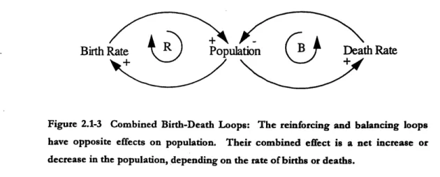
When combined (see Figure 2.1-3), the birth rate and death rate both affect population simultaneously. Simple mathematics shows a net increase or decrease in population as birth or death rates outpace one another. Note, however, that the system is dynamic. Fluctuations in birth and death rates simultaneously produce changes in
population, and a race between the two loops results in either a population increase or decrease over time.
Birth Rate ) opB Death Rate
Figure 2.1-3 Combined Birth-Death Loops: The reinforcing and balancing loops have opposite effects on population. Their combined effect is a net increase or decrease in the population, depending on the rate of births or deaths.
Although simplistic, this concept will be examined further as it relates to the
The balance between release rates and completion rates is considered work-in-process, or the "population" of material at any one time in the system.
As shown, a simple, first order system is easily determined. However, as additional variables are added to a system the results become much harder, if not impossible, to determine accurately. In the population model above, a myriad of other factors also influence population. Immigration rates, weather, food supply, disease, and medical
treatment are only a few factors that are included in a more complete model. As factors are added, the ability to simply balance rates of increase or decrease become increasingly
complex, and requires the aid of a model.
2.2 A Manufacturing Model
In a manufacturing environment, the factors affecting the "population," or inventory of a system are easily identifiable. The introduction of raw material, the completion rate, machine reliability, process time, supplier and process quality, and many other human factors contribute to the level of inventory. However, these factors are constantly changing - even by the minute - making a real time evaluation of inventory almost impossible. Again, a mathematical model can serve to aid in evaluating the performance of a system.
A note about data is required before beginning a discussion of modeling. The use of
computers in a manufacturing environment has contributed to incredible advances in
process efficiency and information and material flow. Automated production equipment has significantly increased the quality level of many manufactured components by eliminating countless sources of human error. These machines are also able to collect data many times per second, allowing continuous process feedback. Information systems provided up to the minute status of inventory that is readily available to all parties involved. These benefits come at a cost, however.
The sheer amount of data that can be collected has made analysis, in some cases, a nightmare. Although all parties involved in the system have access to the same data, the enormity can be overwhelming and analysis can be incomplete or even wrong. Computer systems that cannot communicate contribute to inaccuracies, and knowledge (or lack thereof) of statistical methods to synthesizing results contribute to flawed conclusions.
The point of noting the above costs and benefits is to further develop the need for a
replicate the performance of certain system characteristics to determine conclusions.
Forrester (1961) notes, "The key to success (in modeling) will lie in clear questions which are broad enough to encompass matters of major consequence but which initially limit a system
to proportions that fit the skill, time, and experience of the investigator" (p. 450). Modeling provides a systematic approach to simplifying the problem solving process by collecting only the data needed, and then using that data to come to a concrete conclusion not about the entire system, but about a specific issue or problem.
2.3 Industrial Dynamics
Jay Forrester, currently the Germechausen Professor Emeritus of Management at the Massachusetts Institute of Technology in Cambridge, Massachusetts, first studied these positive and negative effects as they related to industrial management in his work, Industrial Dynamics. The principles contained in this section will form a foundation upon which a model applicable to a specific manufacturing environment will be developed. In general, Professor Forrester provided a framework for studying information and material feedback systems, and the complex interrelationships between variable in such a system. He states
(1961):
Information-feedback systems, whether they be mechanical, biological, or social, owe their behavior to three
characteristics - structure, delays, and amplification. The structure of a system tells how the parts are related to one another. Delays always exist in the availability of information, in making decisions based on the information, and in taking
action on the decisions. Amplification usually exists
throughout such systems, especially in the decision policies of our industrial and social systems. Amplification is manifested when an action is more forceful than might at first seem to be implied by the information inputs to the governing decision
What makes this work so applicable to the problem identified in this thesis is that it incorporates many of the same variables one would encounter in a manufacturing system. Information and material flow are traced from an end-consumer back through retail, distribution, wholesale and manufacturing elements. As will be discussed in a later section, the model will not specifically note distribution, wholesale or retail segments. It will, however, use the same concepts to develop production process steps, inventory levels, and delivery to customers.
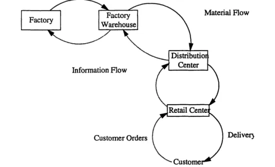
A schematic of Professor Forrester's system is shown in Figure 2.3-1.
ial Flow
Deliver)
Figure 2.3-1 Distribution Model Structure: This represents a four-stage distribution system where information (dashed lines) is transferred in steps from the end customer back to the factory, and material (solid lines) is then shipped forward to the customer. Delays in information and material flow are inherent in this type of system and contribute to the bullwhip effect. The bullwhip effect results in overordering back to the factory, expediting at the factory to meet customer demand, and then delayed shipment-of product at each stage forward.
Solid lines in the above diagram represent the flow of material from the factory through delivery to the customer. Dashed lines represent the flow of information from the customer order back through the system to the factory, where the product is ultimately produced. Delays are inherent in such a system. Rarely does a factory get simultaneous
information of a customer order, and rarely does a customer immediately receive an ordered product. Just as information has to pass through many levels between customer and factory, normally waiting for processing at each step, material follows the same hurry-up-and-wait path. Each level of the above diagram pushes to process orders and ship, but upon arrival at the next step, the material again waits in a queue for processing.
So what issues arise as a result of these information and material delays? Consumer data that is old contributes to a lag in responsiveness to customer needs. If the lag is only a few days, the factory has much more flexibility to adjust production levels to meet demand. As the lag increases, the factory is responding to consumer patterns that occurred sometime in the past. Additionally, if the cycle time of a product is considerable, or if the lead-time
from suppliers is long, the factory must hold much more inventory to maintain an adequate level of customer service. If the total lead-time is great enough and customers have to wait,
they may simply buy another product instead of waiting, even if it is of lesser quality
(although this is not typically the case in the aerospace industry, it should be noted). Finally, if the factory deals in products that are changing rapidly in the face of consumer needs or technological improvements, a long lead-time reduces the manufacturer's ability to get the right product to market to meet customer demand.
More importantly, not having real time information means that each level upstream of the customer must add a safety factor in adjusting to changing consumption patterns. For example, a sudden increase in buying means that a factory must immediately ramp up
production. As mentioned earlier, if the delay in learning this information is short, production schedules need only minor adjustment to make up for the increased demand. The time between the actual increase and the arrival of information at the factory means only a small number of backorders. If the time lag is great, much more time has elapsed allowing unfilled orders to increase. Then, when the factory receives the information, production must be dramatically increased. Unfortunately, in a system with both significant information and material delays two main consequences can result. By the time production catches up with demand, the actual demand has either decreased (leaving the factory with excess inventory), or customers have gone elsewhere to place their order (not only leaving the factory with excess inventory, but with lost orders in the future from customers who have lost confidence).
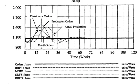
Professor Forrester's model, shown in Appendix B, mathematically models a system with multiple variables and significant delays, and two sets of results are shown. Figure 2.3-2
shows a one-time increase in demand, a "step," which is delayed as it moves back to the factory. Figure 2.3-3 shows cyclical demand, where the oscillation of demand at the consumer level multiplies as it again moves back to the factory.
Step
2,000 1,700 1,400 1,100 800 - Distributor Orders Production Orders -"""~-~- -f Actual Production RetailOrdr :'"-Retail Orders 0 12 24 36 48 60 72 84 96 108 120 Time (Week)Orders: base units/Week
RRF3:base --- -- -- units/Week
MOF3:base
---
---
units/Week
SRF3:
base
-
-.- -
...--..--.
----..
units/Week
RRD3: base - units/Week
Figure 2.3-2 Step Order Input: A one-time step perturbation is introduced to actual customer demand. The result is delayed orders from retailer to distributor (RRF) and from distributor to factory (RRD). Production orders at the factory (MOF) and then actual production (SRF) are further delayed. At each step, the order increase is exaggerated to meet the rise in demand. Each step must increase further than the previous step in order to meet both the original increase in demand and the buildup of backorders. Actual production peaks last and does not peak as high, since it is able. to see that demand is again level after the step input.
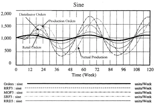
Sine
2,000 1,500 1,000 500 0 0 12 24 36 48 60 72 84 96 108 120 Time (Week)Orders: sine units/Week
RRF3:sine --- --- units/Week MOF3: sine --- --- units/Week
SRF3 sine - units/Week
RRD3: sine ..."... units/Week
Figure 2.3-3 Sine Order Input: A continuous oscillation is introduced to demand. As in the step input shown above, orders from the customer back to the factory, and then production orders at the factory, are exaggerated in amplitude and peak later than the original order curve. The order curves above appear to be headed out of control. If the oscillations in demand are great enough, this is precisely the result.
Note that each step up from the customer reacts to new information with more pronounced amplitude, and how each reaction peaks later than the previous step. This is known as the bullwhip effect, and it is common in many environments where the
distribution channel is extended in multiple steps, and where information is not immediately shared. The graphs above only show information flow from the customer to the factory, and do not show the delays in material flow as product moves from the factory to the customer. Below are the results of that material flow, again both with a one-time step input
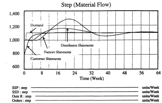
Step (Material Flow)
Demande D I istributor Shinmnts I actorn Shiment I I Customer SiDments I -0 8 16 24 SSF: step SSD: step Outs R: step Orders: step 32 Time (Week) 40 48 56 units/Week units/Week units/Week units/WeekFigure 2.3-4 Step Input (Material Flow): This shows the delays in material flow
from a one-time step input. Note that factory shipments peak much later and higher
than distributor or customer shipments as they try to catch up with backordered demand. Also, note that as shipments get closer to the customer they more closely
resemble actual demand, with customer shipments smoothly rising to meet demand
by Week 12.
Sine (Material Flow)
2,000 1,500 1,000 500 0 0 12 24 36 48 60 72 Time (Week) 84 96 108 120 SSF: sine SSD: sine Outs R: sine --- -Orders: sine units/Week units/Week units/Week units/WeekFigure 2.3-5 Sine Input (Material Flow): A constant demand oscillation is shown above. Again, customer shipments closely mirror actual demand, but factory
1,400 1,200 1,000 800 600 64 .
shipments follow demand trends in exaggerated shipments, peaking much later than the demand curve.
Here, note that again the curves peak higher and later for the distributor and for the factory deliveries, but the reasons are somewhat different from before. Here, it is shown that the retailers are much more responsive to customer changes. Their curve follows very closely with the orders curve and does not peak significantly higher. In the Step figure, the deliveries curve simply rises to meet demand, smoothly meeting it by Week 7. Curves for distributors and the factory, however, again show a delay in moving product to the next stage. Whereas in the first example the information was delayed telling each upstream step to order more goods and their successive orders curves peaked later, here the actual delivery curve peaks later. This is due primarily to the factory's ability to generate enough products to satisfy demand in the distribution chain.
2.4 Component Production and Engine Assembly
Why all the fuss about generic models, and what do retailers and distributors have to
do with manufacturing engine components? Actually, everything and nothing. The point of
this section was not to develop a model specifically of a distribution network. Instead, the purpose was to introduce a system comprised of many levels in a supply chain from the factory to and end-user, and to demonstrate the inherent material and information flow delays. Distributors and retailers deal in bulk shipments, not make-to-order turbine engines. They exist to make certain supply chains more efficient by providing an effective mechanism for material flow between the factory and customer. Turbine engines are make-to-order, are not shipped in bulk, and do not normally sit in inventory waiting for a prospective buyer. Therefore, there are no distributors or retailers in the industry. A shift will now be made from thinking of distributors and retailers as steps in a value chain to thinking of component production (furthest from the customer) and engine assembly (the last step before the
customer). Instead of now thinking of consumer goods moving through a distribution
network, now attention turns to an individual engine component moving from a manufacturing facility, through an assembly facility, then on to a customer. Information
flow from the customer to assembly, and finally to component production mirror orders for
consumer goods. At the same time, the movement of a component from production,
through assembly, and on to the customer represents the same material flow steps developed in the production distribution model of this section.
To further simplify this explanation, Figure 2.4-1 presents a schematic which highlights the similarity of the systems. Note that although fewer steps are shown in the engine model, the same information and material flow delays occur between the existing steps. Subtracting steps means that the furthest step away from the customer will see a smaller amplification of the original input, while adding steps further compounds the amplification. Again, dashed lines represent information flow and solid lines represent material flow. :WrFactory
Factory Warehouse
Distribution Center
Retail Centel)
4t
Customei 4Component Production
Assembly Warehouse
\AssemblyCente)
Engine Customer
Figure 2.4-1 Structure Similarity: The distribution model that is developed in this chapter is shown on the left. It is a multi-stage system of material and information flow. On the right, the manufacturing system studied in this research is also shown as a similar multi-stage system of flows. The interaction of multiple stages in systems such as these produce similar delays which affect material and information
flows.
The next chapter will develop a model similar to Professor Forrester's, and will speak more directly to the information and material flows between steps in a production and assembly value chain.
Chapter 3 Manufacturing Mode 1 Development
3.1 Analysis of Interviews and Data
Having motivated information and material flow thus far, and having introduced a technique for analyzing such issues, a procedure to integrate these factors and develop meaningful conclusions must be presented. Original work at the facility was accomplished by interviewing numerous individuals at various levels of the manufacturing organization. The goal was to understand the thought process - to understand the mental models
associated with solving similar problems - at all levels. Interestingly, the range of answers to particular questions relating to production schedules, production rates, orders and inventory varied widely from higher level executives to shop floor associates, even though the
questions were identical. Their mental models differed based on current information (both externally and internally obtained), historical experience at the facility, and breadth of knowledge of the entire system from raw materials to finished components and engines.
Given the foundation for a production model, attention now turns to its application to the manufacturing environment. As mentioned previously, the assembly facility receives both purchased and internally manufactured parts, then assembles those parts into either rebuild kits or complete engines, or consolidates them for spare parts shipments. This
model focuses on the movement of manufactured gears and shafts through the Case & Gear
COE and on to the assembly facility.
Originally, linking the Case & Gear COE with the assembly facility in a flow system based on customer demand of engine, kit and spares orders was the goal of the internship. A shift in manufacturing strategy of such magnitude required a high degree of employee involvement and management support. Also, it required absolute commitment to the principles of flow manufacturing as well as a commitment from suppliers for both delivery performance and quality. This system was not ready for such a dramatic change, so the goal was modified to present a feasible way to develop flow manufacturing within the framework of the current MRP system. Namely, to allow the Case & Gear COE to adopt a flow system independent of suppliers deeply rooted in MRP delivery and an assembly facility firmly committed to a production schedule.
Before suggesting improvements over the existing material and information flow structure, one must first understand the key drivers and metrics affecting performance of gear and shaft manufacturing and order assembly and delivery. This model was developed using Jay Forrester's model as a baseline, then adding key variables to first mirror historical data, then suggest why performance is affected. The process first identifies the key variables affecting the system and establishes a causal connection between these variables. Then a model is constructed that can be mathematically manipulated to explain the drivers and metrics. This final step, manipulation of the model, is where we are able to surface unanticipated side effects of management policies, then suggest ways to either rework or eliminate altogether these policies to drive intended behavior. A key deliverable of this process, given the management structure and existing production system, was to write a story that could be quickly synthesized and would naturally lead to possible solutions. The thesis, and indeed the entire internship serve to build system understanding of key drivers and dynamics for decision-makers so that system change can be enabled.
Numerous interviews were conducted at various levels of management, across
functions, and finally with shop floor employees. The method chosen was to start from the
top levels, then work down through the layers to where production and assembly was actually being accomplished. By using this interviewing approach, each story was either immediately reinforced or refuted, and key variables could be traced down through the system to learn policy impacts of behavior.
Once these variables were determined, they were separated into stocks and flows. These stocks and flows are simply defined as amounts that can be measured exactly at a given point in time (stocks), and rates that change over time (flows). Examples of stocks include work in process, unfilled orders, and finished goods inventory. At any given point in
time, the exact number of items in these stocks can be determined. Mathematically, stocks are simply the sum of flows entering and exiting, like water flowing into and out of a tub of water. If inflows are greater than outflows, the tub fills, and vice versa. Examples of flows are order introduction, delivery rates, component completion rate and assembly rate.
Although at any given point in time an exact number of items cannot be determined, the rate at which items are moving through the system can be. Mathematically, determining the rate involves taking the derivative of the completion curve, with the result (slope of the line) representing the exact rate.
The basic stocks in the system were easy to uncover. Completed engines, completed components, and work-in-process (WIP) levels for both formed the basis of most
interviews. Managers monitored inventory levels through reports for both work in process
and finished goods, and shop floor associates were keenly aware of the work waiting both ahead and after their manufacturing cells. Also, the Case & Gear COE tracked raw
materials, adding them as the third component of inventory. The stock of unfilled orders, or the number of gear and shaft orders placed yet still to be introduced onto the production floor, was noted and is important in a later discussion. Ironically, however, attempts were never made to mentally link completed orders and WIP with outstanding orders during the personal interviews, and an almost adversarial relationship existed between the enterprise, responsible for customer contact and maintaining order delivery, and production,
responsible for manufacturing the order components.
Flows in the system were also obvious, both for material and information. Goods moved from raw material into production, from production to the assembly warehouse,
from the warehouse into assembly or kit/spares orders, then finally on to the customer.
Although material flow through component manufacturing as well as flow through the assembly process will be linked and are included in the model, during this phase of development each process was assumed independent to avoid confusion and facilitate a complete understanding of each facility. Further analysis of each system showed that neither was truly optimized. Therefore, each system was identified separately as either Gear
Production or Engine Assembly, and independent average cycle times were used to compute
material flow.
Information flow occurred through both formal and information channels. Standard production and inventory information was readily available on an internal computer
network. Although read-write access to this network was extremely limited, anyone could easily review the data on a read-only basis. In parallel to this official documentation of
production and inventory transactions, an elaborate informal network between marketing
and sales, engine coordinators and production managers served to keep the system in balance on a more real-time basis. Although this informal channel created natural efficiencies, it is almost impossible to model due to its complexity and continual change. Therefore, the model deals only with the formal information channels to determine appropriate production rates.
3.2 Causal Loop Development
The basic causal loops started with component production and assembly. They highlight the difference between the number of components or engines to be completed in a time period and the actual number of pieces complete. This difference, or gap, forms the basis of an MRP system analysis, and provides a foundation for this model (Hopp &
Spearman, 1996). Original interviews uncovered a gap similar to this, occurring at the engine assembly facility, as progress was measured by comparing the number of orders complete in a week to the number of orders scheduled for completion.
Business cycles were measured in calendar quarters. Each quarter had production quotas for engines to be assembled and shipped, and kits and spare parts orders to be
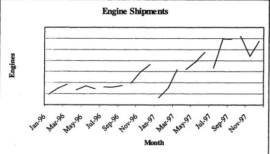
shipped. At the beginning of each quarter, employees noted that the shipment rate was slow and gained speed as the end of the revenue quarter approached. Data supported these assertions, and the shipment rates by quarter are shown in figure 3.2-1.
Figure 3.2-1 Quarterly Engine Shipments: Each short line shows the connection of shipment data from each three-month production quarter. For example, the first
connection of data points represent of January, February and March engine
shipment data. A deliberate break is made between the final month of a production quarter and the first month of the next to highlight the trend in rising shipments
within each quarter.
Engine Shipments
.. ..
,
,1 r44 9b
40
0\ ct\ , \The scale has been deliberately omitted, but the rising trend is clear by quarter. With the exception of the second quarter of 1996, the only outliers are in December 1997 and
1998. Holiday vacations severely decreased production time, and consequently less engines and kits were shipped.
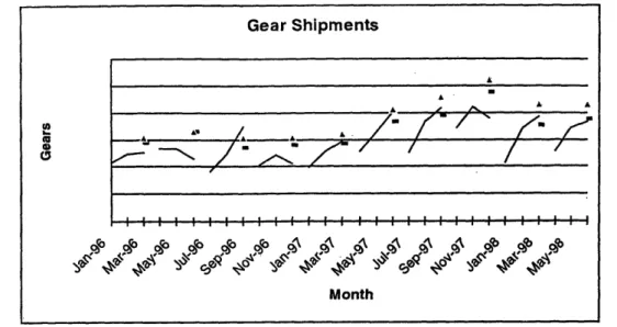
The next logical question was whether the Gear Production Center, linked to the assembly facility by its own production schedule for engine components, followed the same pattern. During almost every interview, the answer was a definitive "No, we produce gears and shafts at a constant rate." At first this seemed logical since the two facilities were physically separated, produced completely different products with different processes, and were under different management. Also, the volume of spare parts made the production rate seem more level. Data, however, refuted these claims and shows the same rising pattern through the quarter as the assembly facility (see Figure 3.2-2).
Figure 3.2-2 Quarterly Gear Shipments to Stores: As with engine shipment data, only shipments within each production quarter are connected to show the rising trend. Note the shipment decrease for December 1996, and December 1997. The drop in shipment levels reflects curtailed production due to holiday vacation.
Gear Shipments
io~~
Gear Shipments
Figure 3.2-3 Normalized Quarterly Gear Shipments: The solid lines are identical to the previous Gear Shipment figure. Here, however, additional data points have been added to answer the argument that the final month of a quarter contains five weeks instead of four. This is included to defend the rising trend.
Again, the scale has been omitted but the rising trend by quarter follows. As expected, this was a startling find for the Gear Production Center management, and many explanations for the behavior soon surfaced. First, it was argued that the first two months in each quarter contain only four weeks and that the third month contained five. Certainly this would explain the rise in the final month. Shown in Figure 3.2-3 are triangles and dashes at
each third month of the quarter. They are not data points, but instead represent a
normalization of data to account for the difference in weeks. The triangles show the
expected production rate in the third month if the second month shipments are increased by
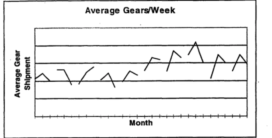
25% (to represent an increase from 4 weeks to 5). The dashes, to further show the failure of the argument, are the average of the first two months in the quarter, again increased by 25%. Next, it was argued that monthly totals did not accurately reflect a true production rate, and that possibly a weekly average would better show a flat production rate. Although this procedure does show a decrease in output/week (shown in Figure 3.2-4) during the last month of the quarter, the output/week statistic is meaningless. A per week statistic simply waters down the meaning of the initial data, measured on a per month basis, by dividing a rising total by a number 25% higher than that of month one or two, in cases where the total
LU b 9b 96 bA 5Aa A CA 4t 0 0 A A
... - , , ,'.
-:
i iS B I I I ! I II I I I I ! 1 111' 11
shipments did not increase by that amount. Our interest lies in the per month numbers, not necessarily in the average rate of each week.
Figure 3.2-4 Average Gears/Week: This figure represents the average number of gears produced each week during a production month. Since the last month of each quarter contains five weeks instead of four, the average is shown to decrease. However, this statistic is misleading in that total shipments for the final month still show a rising trend.
Attention now turns to establishing a causal relationship between the variables already mentioned, to gain an understanding of the system. First, the production and assembly gap will be developed in more detail, and then other variables deemed significant from interviews will be added. At each step, the causal loop diagram was presented to many of the people with whom interviews were conducted to maintain integrity of the story. The relationships that follow are the final loops developed during this phase in the model building process. For simplicity, only the assembly causal relationships will be developed. The production relationships are exactly the same, and will be further investigated when the two systems are linked.
As the assembly gap increases (again, the gap is defined as the difference between the
actual number of products complete and the desired number to be completed), pressure to
decrease that gap increases resulting in increased assembly. This loop is a balancing loop, where an increase in any variable contributes to a decrease in the production gap. They system tends toward zero to eliminate the gap. Two methods to relieve this production or assembly pressure were through normal assembly and overtime assembly (see Figure 3.2-5). Interviews with many shop floor associates supported this development. It was noted
Average Gears/Week a .0
a
w E-, en Month
without exception that the pace of shop floor activity increased dramatically as each month came to an end, with an even more significantly increased noted at the end of each
production quarter.
Complete Engines
Desired Engines
l +B
Normal Assembly
OTAssembly Asmbly
A
mbly Gap
'
)Assembly
PressuFigure 3.2-5 Production/Assembly Balancing Loops: These simple causal loops show the goal-seeking behavior of this production system. As the gap between desired engines and complete engines increases, normal and overtime (OT) assembly increase to drive this gap to zero. The (-) sign in the link between Complete Engines and Assembly Gap produce an opposite effect (increase to
decrease, decrease to increase).
By substituting gears or components for engines, an identical causal loop is constructed for component production. In both cases, a gap exists at the beginning of a production period between orders and complete product, resulting in pressure to fill orders. The stock of completed engines or components rise, the level of unfilled orders falls, the gap
approaches an equilibrium level of zero. The most plausible reference mode for this system is a linear increase in engines complete, stopping at the level of desired engines as shown in Figure 3.2-6.
Figure 3.2-6 Original Completion Reference Mode: The level of desired engines remains the same over the complete time interval. Completion of engines, theoretically, rises linearly to meet this desired level at the target time.
As discussed earlier, this was not the case in reality for the assembly facility. The curve began much flatter and rose aggressively as the end of the quarter approached and as pressure to complete engine orders increased (Figure 3.2-7).
Figure 3.2-7 Revised Completion Reference Mode: In reality, the number of completed engines rises exponentially to meet the desired number. Completion rates at the beginning of the time interval are very low, but increase dramatically toward the end.
Desired Engines
es
Completion Reference Mode
0.
.i53
0
C E0
0
Time
Revised Completion Reference Mode
U 0 10L. M0.a) E 0 C.
Time
-,a,.a = tOther variables were then added to the basic causal loops in order to determine the management policies which were really affecting assembly rates. The first and most
important policy was expediting engine orders as the quarter drew to a close. As can be imagined, as engines are expedited the problem works its way back up stream through the
component production centers and finally to suppliers, who must continue to supply raw
materials and purchased parts, but to a schedule which shows tremendous fluctuations. This, again, is the bullwhip effect.
How does expediting begin? What drives the decision to deliberately split a
production batch in order to speed it through the system? The answer to this question was not at all obvious but could be explained fairly easily after key interviews with engine assembly coordinators. The reason is that engines are started, or released to the assembly floor, even though not all parts necessary for completion are present at release. Associates at the assembly facility were very familiar with this behavior, as they saw engine and
subassembly carts wheeled to their stations every day without all necessary components. To the assemblers, the problem was that the carts were taking up space. To engine
coordinators, who's responsibility was to integrate both externally purchased and internally manufactured parts before release onto the floor, releasing without parts was the best way to get attention and action on the missing parts. Another reason given for starting engines without all parts was simply that the production schedule specified a certain release date, and that date would not be missed. Whatever the reason, as the quarter began more and more engines, kits and subassemblies found their way onto the assembly floor incomplete.
At some point during the quarter, the actual level of work in process became greater than the desired level for efficient assembly. This difference could certainly not be
determined exactly, but at a given time managers realized that shipments were behind, and the level of inventory on the floor was greater than necessary. What was the fix? Managers identified engines that could be completed within the quarter, then identified the parts necessary for completion, and finally either called external suppliers to add pressure to the order, or (as analyzed in this work) forced the component production centers to expedite critical components.
Does this sound inefficient? Certainly, but not because the managers aren't making sound business decisions. In fact, they are making absolutely correct decisions, but only as
they relate to their own piece of the system. Nahmias states, "If a sudden unusual event occurs, such as a much-higher-than-anticipated demand of a sudden decline in productive capacity.. .it is likely that many managers would tend to overreact" (p. 154). Unfortunately, an expediting decision of this type made very late in the manufacturing process (at assembly) has a great impact on all upstream steps and, as shown in the previous chapter, this effect is magnified at each level. The idea, then, is to understand both the cause and effect of such a decision at each level in the process in order to optimize the behavior of the entire system,
not just the behavior at one facility.
Finally, it was proposed that the primary objective of the system was to assemble and deliver as many engines and kits as possible during each revenue quarter, many times at the
expense of other orders. Early in the internship this proposition was refuted, but soon the
truth surfaced. On quotation in particular, received in an e-mail at the middle of one quarter, supported the original argument and led many managers to finally give up flawed mental models of system behavior. Quoted on October 15 as the Engines facility was making a final push toward end of year production quotas and revenue, "Also, please keep your focus on two things, the first being the close of the month for October is the 24h . Second, we must ship as many engines as possible by the 14h of November in order to have a positive impact on cash flow in the fourth quarter. Please target your delivery dates for the first week in November for all shipments, including both spares and engines that are
committed for the month of November." The original production schedule was being
abandoned, and any and all engines which could feasibly be completed in time to contribute to cash flow were identified and expedited.
How did this decision affect the component production facilities? Two weeks after receipt of the message above, another message was sent, but only to the component
facilities. "Please note that all serial numbers that are highlighted blue is what we must get out the door by Nov 14th for cash flow. Please focus on bringing in the controlling
hardware that falls within the blue highlighted engines. We need hardware no later than Nov 10th." Not only were engine orders expedited to meet delivery by mid November,
component facilities lost four additional days of production, and were still expected to
produce all necessary parts.
Let's again look at the bullwhip effect. After increasing the production rate at assembly a message is then sent to all component suppliers (both internal and external) to target parts delivery for November 10th.
Compared to the increasing slope of the assembly curve, to meet the same demand four days earlier required the component curve to rise even more aggressively, and due to the delay in information flow from assembly to components, it started to rise later.
The time is right to introduce the causal relationship of other variables noted in order to establish the cause and effect system leading to management decisions. As discussed earlier, the basic causal relationships are between the desired level of engines to be completed and the actual amount completed, and the
desired/actual number of components. Shown in Figure 3.2-8 are the causal loops for engine assembly. The loops for component production are identical, but they refer to components instead of engines. Later, they will be discussed together as the two systems are linked.
Complete Engines
Desired Engines
Normal Assembly
OT Assembly
Assembly Gap
Assembly Pressu
Assembly Pressu
Figure 3.2-8 Balancing Assembly Loop: These balancing loops drive the assembly gap to zero as the number of complete engines approaches the desire number.
As stated earlier these loops are balancing, forcing the engine gap to zero. Assembly pressure increases normal and overtime assembly, increasing the completion rate of engines, closing the gap between desired and actual number of engines for a given quarter.
Next, starting engines without all necessary components is included. In Figure 3.2-9, this variable is referred to as "Starts without Parts," which increases work in process in the engine facility and decreasing the rate at which engines are complete.
Desired Engines
ably Gap
Figure 3.2-9 Assembly WIP Reinforcing Loop: Assembly pressure forces engine coordinators to release engines onto the production floor without all necessary components. This increases WIP on the shop floor and decreases the rate at which engines are completed.
This new loop is a reinforcing loop, which increases the engine gap. As engines are started and WIP levels increase, the number of engines complete actually decreases.
Another reason stated for starting engines without all necessary parts was to gain attention for missing components. Engine coordinators, through past experience, realized that by simply starting an engine missing
parts, just to get it into view on the assembly floor, would add priority to those parts, requiring them to be
expedited, forcing more parts to assembly stores, and adding to the stock of complete engines. This new, balancing loop is shown in Figure 3.2-10.
Desired Engines
Assembly Gap
"II
Figure 3.2-10 Component Expediting Balancing Loop: The main reason given for starting engines without all components was to force attention to those missing parts. When attention on those missing parts increases enough, necessary components are expedited through the production system and more parts are shipped to assembly stores.
Finally, as managers note the increase in work in process levels, they are forced to identify engines which can feasibly be completed by the end of a quarter, and expedite them through the system.
Components
Component Shipments to Stores
Complete Engine ' Desired Engines
ibly Gap
Starts w/o Pats
Figure 3.2-11 Engine Expediting Balancing Loop: An additional dynamic is observed at engine assembly. As WIP in the assembly facility increases, managers identify engines that can be expedited to decrease WIP. Expediting engines results in more· component expediting.
This forms a new loop, shown in Figure 3.2-11, a balancing loop that again tries to decrease the engine gap to zero. If we look at only the assembly facility, four separate variables are affecting the system -normal assembly, overtime assembly, starts without parts, and expediting. As each of these is introduced,
trying to predict which variable will have the most profound impact becomes much more complex. Hence, the necessity for this type of modeling. Additionally, when the two systems are linked, there are many more variables racing to either increase or decrease the engine and production gaps.
At this point, the systems must be linked and all necessary variables included to develop a complete picture of the assembly-production system. Presented in Figure 3.2-12 is the entire causal loop system for assembly and production, linked as appropriate, including all variables noted in interviews and research. The following section presents a much more detailed mathematical formulation supporting the model calculations.
-C r Asewtr!blr >-':4 Pructionc
Actual Revenue
Spare Paris Shipments Engine Shipments
Revenue Gap
Desired Revenue
pare Parts
Figure 3.2-12 Complete Causal Loop Structure: Above is the combination of all variables in their appropriate causal loops. Engine assembly, component production and expediting are all included to portray all the dynamics of this system.
First, the revenue gap determines the desired number of engines and desired components (desired
components being the sum of rebuild kit orders and spare part orders). The number of engine components is
added to the Desired Parts to Stores through the variable Desired Engine Parts. The two systems are then linked through the variable Desired Parts to Stores. Tlis is the number of internally manufactured
components that the assembly facility needs to complete engines and fill kit and spare part orders. As the relationship continues, components are manufactured and Parts to Stores feeds back into Normal Assembly and Spare Parts Shipments, completing the cycle.
Next, attention turns to the other key variables noted, namely Starts without Parts and Expediting. Assembly pressure drives both of these variables, resulting in increased WIP and increased pressure to decrease WIP. Again, the loops continue in both cases through parts to stores. But where does this pressure come from?
Pressure in both assembly and production comes from the variables Engine Time to Target and Gear Time to Target. Mathematically, as the time to target decreases, a corresponding increase in pressure is seen.
Although as time decreases pressure should increase linearly, in reality the time decrease is linear and the pressure increase is exponential.
Though the quotations noted above were obtained well after this system-wide study was begun, all preparation led to a problem statement. This statement had to be broad enough to include all variables noted during interviews, yet specific enough to provide solid direction for the model. Our interest is not necessarily to model the entire system, but to model the relevant factors affecting a problem in order to understand the time varying relationships between parts of a system which directly impact the specific problem.
The problem statement evolved as follows. Expediting engines through assembly and test negatively impacts all component production by increasing schedule disruption, where ultimately the benefit of shipping incremental engines is outweighed by the cost remaining work-in-process. The quotations noted above, when they were made, only added support to the problem statement, and provided the impetus for further study.
3.3 Model Development
Once the causal relationships were agreed on, and the problem statement was
approved, attention turned to developing a mathematical representation. In the loops above, revenue drives initial engine and parts schedule demand. While in reality this was true, it was not necessary to include this variable in a model that represented only one quarter. It
seemed more straightforward to assume a certain number of engines for a quarter, based on historical data, then develop the model to mirror historical behavior in relation to the specified production and assembly quotas. Additionally, this model was not meant to show system reaction to a variety of engine order inputs, but rather to show system reaction to a chosen input, based on a variety of combinations of internal variables.
For simplicity, models for component production and engine assembly will be developed individually. Then, once the similarities and differences between each independent system are understood, they will be linked to show the complete flow of
components through production and assembly, then on to the customer.
The stock of unfilled orders (UO Gears) begins the gear production model (see Figure 3.3-1). This represents the stock of outstanding orders awaiting some element of administrative processing, and which have not yet been introduced into production. This stock is increased by incoming orders for gears and shafts (Gear Inc), both from OEM