Air traffic control using Virtual Stationary Automata

Air Traffic Control Using Virtual Stationary Automata

by

Matthew D. Brown

B.S., Massachusetts Institute of Technology (2006)

Submitted to the Department of Electrical Engineering and Computer Science

in partial fulfillment of the requirements for the degree of

Master of Engineering

at the

MASSACHUSETTS INSTITUTE OF TECHNOLOGY

September 2007

©

Matthew D. Brown, MMVII. All rights reserved.

The author hereby grants to MIT permission to reproduce and distribute publicly

paper and electronic copies of this thesis document in whole or in part.

Author .. ...

...

Department of Electrical Engineering and Computer Science

June 8, 2007

Certified by...

...

Nancy Lynch

Professor of Electrical Engineering and Computer Science

Thesis Supervisor

Accepted by .... ... . 1 Ls,. . .••.~...

Arthur C. Smith

Chairman. Denartment Cnmmittee on Grrduaitp ,tllSdpnt. MASSACHUSETTS INSTITUTR

OF TECHNOLOGY

OCT 0 3 2007

LIBRARIES

ARCHIVES

Air Traffic Control Using Virtual Stationary Automata

by

Matthew D. Brown

Submitted to the Department of Electrical Engineering and Computer Science on June 8, 2007, in partial fulfillment of the

requirements for the degree of Master of Engineering

Abstract

As air travel has become an essential part of modern life, the air traffic control system has be-come strained and overworked. This problem is occurring because the capacity of the current air traffic control system is severely limited by the capabilities of its human operators. There-fore, if we are to increase the capacity of the air traffic control system, then we must develop new automated systems for air traffic control.

In my thesis, I take a distributed approach to automated air traffic control. I use a wireless ad-hoc network to simulate a layer of Virtual Stationary Automata, or VSAs, which are virtual machines located at fixed locations in space. These VSAs can then be used to help coordinate the aircraft in the air traffic control system.

I model the air traffic control system as a directed graph, showing how the continuous real world air traffic can be abstracted into a discrete graph representation. Using this graph rep-resentation, I provide two algorithms to perform safe and efficient air traffic control and prove their effectiveness.

Thesis Supervisor: Nancy Lynch

Acknowledgments

I have received an amazing amount of help in various forms from innumerable people during the writing of this thesis and throughout my time at MIT, and would like to recognize a small number of the individuals who helped make it all happen.

First, I would like to thank Nancy Lynch, who, aside from introducing me to distributed algo-rithms during a summer UROP years ago, has been dedicated to excellence in every step of the thesis writing process. Without her help and insight, this work would have lost so much of its technical rigor and clarity, and for that I am immensely appreciative.

I would also like to thank the rest of the Theory of Distributed Systems group that I have had the pleasure of working with these past couple of years. I would especially like to thank Tina Nolte for her extraordinary help throughout the process of the development of my algorithms in this thesis, and for giving me a solid base of research to model this thesis upon. Also, Seth Gilbert and Calvin Newport were extremely helpful while working on the VN Simulator, and without that work this thesis never would have happened.

My parents and family have been extremely supportive of me, and without that support and the strong value placed on education that they have instilled in me since childhood, I never would have been able to get this far.

And finally, I would like to thank Elizabeth for her constant emotional support, and for always being the one I can talk to about anything and everything.

Contents

1 Introduction

1.1 Outline of the Thesis . 2 Background

2.1 AirTraffic Control ...

2.2 Distributed Algorithms and Virtual Stationary Automata .

2.4 Chapter Summary... 2.5 Global Constants ... 3 The Physical Network Layer

3.1 Architecture of the Network La: 3.2 Aircraft -The Physical Nodes . 3.3 Communications - The Bcast S 3.4 RealWorld ...

3.5 The Physical Layer... 3.6 Chapter Summary ...

yer .

ervice . . . .J

Continuous VSA Layer Regions ...

Architecture of the VSA Layer Clients ...

Virtual Stationary Automata . Intraregional Communication 34 . ... ... ... .... .. .. ... ... .. ... .. 35 . ... ... ... ... ... .. ... ... ... .. .. 36 . ... ... ... .... .. .. ... ... ... ... . 39 . ... ... .... ... .. ... .. ... ... ... . 40 - Bcast . . . .. .. . . . 41 4 The 4.1 4.2 4.3 4.4 4.5 ... ,.,. ...

...

...

4.6 4.7 4.8 4.9 4.10

Interregional Communication -VtoVcast . . . RealWorld ...

The Continuous VSA Layer... Emulation of the VSA Layer ... Chapter Summary ... 5 The Known Path Model

5.1 Architecture of the Known Path VSA Layer 5.2 Graph Representation and Regions .... 5.3 GraphRealWorld ...

5.4 The Known Path VSA Layer ... 5.5 Bounding Areas ...

5.6 Arranging the Bounding Areas... 5.7 Emulating the Known Path Layer with the 5.8 Chapter Summary ...

6 The FIFO Algorithm

6.1 Problem Specification ...

6.2 Capabilities of the Known Path VSA Layer 6.3 Algorithm ...

6.4 Proofs of Safety and Progress ... 6.5 Chapter Summary ...

7 The Heuristic Priority Algorithm

7.1 Efficiency in a Free-Flight System ... 7.2 The Time to Arrival Heuristic ... 7.3 Algorithm ... 7.4 Chapter Summary ... .. ... .. .. ... .. ... ... . 42 .. ... .. .. ... .. ... ... . 44 .. ... ... .. .. ... ... .. .45 .. ... ... .. .. ... ... .. .45 ... .. ... .. ... ... ... .. 46 . . . . . . . . . . .. . . .

...

...

...

...

...

...

...

-. -. -. -. -. -. -. -. -. -. -. -. -. -. -.

...

...

...

8.3 Closing Comments .... . ... ... ... 105

9 Appendix ₁₀₇

List of Figures

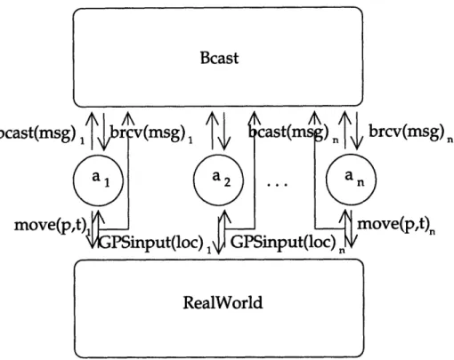
3-1 Architecture of the Network Layer for I = {1, 2,...,n} . ... 23

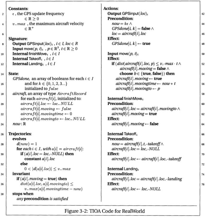
3-2 TIOA Code for RealWorld ... 30

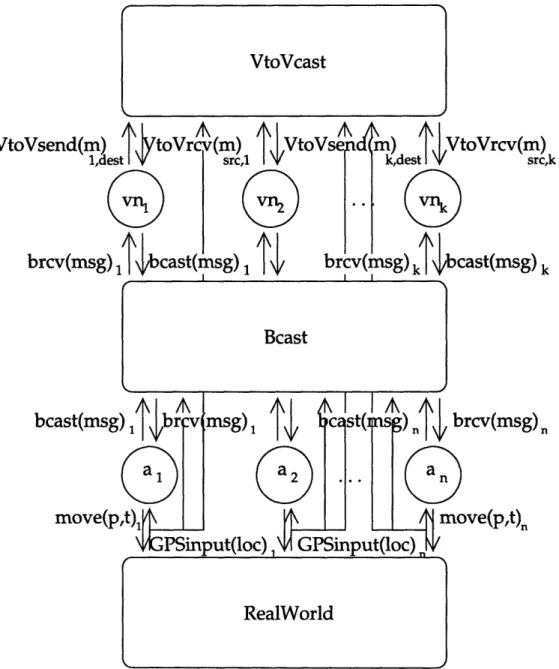
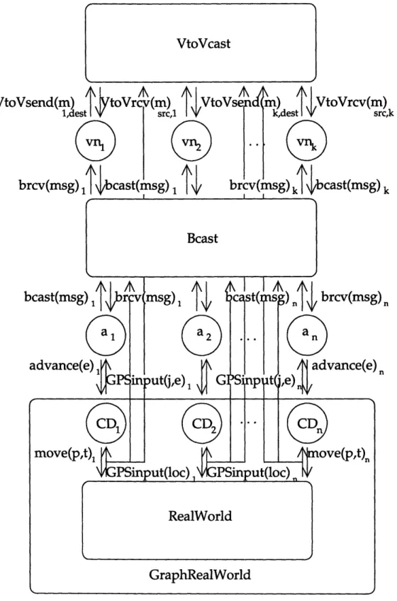
4-1 Architecture of the VSA Layer, for I = {1, 2, ..., n} and J = {1, 2, ..., k} ... 37

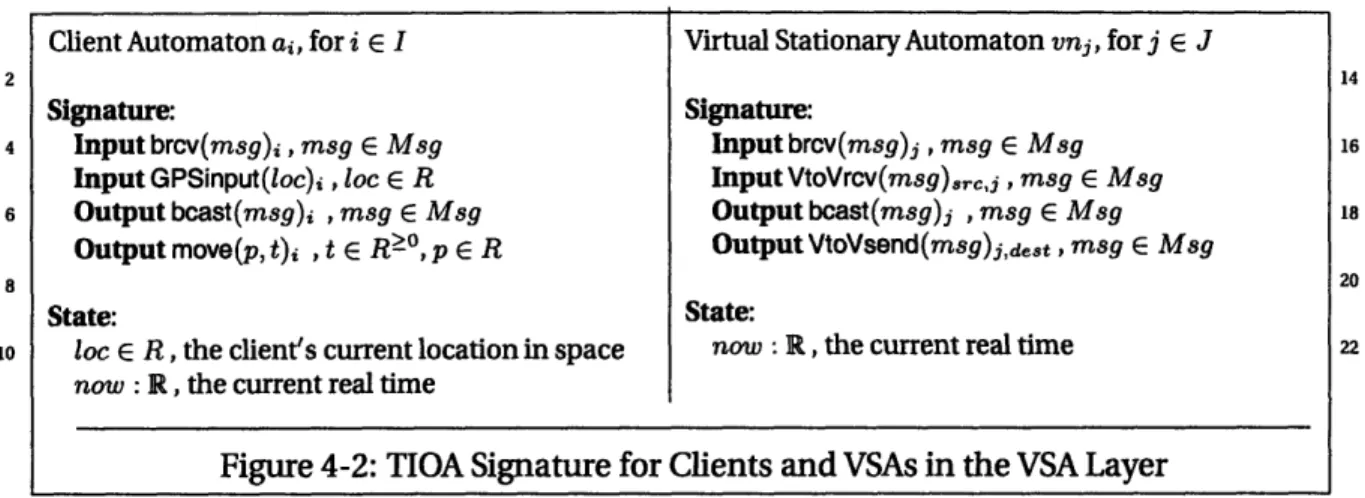
4-2 TIOA Signature for Clients and VSAs in the VSA Layer . ... 38

5-1 Architecture of the Known Path VSA Layer, for I = {1, 2, ..., n}, J = {1, 2, ...k} . ... 50

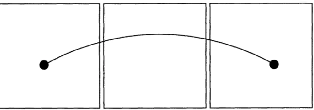
5-2 A Constraint on the Layout of Vertices and Regions . ... 52

5-3 TIOA Code for GraphRealWorld ... 54

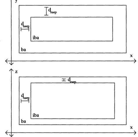
5-4 Cross Sections of Bounding Area ba and Inner Bounding Area iba ... 64

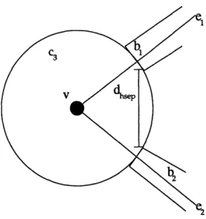
5-5 Bounding Boxes bl and b2 Meeting at Bounding Cylinder c3 . . . 66

5-6 Emulation of the Known Path VSA Layer, for I = {1, 2,...n}, J = {1, 2,..., k} ... 68

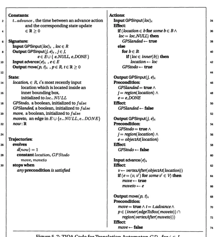
5-7 TIOA Code for Translation Automaton CDI, for i E I ... 70

5-8 TIOA Code for RealWorld with Graph Constraints ... 72

6-1 TIOA State for VSA vnj forj e J ... 86

6-2 TIOA Actions for VSA vnj for j E J ... 88

6-3 TIOA Code for Client Automaton ai for i E I ... 90

7-1 TIOA State for VSA vnj for j E J ... 99

Chapter 1

Introduction

As air travel has become an essential part of modern life, the air traffic control system has be-come strained and overworked. Frequency and routing of flights are often limited by the ca-pabilities of the modern air traffic control system, and the problem is getting worse every year. Compounding the problem, demand for a new class of very light aircraft threatens to further clog the system, rendering it ineffective.

The most significant reason for this capacity problem is the fact that ATC has not evolved as air travel has grown. While the tools and systems have improved with modem technology, the system is still limited by the capabilities of the air traffic controllers that operate it. Therefore, in order to adapt the air traffic control system for the demands of the coming years, we must begin to devise automated systems for air traffic control.

My approach, detailed in this thesis, uses distributed algorithms to allow aircraft to control themselves, without the need for a fixed air traffic control infrastructure. There are many ad-vantages to this approach: the computing and communications hardware are already installed on the aircraft; no expensive new infrastructure needs to be deployed for the system to work; and the system can be deployed in locations where it is either too costly or simply impossible to install static infrastructure. That said, without static infrastructure, many difficulties and com-plexities arise, which must be accounted for in the interest of safety.

At a high level, my method is to utilize a wireless ad-hoc network to implement a number of Virtual Stationary Automata, a system which simulates reliable virtual machines at specific

these virtual machines reliably. Using these virtual machines, distributed solutions to problems become much easier, as I can rely on these virtual machines as a point of communication, data storage, and decision making.

1.1 Outline of the Thesis

I will begin in Chapter 2 by discussing the background of the research. First, I will summarize some of the current practices in air traffic control at a relatively high level so that the reader can be properly introduced to the issues at hand. Next, I will introduce the theoretical concept of Virtual Stationary Automata (VSAs), and the relevant work done in the field. After that, I will connect the two topics, explaining how the concept of Virtual Stationary Automata can be used to help create an algorithm for air traffic control.

After completing discussion on the background of the research, I will present a series of mod-els for the network layer of the system. In Chapter 3, I will specify the capabilities of the aircraft and the capabilities of the wireless ad-hoc network which will be run on the aircraft. Then, in Chapter 4, I will specify the VSA layer, a virtual networking layer that runs on top of the physical network. Throughout these two chapters, I will make appropriate assumptions which will allow us to get to the core of the problem and avoid being concerned with extraneous details of the

operation of the network layer and emulation of the VSA layer.

I will then provide a model for the system called the Known Path Model in Chapter 5. The model will represent a limited free-flight system of air traffic control. This means that there are a number of predetermined paths through airspace that must be followed, but the pilot can inde-pendently choose which of these paths to follow. I will begin by providing a modified VSA layer which contains a representation of this model. Then, I will describe the physical world that the system will run in, and explain how the physical world is abstracted into a graph representation to represent the known paths.

After that, I will specify two algorithms for air traffic control using the Known Path Model. This first, presented in Chapter 6, will be called the FIFO Algorithm, named for its handling of conflicts using a queueing system. It will focus on keeping the aircraft safely separated from one another. The second, presented in Chapter 7, will be called the Heuristic PriorityAlgorithm, and it replaces the simple queueing system with a method for heuristically prioritizing aircraft when

conflicts arise. It will focus on efficiently moving the aircraft to their destinations while ensuring that the separation requirement still holds.

Finally, I will briefly discuss where this research leaves us, and make some suggestions on future avenues of research that would be interesting, ending with my conclusions about the algorithms provided within.

Chapter 2

Background

In this chapter, I will discuss the background of this research into a distributed algorithmic ap-proach to air traffic control. I will begin by giving a short primer on the current system of air traffic control, how it works, and some new developments in the area. I will then proceed to discuss ad-hoc networks, some recent research, and how the research led to the formalization of the Virtual Stationary Automaton. Finally, I will present some previous work with Virtual Sta-tionary Automata, showing how the concept can be applied to my goal of designing an air traffic control system.

2.1 Air Traffic Control

In order to understand the problem domain, a brief history of the current system of air traffic control (ATC) will be helpful. The majority of the information in this section on the history of air traffic control, and the current air traffic control system can be attributed to either texts on air traffic control, such as Nolan [9], or to general information encyclopedias [10,11].

In the earliest days of flight (before the 1930s), air travel was primarily performed during the day under clear visibility conditions. Because the traffic was so visible and there was so little of it there was no need for an organized system of air traffic control; safety could be left up to the pilots. When airplane instrumentation evolved to allow safe control of flight without having good visibility, a new set of rules for flight called instrument flight rules (IFR) were developed. This introduced the problem that pilots were able to fly without being able to see other aircraft

in the sky. As IFR flight became more common, and pilots started flying in increasingly hostile conditions, the need for a formal system of air traffic control became obvious.

2.1.1 Structure of the ATC System

Although the technology has evolved significantly in the past few decades, the system of air traf-fic control currently employed in the United States and around the world is quite similar to the system implemented in the mid 1960s. The airspace is divided up into a number of parts each of which is independently controlled. A plane flying from one part to another is passed off between the authority in one part to that of the next part so its route can be continued safely. We examine the way that the US airspace is divided up as a start of our discussion of ATC.

The United States airspace is divided up into twenty-one zones called centers. Each center is run by an Air Route Traffic Control Center (ARTCC), which manages the airspace of the entire center except for small areas of airspace around airports. Each center is then divided further into a number of sectors comprising most of the airspace in the center, and a small number of special portions of airspace around some airports called Terminal Radar Approach Control (TRACON) airspace. The TRACON airspaces are monitored by special facilities, while the sectors are monitored by the controllers in the ARTCC.

Within each ARTCC, aircraft in each sector are monitored and separated by a controller re-sponsible for that individual sector. That controller instructs each pilot how to remain safely separated (either horizontally, vertically, or both) from other aircraft in the area. If congestion in the area gets too bad, airplanes can be forced into a holding pattern, staying in a sector until the congestion subsides and the air traffic controller allows the pilots to continue along their route.

2.1.2 En-Route Control

One of the most conceptually difficult matters of air traffic control is the handoff of a plane between controllers when a plane moves from one sector to another. How do the controllers seamlessly transfer a plane's information from one to another, ensuring that there will be no problems?

Each plane has a flight progress strip which includes all the necessary data for tracking the flight. These strips are either on paper or electronic, and they get passed between controllers,

and between ARTCCs, as the flight progresses. Adjacent ARTCCs have Letters ofAgreement with one another, dictating appropriate altitudes and locations for planes to fly in when passing be-tween the centers. Within each ARTCC, controllers of adjacent sectors also have agreements similar to the Letters of Agreement between the ARTCCs. But when special circumstances arise, it is up to the controllers of each sector to maintain proper separation when a plane transitions between them.

Other than the transitions, the en-route control of an aircraft, or the control that occurs while flying between airports, is relatively straightforward. Controllers keep the planes in established airways, depending on the origin and destination of the flight, and make sure the plane is using the correct altitude, heading, and velocity to remain separated from other aircraft in their sector. This separation must conform to the FANs minimum of (under normal conditions) 1000 feet vertical separation or 3 nautical mile horizontal separation. Changes occur sometimes due to bad weather or turbulence in which case the pilot may request changes in altitude or course, and the controller must make sure that these changes will not result in any of the rules of separation being violated. Weather and traffic can also cause the controller to redirect or hold an aircraft in a specific sector, although this holding is much more commonly done in the area around the destination airport.

2.1.3 Terminal Control

The other half of the air traffic control equation is called terminal control, in which the takeoff and landing patterns of the aircraft are determined. These are the functions performed by the special portions of airspace at either the TRACON facilities or local airports' tower operators. This terminal control also covers control of the runways, taxiways, and terminals: including both planes and airport ground vehicles. This takes place in TRACON facilities, using radar and the other electronic monitoring technologies that are in place at the airport. Terminal control also takes place in airports' control towers, which use electronic tools as well as visual identification of aircraft and vehicles to control the local area.

2.1.4 Looking Ahead

As I stated earlier, the system that was in place nearly forty years ago is very similar to the system that is used today. This is problematic for a number of reasons. First of all, the sheer volume of air traffic has increased so much in that time that the old methods may not be as useful to provide safe control of the increased number of aircraft that are now operational. Second, the technology level has increased rapidly in that time, and the current system is having a hard time catching up. While many new technologies have been added to the ATC system in the past forty years, the overall workflow is very much the same, and it may be a limiting factor to the technologies' integration. For example, the recently developed Traffic Collision Avoidance System (TCAS), which alerts pilots to possible collisions and instructs them to adjust course accordingly, has caused a small number of in-air collisions or near misses when the TCAS and the local air traffic controller gave pilots conflicting instructions.

From an efficiency perspective, the rigidity of the current system wastes a lot of resources; certain airways might be reserved for a certain pattern of traffic that is not occurring at that mo-ment, but could maybe be used for a different pattern of traffic to relieve temporary congestion problems. Limitations of human controllers have led to a very rigid framework, in order to make the traffic control problem manageable for controllers.

In an effort to help alleviate these limitations, institutions such as NASA, working with the FCC[14], are developing systems to return the air travel community to a system of free flight, allowing pilots to control the course of their aircraft without the need for en-route ATC. Using the new systems being developed for discovering nearby aircraft, avoiding mid-air collisions under IFR conditions is now possible. Using the current system, a lot of our airspace is wasted due to a lack of controllers for all sectors. Free flight could allow pilots to utilize the entire airspace, but may cause serious problems in heavily congested areas around major flight routes.

Advances in computing and technology, though, can now allow individual aircraft to coordi-nate with other aircraft to perform air traffic control in a decentralized manner. By developing a new system to ensure air safety, the human errors involved can be minimized and the volume of air traffic supported can be increased significantly while maintaining or improving safety. A hybrid system, somewhere between the free flight system and the current ATC system, seems to be the most likely candidate for use.

2.2 Distributed Algorithms and Virtual Stationary Automata

Now that we have an understanding of the air traffic control system that is currently in place, the methods for developing an algorithm to control air traffic can be explained in detail. While there is a large amount of research going on in the creation of a number of new next-generation air traffic control systems, this research will take a different stance in that it will be primarily a distributed algorithm, one that needs little or no centralized control, and that could theoretically be run using only hardware similar to that already installed in modern aircraft.

2.2.1 Wireless Ad-hoc Networks

The current system of air traffic control and its communications features comprise what is called

a basestation-type wireless network. While communication between an aircraft and the ATC

center is done through a wireless signal, the infrastructure of the network (the ATC centers) is static. The task of coordinating the large number of aircraft in the area becomes (at a high level) an aircraft asking the center for instructions, the center analyzing the data that is available to it in order to make the best decision, and the center replying to the aircraft. This system has a great benefit in the static nature of the center: the aircraft always know where and how to reach each center as they travel, and the center will always be there to respond to the aircraft. That benefit can also be a detriment, though, when we realize that this single static ATC center can become a bottleneck or a single point of failure if problems were to arise.

Therefore, we will consider the case where this is no static physical infrastructure in our com-munications network. Without fixed infrastructure, we are left with a large number of mobile physical nodes (aircraft), which may be entering and exiting sectors constantly and entering and leaving communications range with other aircraft without significant warning. This type of network topology comprises a wireless ad-hoc network, one that gets created by the combined capabilities of the clients in range of one another.

An ad-hoc network has a complementary set of problems to those of the basestation-type network: there is no static node to interact with. For example, a plane flying into a sector con-trolled by an ad-hoc network can see a completely different set of network connections every time it enters the network.

and safely coordinate with other clients, but without the benefit of a reliable controller to interact with. This problem is an important concern in research into distributed computing over ad-hoc networks.

2.2.2 Earlier Work in Ad-hoc Networks

To solve the problem, we can consult a great deal of recent previous work in the area. A naive approach to coordinating over a wireless ad-hoc network could attempt to treat communication similarly to a wired static ethernet, discovering the other computers which could be reached by the communication link, and communicating until the link was broken due to movement or failure. It would be impossible to tell when a link was likely to go down, as the wireless ad-hoc network contained no information about the relative locations of the clients to one another.

By adding the use of geographical information into the system, though, the highly dynamic nature of the network becomes more predictable. If each client has the ability to determine its location through a service such as the Global Positioning Satellite (GPS) system, the local network topology becomes easy to examine at any time. A theoretical client on this network could use the geographical information to make important decisions about whether another client is likely to be in communications range in the near future, or coordinate behavior with other clients based on their locations. Under the assumption that clients have access to this geographical information, the possibility arises for reliable algorithms to coordinate clients on an ad-hoc network.

An interesting problem in distributed computing is to provide a long-range routing service over an ad-hoc network, in order to transmit data wirelessly further than could be done over a single link. Algorithms such as GeoCast [5] and GOAFR [4] both use the location of the clients to provide a mobile routing solution. Each client can determine which of the others in com-munication range is most likely to be able to continue the transmission of a message to a given location, and could therefore pass the message to that client, who would continue to pass it until it either reached its destination or the destination is determined to be unreachable.

Another problem is more local: storing data in a certain geographical location so that any clients who come within range will have access to it. Storing the data on an individual client could not in itself work, as that client may leave the area where the data needs to remain. A

proposed solution to this problem by Dolev, Gilbert, Lynch, Shvartsman, and Welch is called Geoquorums [1]. As the name suggests, the algorithm uses geographical information to achieve agreement between a number of clients: specifically, to solve the aforementioned problem of storing atomic data reliably in a specific location without any static infrastructure to store the data on.

The key idea of Geoquorums is that it uses an emulated virtual machine to store this data. Clients on the network are therefore able to communicate with a single static machine in a spe-cific location, and do not have to worry about the dynamic nature of the ad-hoc network. The algorithm was not originally very reliable, as once the data storage point failed, clients were never able to recover the lost data. This problem has since been rectified by Tulone [18] using a slightly changed implementation and set of mobility constraints to guarantee data availability.

Work has also been done by Dolev et. al. [15] on Virtual Mobile Nodes, which were given the ability to change position along preplanned trajectories. Virtual Mobile Nodes were formalized as simple Input/Output Automata (or I/O Automata) [16, 17] and they could take an input, pro-cess that input, and provide an output. While they still had a virtual location in space, they were mobile, not fixed as Virtual Stationary Automata would be.

2.2.3 Virtual Stationary Automata

As previously stated, I use Virtual Stationary Automata in this thesis, an idea which drew influ-ence from the work mentioned in the last section. Virtual Stationary Automata [3,7,8] are fixed in space as in the Geoquorums work, can react and process information like the Virtual Mobile Nodes, but are given access to not only a GPS service, but a real-time clock service as well.

A VSA is a Timed I/O Automaton [19], with access to a real-time clock and a local broad-cast service allowing it to communicate with clients in its region and VSAs in the neighboring regions. The mobile physical nodes in an ad-hoc network emulate this machine, but how does this emulation of the VSA work?

The idea behind the VSA is to separate the total area of the network into some number of

regions. Within each region is a Virtual Stationary Automaton (also known as VSA or virtual

node). For simplicity, we can consider the center of the region to be the point that contains the VSA. We choose the size of the region such that under normal operation, any physical node

within the region will be able to communicate with any other physical node within that or a neighboring region.

The physical nodes within each region do the work to emulate the VSA within the region. A physical node is elected as leader to act as the node that actually sends all communication from the VSA of that region, and to handle the arrival of new physical nodes. To achieve fault-tolerance in the maintenance of the VSA state, the state of the VSA is replicated at some number of physical nodes in the region.

All communication within a region is done through broadcasts, allowing all physical nodes in the region to receive the message. If the VSA needs to send a message, the leader performs that send function. When the leader leaves the region, a new leader is elected to take its place, and since the other physical nodes have seen the same messages as the leader, no state should be lost. When a new physical node enters the region, the leader sends the state of the VSA to it so it can start emulating the machine at the same point as the rest of the physical nodes.

The VSA has become an effective framework for writing distributed algorithms. A number of papers have been written building on the work done in formulating the VSA to perform a wide variety of coordination tasks [7,8,12,13]. One algorithm uses VSAs to coordinate the motion of mobile devices [7], instructing clients to go where they are needed to fill in an area on a curve in space. Another set of algorithms [8] solves the problem of routing messages between clients over long distances using a multitiered approach. First, a service is created to route a message to a certain location in space. Second, a service for locating clients in the global network is created, using a VSA at the client's home location to keep track of the client's current position. Using those two services, a client-to-client message routing service is created, allowing messages to be routed over long distances without the use of static infrastructure.

Some work has also been done to expand the VSA out of the theoretical realm [12, 13]. A framework for running a restricted version ofVSAs has been written in Python and run on mobile devices. Programs for both the client and the VSA can be plugged into the system, allowing it to perform virtually any task that a non-timed, reaction-based VSA system can do. A simulation of a traffic light in space was implemented and tested, using the mobile devices to display the state of the light. This, in a preliminary way, is one of the main inspirations for the upcoming work in air traffic control. While there are currently no plans to implement the proposed ATC system,

the fact that it is possible in the future certainly is interesting.

2.3 VSAs and Air Traffic Control

In the previous section, I attempted to give some background on the concept of Virtual Station-aryAutomata, but I have not yet discussed exactly why the concepts behind the VSA fit the prob-lem of air traffic control so well. By connecting the probprob-lem of air traffic control to the theory of VSAs, it becomes clear why this research is interesting from two perspectives: the perspective of someone looking for a novel method of air traffic control, and the perspective of an algorithms researcher looking for interesting new ways to use VSAs.

The specific problem that I am solving is the modeling of en-route air traffic control using VSAs. The problem of terminal control is separate, and will not be covered. While this will be a theoretical treatment of the problem, the goal is to make reasonable assumptions about the sys-tem, keeping it similar to the real world. I will also justify a number of simplifying assumptions, which should allow readers from both theoretical and programming backgrounds to understand the algorithms presented.

While the current air traffic control system has been around for a long time, a distributed approach such as this has only been conceived of recently, for a number of reasons:

* Until recently, the ability to have enough computing power to run an air traffic control algorithm locally on all aircraft was not possible. While large jet liners have had significant computation power for years, these large aircraft are not the only aircraft in the sky. A complete air traffic control system must also work with smaller, single-engine aircraft. One could easily implement this system on modern laptops or small devices stored in even the smallest single-engine aircraft.

* The invention and refinement of the GPS system has allowed aircraft to have detailed and accurate information about their position without using ground-based radar. If the radar of an ATC center were necessary to position the airplane, there would be little reason to distribute control of the air traffic -the infrastructure would be necessary for the operation of the system. But since each aircraft now has the ability to determine its own position, we can think about the possibility of distributing ATC work to aircraft themselves.

* There may not have been appropriate methods for handling the complexity of ATC in a distributed manner. The concept of VSAs is new, and the difficulty of creating a safe dis-tributed algorithm for ATC may have been too difficult without such a concept.

* The air travel system has expanded greatly over the past few years, and with the prospect of cheaper, smaller, personal aircraft, it will expand even further in the near future. Therefore, an examination of the ATC system and how to improve upon it is extremely important and relevant right now.

Why should a VSA system be used instead of a new infrastructure-based approach, or a dif-ferent type of distributed algorithm? The main benefit is that it allows us to think about a decen-tralized air traffic control system as if it were a basestation-type system. Once we have set up a stable VSA layer, we can treat the distributed problem of ATC as if it was a centralized problem, which is much easier.

If we wanted to use infrastructure-based automated air traffic control, we could still use the VSA system as a backup. We can allow the ground-based infrastructure to function as the leader, simulating a Virtual Stationary Automaton at the same location. In the event of a failure in the infrastructure, the aircraft can seamlessly take over the work, simulating the VSA as if nothing happened to the infrastructure. This eliminates the single point of failure at the infrastructure point.

Finally, it removes the human factor that limits the capacity of air traffic control, while adding to the scalability of the system. The free flight aspect of the system allows pilots to navigate

around weather and congested airspace as they see fit. The VSA system can scale with the in-creasing size of the air traffic control system, adding new routes without the problem of instruct-ing human controllers on how to use them.

Therefore, by electing to use this VSA system for the air traffic control, we could be keeping all the benefits of reliable infrastructure while improving the scalability of the air traffic control system, letting it grow with the air travel industry's needs.

2.4 Chapter Summary

* Reviewed the literature of the current air traffic control system, and explained some previ-ous work done in the field of distributed algorithms.

* Introduced the reader to the concept of Virtual Stationary Automata, explained what has been done with them, and outlined how they are used.

* Explained why the problem of air traffic control fits into the framework of Virtual Station-ary Automata, and why I use it in my algorithms for air traffic control.

2.5 Global Constants

2.5.1 Overview

Before I begin discussing the first model for the Physical Network Layer, I will define a number of global constants that will be used throughout the thesis.

2.5.2 Definitions

* The finite set I represents the set of names that can be used to identify an aircraft. * The finite set J represents the set of names that can be used to identify a region.

* The function nbrs : J -+ 2J _{returns, on input j, the set of j's neighbors. It is required that}

for all j, j' e J, if j' e nbrs(j), then j E nbrs(j'). * The data type Msg is our finite message alphabet.

Chapter 3

The Physical Network Layer

This chapter is concerned with the networking capabilities that are required for my air traffic control algorithms. In it, I present the Physical Network Layer (or just Network Layer), which is the lowest layer of abstraction in the air traffic control system. The Network Layer is comprised of the aircraft, functioning as physical nodes; a communications service; and a representation of the real world that the system operates in.

3.1 Architecture of the Network Layer

The network layer is comprised of the set A = {ai, a2, ..., an), with n E Z+, of aircraft -timed

input-output automata [19] that function as our physical nodes; a timed input-output automa-ton RealWorld, which represents the physical world that the aircraft operate in; and the timed input-output automaton Bcast, which represents the broadcast medium for the network layer.

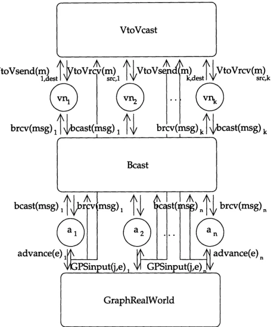
A physical node ai has an input GPSinput(loc)i from RealWorld, with loc E R3_{, which} func-tions as the aircraft's GPS oracle. A physical node ai also has an output action bcast(msg)i which outputs a message to Bcast, and brcv(msg)i which receives a message string msg from Bcast.

An output from ai, move(p, t)i to RealWorld also exists, which will be used to allow the soft-ware on a1 to control what occurs in RealWorld. The action will be used to control ai's

represen-tation in RealWorld, moving it to p within time t.

The remainder of the chapter is concerned with specifying the details of each component of the Network Layer, and putting them together as the formal definition for the Network Layer. I

Figure 3-1: Architecture of the Network Layer for I = {1, 2, ..., n}

begin each section with an overview of the component, including some motivation for decisions I make within. Then, formal definitions for each component are specified at the end of each

section.

3.2 Aircraft

-

The Physical Nodes

3.2.1 Overview

Aircraft serve as the physical nodes in our system. Each is equipped with a wireless commu-nication device with the ability to broadcast and receive messages. As they are aircraft, I must assume that their communication is reliable, and that spontaneous hardware failures happen very rarely. That said, one goal is to design a system that is able to recover from these failures

when they do happen.

While spontaneous failures are assumed to be rare, the network topology is constantly chang-ing. Since all the physical nodes are traveling, the set of physical nodes that any one physical node is in contact with may change dramatically between two points in time. Therefore, our

model must not rely on two specific physical nodes being in communication for any large pe-riod of time.

In addition to a communication device, our physical nodes have some computational power. In our simulations, a simple desktop computer has more than enough power to run the algo-rithms that we will be using. For the purposes of the model, though, we will formalize their computational abilities in terms of abstract machines.

Therefore, I formalize the physical nodes as timed input-output automata [19]. They have the ability to receive inputs, corresponding to the receipt of a message through the wireless net-work. They also have the ability to output, broadcasting their output over the wireless netnet-work. In addition, physical nodes have access to a GPS oracle, which provides each node with its own location information as it moves throughout space.

Aircraft also have an internal real-time clock, which we will assume to be synchronized with the clocks of other physical nodes in the system. The problem of clock synchronization is not trivial, and there is significant research into methods of clock synchronization over wireless net-works. That said, the use of a GPS service includes the use of an accurate clock for positioning, and since the algorithms in this thesis are not sensitive to small inconsistencies in time, for sim-plification we assume the aircrafts' clocks are synchronized.

3.2.2 Definitions

The type Msg is our finite message alphabet.

The set I represents the aircraft names that can be used to identify a unique aircraft.

For each i E I, ai represents a physical node in the Network Layer. The set of all such a₂ is called A. Each ai E A is a timed input-output automaton with the following actions:

* The output bcast(msg)i action outputs a message msg E Msg to Bcast. * The input brcv(msg)i action receives a message msg e Msg from Bcast. * The input GPSinput(loc)i action receives i's location loc E e 3 from RealWorld.

* The output move(p, t)i action to RealWorld, with t E R > 0 and p E R3_{, which will be used} to control i, moving it to p within time t.

For all messages msg E Msg output by as in a bcast(msg)i action, msg is a globally unique message. This can be achieved by requiring that all msg e Msg include a field for the sender of the message msg.sender = i and a field for the time of the message msg.time = now. The actual

message sent is simply msg.

In addition to these actions, ai may have other actions which must be internal, which are unspecified here.

The state of ai includes:

* now E R > 0, which is initialized to 0 and increases with rate 1.

Sloc R3 , which is updated on each GPSinput.

In addition to these variables, ai may have other state variables. Its transitions and trajecto-ries are unspecified, except as noted above.

3.3 Communications

-

The Bcast Service

3.3.1 Overview

As previously stated, the aircraft will be operating on a wireless ad-hoc network; there is no fixed infrastructure present to provide a reliable point of communication. A physical node on the net-work has only the ability to broadcast a message to all other physical nodes, of which some are able to receive the message, but those out of communications range neither receive the message nor any indication that they have missed a message. The physical nodes have no ability to send a message to a single desired recipient, nor determine what other physical nodes are in range.

I represent this communication network with the timed input-output automaton Bcast which receives messages from physical nodes and outputs those same messages to all physical nodes in communications range.

Communications Range

The range of a physical node's communications capability is fixed at a radius r, a distance in 3-space. No other physical nodes outside that range will receive broadcasts made by the

phys-ical node. Many complications arise from this assumption in a physphys-ical system that we, for the purposes of this model, can safely ignore, for these reasons:

* First, the communications range of different physical nodes will vary considerably based on the power of their transmitter. This is not a concern in this system, as we assume aircraft are all equipped with similar, standardized communications equipment.

* Second, the range may be affected by physical objects in the way, or interference from other equipment. Again, considering the space which we expect our network to be operat-ing in (thousands of feet above the ground), obstructions will not occur, and interference is prevented due to aircraft's use of dedicated frequencies for communication.

* Third, problems with signal strength arise in real systems, as some physical nodes may re-ceive corrupt or incomplete data at the edge of communication range. We assume that our assumed radius of communications r is such that within that range, anyone who receives a broadcast receives the complete message. While signal strength outside of the radius may vary, our algorithms will not depend on such messages, as you will see in the subsequent chapters.

Therefore, we are safe to assume that our broadcasts occur in a fiked radius r from the phys-ical node.

Communications Reliability and Delay

When a physical node broadcasts a message, all other physical nodes within range will receive the message, and all messages are received in the order which they are broadcast. While these may seem like bold claims or oversimplifications, they are justified ones.

On perfect reliability, this is a thesis about the abstraction of the Virtual Stationary Automa-ton and their use in developing an algorithm for free flight air traffic control. This is not in-tended to be a thesis about network reliability. There are many methods for performing com-munications reliability: our implementation of the VSA emulator uses an absolute ordering on messages along with rebroadcasts and state synchronization to ensure that each physical node within range receives all messages. This is not the only way to provide reliability, and an

imple-mentor may wish to choose a different one. Therefore, for the purposes of this thesis, I assume that the reliability problem has been solved at a lower level.

On perfect ordering, I turn back to our implementation of the VSA emulator [12, 13], which contains a built-in service to provide message ordering. There are a number of ways to imple-ment message ordering, and that is again, up to an impleimple-mentor and beyond the scope of this thesis.

I will not assume that messages are delivered instantaneously. Due to the rebroadcasts that may be required to ensure reliability and ordering, it may take a non-trivial amount of time to get a message from one physical node to another in range. That said, our bound on the reception range allows us to assume a high probability of delivery which we can use to define an upper bound on the message delay. We will call this bound d, and we can assume that any message broadcast by a physical node will reach all other physical nodes in range within that time d.

There are two reasons this system will support such a bound:

* While broadcasts may occur quite often, the upper bound on range allows us to assume retransmissions are rare. Therefore, we can assume that most of the time, the network is not saturated, and no physical node will be required to wait a long time to transmit. * There are no multiple-hop connections being made. Every message is a broadcast directly

from the sender of the message. As a broadcast can be made only when there are no trans-missions occurring already, the message will never be queued and will be delivered at the speed of the transmission medium immediately when sent.

Therefore, the claims of reliable message delivery and bounded transmission delay are jus-tified for the purposes of this thesis. While some of the justifications of the claims I have made are not fully explained at this point, they should be made clear as the algorithm is presented.

3.3.2 Definitions

A timed input-output automaton Bcast(d, r) represents the communications network in the Network Layer.

* d E R, the upper bound on message delay between inputting a message and outputting it to the appropriate physical nodes.

* r E R, the communications range.

For each i e I, Beast has the following actions:

* The input bcast(msg)i action, which receives a message msg E Msg from ai. * The output brcv(msg)i action, which sends a message msg E Msg to ai. * The input GPSinput(loc)i action receives i's location loc E R3 from RealWorld.

Beast contains a state variable locs, which is an array of locations, indexed by i E I, such that

locs[i] E R3 gets updated upon each GPSinput(loc)i action.

The behavior of Beast is as follows. Upon inputting bcast(msg)i from ai, within time d, Beast will output brcv(msg)j to each aj such that as and aj are within r distance of each other according to locs at the time the bcast was received by Beast. Note that this means a2 will always receive its

own broadcast.

Other requirements for the behavior of Beast include, for any three i, j, k e I where i, j, k

may or may not be equal:

* Message Ordering: If a bcast(msgl)i event precedes a bcast(msg2)j event, and if brcv(msgl)k and brcv(msg2)k both occur, then the brcv(msgl)k event precedes the brcv(msg2)k event. * Message Integrity: Each output brcv(msg)j must have been preceded by an input action

bcast(msg)i such that msg in the two actions is the same and the brcv(msg)j occurs at most d time after the bcast(msg)j action.

* Message Uniqueness: No two brcv(msg)i events occur for the same msg and the same i. In addition to these variables, Beast may have other state variables. Its transitions and tra-jectories are unspecified, except as noted above.

3.4 RealWorld

3.4.1 Overview

The physical world in the air traffic control system will be represented in the Network Layer by the timed input-output automaton RealWorld. The main goal of RealWorld is to keep track of the physical locations of the aircraft in the system, and to use that information to act as a GPS oracle to the physical nodes in A.

Airspace

The airspace for the air traffic control system is some contiguous subset of three-dimensional space. The airspace is represented by a connected deployment space R C R3. Aircraft are able to move freely in R, and we assume that they either never leave R, or if they do, then we are no longer concerned with them.

GPS Service

For each aircraft name i E I in the state of RealWorld, there is a corresponding physical node

ai E A for which RealWorld outputs periodic GPS updates. These updates are performed by the

output GPSinput(loc)i action, which is an input to both ai and Bcast.

These outputs are periodic with period e. The period E is chosen to be small enough that my algorithms can easily tolerate any slight inaccuracy in the location of aj. This is intended to closely resemble the behavior of real GPS devices, which update their location extremely fre-quently.

3.4.2 Definitions

The connected deployment space of the system is R C R3_.

A timed input-output automaton RealWorld(e, v_max) represents the physical state of the real world in the Physical Layer. The parameter e E R > 0 is the GPS update period, and is assumed to be small. The parameter vmax E R+ is the maximum velocity the aircraft can achieve.

Constants:

E , the GPS update frequency

ER >O

v_ max , the maximum aircraft velocity E R+

Signature:

Output GPSinput(loc)i , i E I, loc E R

Input move(p, t)i , p E R3, t E R > 0

InternalfinishMovej , i E I Internal Takeoff , i E I

Internal Landings , i E I

State:

GPSdone, an array of booleans for each i E I and for k E {0, 1, 2, 3...

initialized to false

aircraft, an array of type AircraftRecord for each aircraft[i], initialized to:

aircraft[i].loc +- loc- NULL aircraft[i].moving +- false aircraft[i].movingtime +- 0

aircraft [i].movingto +- loc- NULL

now: R

Trajectories: evolves

d(now) = 1

for each i E I, with a[i] = aircraft[i]:

if (a[i].loc= loc_-NULL) then

constant a[ i].loc else

0 < Id(a[i].loc)l < v-max

invariant

if (a[i].moving= true) then

dist(a[i].loc, a[i].movingto) < v_ max(a[i].movingtime - now)

stops when

any precondition is satisfied

Actions: Output GPSinput(loc)i Precondition: now= ke A GPSdone[i, k] = false A loc = aircraft[i].loc Effect: GPSdone[i, k] <- true

Input move(p, t)i

Effect:

if (dist(aircraft[i].loc, p) _ v_-max tA aircraft[i]. moving = false A

choose bE {true, false}) then

aircraft[i]. moving <- true

aircraft[i].movingtime +- now+ t

aircraft[i].movingto +- p

Internal finishMovei

Precondition:

aircraft[i].loc = aircraft[i].movingto A aircrafti]. moving = true

Effect:

aircrafti]. moving - false

Internal Takeoffs

Precondition:

now = aircraft[i]. t_- takeoffA aircraft i ].loc = loc_-NULL

Effect:

aircraft[i].loc - aircraft[i]. loc_- takeoff

Internal Landingi

Precondition:

aircraft[i]. loc = aircraft i ]. loc_- landing

Effect:

aircraft[i]. loc loc_-NULL

The constant location loc_ NULL e R3 _{- R is some location outside the deployment space}

which is used to initialize the location of aircraft before they enter the system. The data type AircraftRecord is a record with fields:

* t_takeoff E R > 0, the time the aircraft enters the system.

* loc_takeoff e R3, the location at which the aircraft enters the system.

* loc_landing E R3, the location at which the aircraft leaves the system.

* loc e R3_{, the current location of the aircraft.}

* moving, a boolean representing whether or not this aircraft is being controlled by a move

action.

* movingtime E R > 0, the deadline for finishing a move action.

* movingto E R, the location in R that the aircraft is moving to.

RealWorld also has a single output action, which is periodic with period E, as well as an input

action:

* The output GPSinput(loc)i action, where loc = aircraft[i].loc, and the output is received by

ai and Bcast. This output occurs for each i E I at now = 0, e, 2e, ....

* The input move(p, t)i action from ai, with t E R > 0 and p E R3_{, which will be used to} control i, moving it to p within time t. If a subsequent move(p', t')i occurs while the aircraft is moving, the subsequent action is ignored.

The path that i takes is nondeterministic, and nondeterministic flight resumes after reach-ing p. If the move action would force i to exceed the maximum velocity v_max, the action is ignored. The action can also be declared to be invalid nondeterministically.

The state of RealWorld includes:

* An array of AircraftRecords, aircraft, indexed by i E I. For each of these aircraft[il,

aircraft[i].t_takeoff, aircraft[i].loc_takeoff, aircraft[i].loc_landing are set in the initial

state of RealWorld. The values of aircraft[i].loctakeoff and aircraft[i].loc landing must be in R. The current location, aircraft[i].loc is initialized to loc_NULL.

The most important behavior of RealWorld is the motion of the aircraft. Upon initialization of the automaton, for each i E I, the value of aircraft[i].loc is set to the constant loc NULL.

At now = aircraft[i].ttakeoff an internal Takeoffi action occurs, and aircraft[i].loc's value

changes to aircraft [i].loc_ takeoff. The value of aircraft[i].loc then changes

nondeterministi-cally with a continuous, bounded derivative in R3, such that I d(aircrafti .lo < vmax.

Upon receiving a valid move(p, t)i action, aircraft[i].moving is set to true, aircraft [i].movingto

is set to p, and aircraft[i].movingtime is set to now + t. The aircraft i then moves to p within time

t, resuming its normal, nodeterministic movement after reaching p.

When aircraft[i].loc = aircraft[i].loc_landing, we consider i to have left the system, and an internal Landingi action occurs. This action changes aircraft[i].loc to loc_NULL and the trajectory which changes the value of aircraft[i].loc halts. The value of aircraft[i].loc does not change again.

3.5 The Physical Layer

I define the Physical Layer of our system, PLayer(R, E, vmax, d, r), depicted in Figure 3-1 at the

beginning of this chapter, to be the composition of these components: a single Bcast(d, r) TIOA, a single RealWorld(e, vmax) TIOA, and n physical node TIOAs which comprise the set A.

3.6 Chapter Summary

In this chapter I have:

* Enumerated the capabilities of the aircraft that will serve as physical nodes in our air traffic control system.

* Discussed the communications service Bcast, while making simplifying assumptions about its behavior.

* Described the RealWorld automaton, which models the physical state and motion of the world that the system operates in.

Chapter 4

The Continuous VSA Layer

The motivation behind the Continuous VSA Layer, or just the VSA Layer, is to use the volatile mobile network described in the previous section to simulate a number of virtual stationary automata, or VSAs, at various locations in space. We can think of these VSAs as virtual machines which are able to perform computations and store data, and are located in a stable location. Therefore, the VSA Layer provides us a stable platform for implementing applications that can rely on the locations of the VSAs.

In reality, of course, these VSAs are not present in the world, but instead they are emulated by a number of nearby physical nodes. This emulation is a protocol to ensure that the VSA remains active during both small and large changes in the network topology.

A number of previous models for the VSA have been previously developed. A theoretical in-depth treatment has been described in "Timed Virtual Stationary Automata for Mobile Net-works" [31, and more recently, a Python-based implementation has been described in "The Vir-tual Node Layer: A Programming Abstraction for Wireless Sensor Networks." [131. Other papers involving algorithms using the VSA also provide appropriate models for the VSA Layer [7, 8].

The VSA Layer will be specified in this chapter, including the architecture and the interac-tions of the layer. I will then describe some of the details of the VSA Layer's emulation, but this discussion will forgo some of the complex theoretical concerns of this emulation. Additional details of the emulation, if desired by the reader, can be found in Dolev, Gilbert, Lahiani, Lynch, and Nolte [3].

of each component of the VSA Layer, and putting them together as the formal definition for the VSA Layer. I begin each section with an overview of the component, including some motivation for decisions I make within. Then, formal definitions for each component are specified at the end of each section.

4.1 Regions

4.1.1 Overview

In order for the VSA Layer to work, the area that our network inhabits must be divided up into

regions. A single VSA is contained within each region. Each region also has a set of neighbors,

which are the nearby regions that the VSA in the region is able to communicate with.

The size of the regions and the set of neighbors for a region are chosen in order to satisfy the requirement that no matter where in a region a client is, its broadcast is able to reach every other client in the same region, and every other client in the region's neighbors. In general, this might mean that one region could be directly adjacent to another, yet not be considered a neighbor, if there are parts of the two regions that are not able to communicate with each other.

We choose the size and layout of the regions in our system to satisfy three requirements: 1. Each region's border is shared with another region (there are no regions that have a border

that does not have another region on the other side of it) unless that region is on the edge of the system.

2. Every region's neighbors are exactly the regions that share a border with it.

3. The maximal distance between any point in any region and any point in one of its neigh-bors is less than or equal to a communications range r parameter for the Continuous VSA Layer, CVLayer(d, r, E, v_max).

Adhering to these requirements will result in our space being partitioned into regions, within which a physical node is able to communicate with all other physical nodes in both its own region and neighboring regions.

4.1.2 Definitions

The parameter r E R+ is the communications range within the layer.

The set J represents the region names, as defined in the global constants of Section 2.5. The function region : R -- J maps a point in R to its region name. Each point in R has exactly one region name associated with it. A region is a subset S of R such that for some j e J,

S = {p e Rlregion(p) = j}. I assume that each region is connected.

The function inRegion : J, R3 _{-+ true, false is a predicate that returns true if a point in R}3 is in the appropriate region in J, and false otherwise. This function satisfies the condition that

region(p) = j +-+ inRegion(j,p) = true.

The function nbrs : J - 2J returns, on input j, the set of j's neighbors. It is required that for

all j, j' E J, ifj' E nbrs(j), then j E nbrs(j').

The following constraints are required for all regions j E J:

* Every region's neighbors are exactly the regions that share a border with it.

* For every point p such that region(p) = j, and all p' such that region(p') E {j} U nbrs(j),

p-p'

<I

r.

4.2 Architecture of the VSA Layer

The VSA Layer CVLayer(d, r, E, v_max) contains two sets of timed input-output automata[19]: the VSAs, fixed in a specific location in space, and the clients, which are mobile. Also, like the physical network layer, the VSA layer has a timed input-output automaton which represents the real world and another timed input-output automaton which represents broadcast communica-tions. In the VSA Layer, though, the broadcast communications automaton only allows a client to send messages to the VSA in its region, and receive messages from that same VSA. It does not allow for direct client-to-client communications. The VSA Layer also adds a timed input-output automaton to represent the communication between neighboring VSAs.

In many ways, the VSA layer looks similar to the network layer described in the previous chapter. The VSA layer includes the set A = {ai, a2, ..., an} of aircraft -timed input-output

rep-Figure 4-1: Architecture of the VSA Layer, for I = {1, 2, ..., n} and J = {1, 2, ..., k}

Client Automaton aj, for i E I Signature:

Input brcv(msg)i , msg Msg

Input GPSinput(loc)i , loc E R

Output bcast(msg)i , msg E Msg Output move(p, t)i , t E R>O, p E R State:

loc E R, the client's current location in space now : R, the current real time

2

4

6

8

10

resents the physical world that the aircraft operate in; and the timed input-output automaton

Bcast, which represents the broadcast medium for clients and VSAs.

In the VSA layer, we also have a set VN = {vnl, vn2, ..., vnk} of Virtual Stationary Automata, which are also timed input-output automata. In addition, a timed input-output automaton

VtoVcast represents the communications service between neighboring VSAs.

A client ai has an input GPSinput(loc)i from RealWorld which functions as the aircraft's GPS oracle. The input occurs periodically with some small period e.

A client a2 also has an output action bcast(msg)i which outputs a message to Beast, and

brcv(msg)i which receives a message from Bcast. The recipient of the message does not receive information on who the sender of the message was.

AVSA vnj has an output action bcast(msg)j which outputs a message to Bcast, and brcv(msg)j which receives a message from Bcast.

The VSA also has an output action VtoVsend(m)j,dest which outputs a message to VtoVcast with destination VSA vndest. Also, the VSA has an input action VtoVrcv(m)src,j which receives a message from VtoVcast from source VSA vn,,rc. Note that vndest and vnsrc must be neighbors of

vnj for VtoVcast to output these actions to their destination.

Figure 4-2: TIOA Signature for Clients and VSAs in the VSA Layer

Virtual Stationary Automaton vnj, for j E J Signature: Input brcv(msg)j , msg E Msg Input VtoVrcv(msg),,c,j , msg E Msg Output bcast(msg)j , msg E Msg Output VtoVsend(msg)j,dest , msg E Msg State:

now : R, the current real time

14

16 18

20

4.3 Clients

4.3.1 Overview

Clients are the mobile processes in the VSA Layer. They correspond very closely to the phys-ical nodes in the Network Layer, with similar capabilities and actions. A client can broadcast and receive messages, has access to a GPS oracle, and has an internal real-time clock which is synchronized with the other clients and Virtual Stationary Automata.

In the VSA Layer though, all outgoing messages from a client will be received only by a VSA. No messages are delivered to other clients. Conversely, a client only receives messages from a VSA, not from other clients.

4.3.2 Definitions

The set I represents the aircraft names that can be used to identify a unique aircraft.

For each i E I, in the VSA Layer ai represents a client. The set of all such ai is called A. Each

ai E A is a timed input-output automaton with the following actions:

* The output bcast(msg)i action outputs a message msg E Msg to Bcast. * The input brcv(msg)i action receives a message msg E Msg from Bcast. * The input GPSinput(loc)i action receives i's location loc E R3 from RealWorld.

* The output move(p, t)i action to RealWorld, with t E R > 0 and p E R , which will be used to control i, moving it to p within time t.

In addition to these actions, a2 may have other actions which must be internal, which are

unspecified here.

The state of ai includes:

* now E R > 0, which is initialized to 0 and increases with rate 1.

* loc E R3, which is updated on each GPSinput.

In addition to these variables, a2 may have other state variables. Its transitions and