Analytic redundancy and the design of robust failure detection systems

ANALYTICAL REDUNDANCY AND THE DESIGN OF ROBUST FAILURE DETECTION SYSTEMS

by

Edward Y. Chow Alan S. Willsky

This work was supported in part by the Office of Naval Research under Contract No. N00014-77-C-0224 and in part by NASA Ames Research Center under Grant No. NGL-22-009-124.

Analytical Redundancy

and

The Design of Robust Failure Detection Systems*

Edward Y. Chow (corresponding author) Schlumberger-Doll Research P. O. Box 307 Ridgefield, CT 06877 Tel. (203) 431-5419 and Alan S. Willsky

Laboratory for Information and Decision Systems Massachusetts Institute of Technology

Cambridge, MA 02139 Tel. (617) 253-2356

Abstract

The Failure Detection and Identification (FDI) process is viewed as consisting of two stages : residual generation and decision making. It is argued that a robust FDI system can be achieved by designing a robust residual generation process. Analytical redundancy, the basis for residual generation, is characterized in terms of a parity space. Using the concept of parity relations, residuals can be generated in a number of ways and the design of a robust residual generation process can be formulated as a minimax optimization problem. An example is included to illustrate this design methodology.

* This work was supported in part by the Office of Naval Research under Contract No. N00014-77-C-0224 and in part by NASA Ames Research Center under Grant No. NGL-22-009-124.

L INTRODUCTION

Physical systems are often subjected to unexpected changes, such as component failures and variations in operating condition, that tend to degrade overall system performance. We will refer to such changes as 'failures', although they may not represent the failing of physical components. In order to maintain a high level of performance, it is important that failures be promptly detected and identified so that appropriate remedies can be applied. Over the past decade numerous approaches to the problem of Failure Detection and Identification (FDI) in dynamical systems have been developed [1]; Detection Filters [2,31, the Generalized Likelihood Ratio (GLR) method [4,51, and the Multiple Model method [5,61 are some examples. All of these analytical methods require that a dynamic model of some sort be given. The goal of this paper is to investigate the issue of designing FDI systems which are robust to uncertainties in the models on which they are based.

The FDI process essentially consists of two stages: residual generation and decision making. For a particular set of hypothesized failures, a FDI system has the structure shown in Figure 1. Outputs from sensors are initially processed to enhance the effect of a failure (if present) so that it can be recognized. The processed measurements are called the residuals, and the enhanced failure effect on the residuals is called the signature of the failure. Intuitively, the residuals represent the difference between various functions of the observed sensor outputs and the expected values of these functions in the normal (no-fail) mode. In the absence of a failure residuals should be unbiased, showing agreement between observed and expected normal behavior of the system; a failure signature typically takes the form of residual biases

that are characteristic of the failure. Thus, residual generation is based on knowledge of the normal behavior of the system. The actual process of residual generation can vary in complexity. For example, in voting systems [7,8] the residuals are simply the differences of the outputs of the various like sensors, whereas in a GLR system, the residuals are the innovations generated by the Kalman filter.

In. the second stage of an FDI algorithm, the decision process, the residuals are examined for the presence of failure signatures. Decision functions or statistics are calculated using the residuals, and a decision rule is then applied to the decision statistics to determine if any failure has occurred. A decision process may consist of a simple threshold test on the instantaneous values or moving averages of the residuals, or it may be based directly on methods of statistical decision theory, e.g. the Sequential Probability Ratio Test [9].

The first concern in the design of an FDI system is detection performance, i.e. the ability to detect and identify failures promptly and correctly with minimal delays and false alarms. In the literature, this issue has typically been dealt with using a given model of the normal system behavior. An equally important design issue that is necessarily examined in practice but has received little theoretical attention is robustness: minimizing the sensitivity of detection performance to model errors and uncertainties. An ideal simplistic approach to designing a robust FDI system is to include all uncertainties in the overall problem specification; then a robust design is obtained by optimizing (in some sense) the performance of the entire system with the uncertainties present. However, this generally leads to a complex mathematical problem that is too difficult to solve in practice. On the other hand, a simple approach

is to ignore all model uncertainties in the performance optimization process. The

resulting design is then evaluated in the presence of modelling errors. If the

degradation in performance is tolerable, the design is accepted. Otherwise, it is

modified and re-evaluated. Although this method often yields acceptable designs, it

has several drawbacks. For example, it may be unclear what parts of the design

should be modified and what form the modification should take. Furthermore, each

iteration may be very expensive to carry out since extensive Monte Carlo simulations

are often required for performance evaluations.

In this paper we develop a systematic approach that considers uncertainties directly.

Our work is motivated by the practical design effort of Deckert, et. al. for an aircraft

sensor FDI system [10]. The basic idea used in this work was to identify the

analytical redundancy relations of the system that were known well and those that

contained substantial uncertainties.

An FDI system (i.e. its residual generation

process) was then designed based primarily on the well-known relationships (and only

secondarily on the less well-known relations) of the system behavior. As model error

directly affect residual generation, this approach suggests that robustness can be

effectively achieved by designing a robust residual generation process. In our work,

we have extracted and extended the practical idea underlying this application and

developed a general approach to the design of robust FDI algorithm. In addition to its

use in specifying residual generation procedure, our approach is also useful as it can

provide a quantitative measure of the attainable level of robustness in the early stages

of a design. This can allow the designer to assess what he can expect in terms of

overall performance.

In order to develop residual generation procedures, it is important to identify the

redundancy relations of a system and to characterize them according to how they are

affected by model errors and uncertainties. In this paper, we further develop the

concept of analytical redundancy that is used in [10,11], and we use this as a basis for

determining redundancy relations to be used for residual generation which are least

sensitive to model errors.

In Section II we describe the concept of analytical redundancy and present a

mathematical characterization of redundancy in linear dynamical systems that extends

ideas developed previously. We also provide for the first time a clear, general

interpretation of a redundancy relation as a reduced-order

Auto-Regressive-Moving-Average (ARMA) model and use this in Section III to describe the various ways that

analytical redundancy can be used for residual generation and FDI. In Section IV a

method of determining redundancy relations that are least sensitive to model error

and noise effects is described.

A numerical example illustrating some of the

developed concepts is presented in Section V. Conclusions and discussions are

included in Section VI.

IL ANALYTICAL REDUNDANCY - PARITY RELATIONS

The basis for residual generation is analytical redundancy, which essentially takes two forms : 1) direct redundancy - the relationship among instantaneous outputs of sensors, and 2) temporal redundancy - the relationship among the histories of sensor

outputs and actuator inputs. It is based on these relationships that outputs of (dissimilar) sensors (at different times) can be compared. The residuals resulting from these comparisons are then measures of the discrepancy between the behavior of observed sensor outputs and the behavior that should result under normal conditions. Examples where direct redundancy was exploited include [7,8,11,12,13]; explicit use of temporal redundancy was made in [101.

In order to develop a clear picture of redundancy, consider the following deterministic model:

x(k+1) - A x(k) + ~ bj uj(k)

j-l (la)

yj(k) - cj x(k),

j - 1,..., M

(Ib) where x is the N-dimensional state vector, A is a constant N x N matrix, bj is a constant column N-vector, and cj is a constant row N-vector. The scalar uj is the

known input to the j-th actuator, and the scalar yj is the output of the j-th sensor.

Direct redundancy exists among sensors whose outputs are algebraically related, i.e. the sensor outputs are related in such a way that the variable one sensor measures can be determined by the instantaneous outputs of the other sensors. For the system (1), this corresponds to the situation where a number of the cj's are linearly

dependent. In this case, the value of one of the observations can be written as a linear combination of the other outputs. For example, we might have

M

y

1

(k)

- ai yi (k)

i-2 (2)

where the ai's are constants. This indicates that under normal conditions the the ideal output of sensor 1 can be calculated from those of the remaining sensors. In the

absence of a failure in the sensors, the residual, YI (k)- aiyi(k) should be zero. A i-2

deviation form this behavior provides the indication that one of the sensors has failed. This is the underlying principle used in Strapdown Inertial Reference Unit (SIRU) FDI [7,8]. Note that while direct redundancy is useful for sensor failure detection it is not useful for detecting actuator failures (as modelled by a change in the bj, for instance).

Because temporal redundancy relates sensor output and actuator inputs, it can potentially be used for both sensor and actuator FDI. For example, consider the relationship between velocity (v) and acceleration (a):

v(k+l) - v(k) + Ta(k)

(3)

where T is the sampling interval. Equation (3) prescribes a way of comparing velocity measurements and accelerometer outputs (by checking to see if the residual, v(k+ 1)-v(k)-Ta(k),is zero) that may be used in a mixed velocity-acceleration sensor voting system for the detection of both types of sensor failures. Temporal redundancy facilitates the comparison of sensors among which direct redundancy does not exist. Hence it can lead to a reduction of hardware redundancy for sensor FDI. Viewed in a

can in principle be detected with the same level of hardware redundancy.

To see how temporal redundancy can be exploited for detecting actuator failures,

let us consider a simplified first-order model of a vehicle in motion:

v(k+l) -

av(k)

+ Tu(k)

(4)

where v denotes the vehicle's velocity, a is a scalar constant between zero and one

reflecting the effect of friction and drag. T is the sampling interval, and u is the

commanded engine force (actuator input) divided by the vehicle's mass. Now the

velocity measurements can be compared to the actuator inputs by means of (4), i.e.

through examining the residual v(k+l)-av(k)-Tu(k). An actuator failure can be

inferred, if the sensor is functioning normally but the residual is nonzero.

While the additional information supplied by dissimilar sensors and actuators at

different times through temporal redundancy facilitates the detection of a greater

variety of failures and reduces hardware redundancy, exploitation of this additional

information often results in increased computational complexity, since the dynamics of

the system are used in the residual generation process. However, the major issue in

the use of analytical redundancy is the inevitable uncertainty in our knowledge of the

system dynamics (e.g. of a in (4)) and the consequences of the this uncertainty on

the robustness of the resulting FDI algorithm. From the above discussion one

approach to the design of robust residual generation in any given application is

evident: first, the various redundancies that are relevant to the failures under

consideration are to be determined; then, residual generation is based on those

relations that are least sensitive to parameter uncertainties. This is the approach we

have adopted. In the remainder of this section we will present a characterization of

analytical redundancy and in a subsequent section we will quantify the effect of

uncertainties on a redundancy relation.

The Generalized Parity Space

Let us define

Cj

cjA I

ciAk

The well-known Cayley-Hamilton theorem [14] implies that there is an nj, 1lnjSN,

such that

, k+l

k<nj

rank C (k)

-

| n1

k< nj

(6)

The null space of the matrix Cj(nj-1) is known as the unobservable subspace of the

j-th sensor. The rows of Cj(nj-1) spans a subspace of RN that is the orthogonal

complement of the unobservable subspace. Such a subspace will be referred to as the

observable subspace of the j-th sensor, and it has dimension nj.

N

Let o be a row vector of dimension n-:(ni+l) such that -[o

1,

...

oM],

i-I

where j _{, j=-1,...,M, is a (nj+l)-dimensional row vector. Consider a nonzero o}

Cl (nl)

(7)

CM (nM

)

_,

Note that in the above equation Cj(nj) has nj+l rows while it is only of rank nj. The

reason for this will become clear when we discuss the temporal redundancy for a

single sensor. Assuming that the system (1) is observable, there are only n-N linearly

independent io's satisfying (7). We let Qf be an (n-N)xN matrix with a set of such

independent <o's as its rows. (The matrix fl is not unique.) Assuming all the inputs

are zero for the moment, we have

Yl (k,nl)

P(k)-

n

(8)

iYM (k,nM)

I

where

r

yj(k)

1

Yj (k,nj) -

, i 1...

M

1

_{yj (k+nj)}

Note that Equation (8) is independent of the state x(k). The (n-N)-vector P(k) is

called the

parity

vector. In the absence of noise and failures, P(k)=O. In the noisy

no-fail case, P(k) is a zero-mean random vector. Under noise and failures, P(k) will

become biased. Moreover, different failures will produce different (biases in the)

P(k)'s. Thus, the parity vector may be used as the signature-carrying residual for

III.

When the actuator inputs are not zero, (8) must be modified to take into account

this effect. In this case

YI (k,nl)

1

[B(n)

P(k) -

.

U (k,n

}

o) IYM (k,n) IBM (nM)

I

where

0 0 ....

0

cjB 0 ~ cjB · . B (nj)

-

. cjAnJ-'B cjAnJ-2_{B . . cjB 0 0} B -[bl,.., bq] u(k) -

[u

1(k),..., uq(k)]' no - max(nl, . . . , nM)

U(k, n) - [u'(k),..., u'(k+no)]'

(9) only involves the measurable inputs and outputs of the system, and it does not depend on the state x(k) which is not directly measured.

The quantity P(k) is known as the generalized parity vector, which is nonzero (or non-zero mean if noise is present) only if a failure is present. The (n-N) dimensional space of all such vectors is called the generalized parity space. Under the no-fail situation (P(k)=0), (9) characterizes all the analytical redundancies for the system (1), because it specifies all the possible relationships among the actuator inputs and sensor outputs. Any linear combination of the rows of (9) is called a parity equation or

a parity relation; any linear combination of the right-hand side of (9)'is called a parity function. Equation (6) implies that we do not need to consider a higher dimensional

parity space that is defined by (9) with nj replaced by lj> nj, j=1,...,M, although it is possible to do so. We note that the generalized parity space we have just defined here is an extension of the parity space considered by Potter and Suman [11] to include sensor outputs and actuator inputs at different times. In [11], Potter and Suman studied exclusively (9) with nl-n 2- ... 0.

A useful notion in describing analytical redundancy is the order of a redundancy relation. Consider a parity relation (under the no-fail condition) defined by

M

,, [Yj(k,nj) - Bj(nj) U(k,n)] - 0

i-I (1 0)

We can define the order p of such a relation as follows. Since some of the elements of a may be zero, there is a largest index Ai such that the fi-th element of xi _{for some}

i is nonzero but the C(+l)-st through the (nj+1)-st elements of each w are zero. Then p is defined to be fi-1. The order p describes the "memory span' of the

redundancy relation. For example, when p-O, instantaneous outputs of sensors are

involved. When p>O, a time window of size p+l of sensor outputs and actuator

inputs are considered in the parity equation. For example, (3) is a first order parity

relation.

To provide more insights into the nature of parity relations, it is useful to examine

several examples.

1. Direct Redundancy

Suppose there are J's of the form

- [o1,~,0,..., 01

where at least two of the w4's are nonzero, and they satisfy Equation (7). Then we

have the following direct redundancy relation

yl (k)

l

I

o, . -. M]

o

jyM (k)

Note that the above expression represents a zeroth order parity equation.

2. A Single Sensor

Equation (6) implies that it is always possible to find a nonzero x such that

) [Yj (k,nj) - Bj (n)U (k,n0)] -

0

(11)

Note that Equation (11) is of order nj, and it is a special case of (10). (This is why

we have used nj instead of nj-l in (7) in order to include this type of temporal

redundancy.) Since this redundancy relation involves only one sensor the parity

function defined by the left-hand side of (11) may be used as the residual for a

self-test for sensor j, if Bj(n) -0 or if the actuators can be verified (by other

means) to be functioning properly. Similarly, it can be used to detect actuator

failures if sensor j can be verified to be normal. Equation (4) (in which v(k) is

directly measured) represents an example of this type.

Alternatively (11) can be re-written as

It-i t-l

1

(12)

yj (k) -- ) l i

st

yj(k-t)- - odjj-t u(k-t)

where

d..,

* * *, C-1 0,..., 01] .BJjIj)

-i, t0O,...,nj-1, is a q-dimensional row vector, and ao, t-0,...,nj-1 is the (t+ 1)-st

component of w. Equation (12) represents a reduced-order ARMA model for the

j-th sensor alone. That is to say, the output of sensor j can be predicted from its

past outputs and past actuator inputs according to (12). Based on the ARMA

model several methods of residual generation are possible. We will discuss this

further in Section III.

3. Temporal Redundancy Between Two Sensors

A temporal redundancy exists between sensor i and sensor j if there are

si t ho r

O]

s tere... elJ-to0]

'Yi(k l n ) _{BBi (k,ni) (13)}

0 Yj (k,nj) -Bj(k~fj)

U(kno)

0

I~~~~~

1

)~~~~~~(13)

Equation (13) is a special case of the general form of parity equation (10) in the no-fail situation with os- 0 for s;i, s;j. The relation (13) is of order

p<max(ni,nj). Clearly, (13) holds if and only if

LO (dilICi(ni-l) ... ,- s , jlcj(nj-1)

(14)

and, (14) implies that a redundancy relation exists between two sensors if their observable subspaces overlap. Furthermore, when the overlap subspace is of dimension i, there are ii linearly independent vectors of the form [oi,w] that will satisfy (13). Note that (3) (with both v(k) and a(k) measured) represents an example of this type.

Because the order of (13) is p, either %, or o' must be nonzero. Assuming O •0, we can re-write (14) in an ARMA representation for sensor j as in (12)

yfk)-

-(w)l I

6Jyj(k-t) +

i

optYi(k-t) - i (opit+0po t)u(k-

t)

t-I t-O t-O

That is, the parity relation (13) specifies an ARMA model for the jth sensor, with the original system input u and the ith sensor output acting as inputs to this reduced order model. In general, any parity relation specifies an ARMA model for some sensor driven by u and by possibly all of the other sensor outputs.

III. RESIDUAL GENERATION FOR FDI

In the first part of this section we discuss alternative residual generation

procedures, and in the latter half of the section we discuss how such residuals, once

generated, can be used for failure detection. Our development in this section section

will be carried out in terms of a second order system (N =2) in the form of (1) with

the following parameters.

[all al:]

A b

0

a

22

b

(15)

C!-

[1

01

c

2

-

[0

1]

In this case nl-2, n

2-1,

and n-N-3. Therefore, there are only three linearly

independent parity equations which may be written as

Y1 (k)

-

(all +a

2

2)Y

1

(k- )

+ alla22

yl (k-2)

- a 2u (k-2) -

0

yj (k)- a, yl(k-1)- a2

Y2

(k-1) - 0

(16)

y

2

(k) - a

22

y

2

(k-1) - u(k-1) - 0

Note that these represent temporal redundancies.

Residual Generation Based on Parity Relations

For a zeroth order parity relation (i.e. a direct redundancy relation) the residual is

the corresponding parity function. For a higher order parity relation (temporal

redundancy), there are three possible methods for the residual generation. We will

illustrate these using the second parity equation of (16).

1. Parity Function as Residuals

Just as with direct redundancy relations, the parity function itself can be taken as a residual. For our specific example, this would be

rl(k) - yl(k)-allyl (k-1)-a 12Y2(k-l)

(17)

Such a residual is a moving average process, i.e. it is a function of a sliding window of the most recent sensor output and (possibly) actuator input values. It is useful to note the effect of noise and failures on the residual. Specifically, if the sensor outputs are corrupted by white noise, the parity function values will be correlated over the length of the window. In our example, rl(k) is correlated with rl (k-l) and rl (k+l) but not with any of its values removed by more than one time step .

The effect of a failure on a parity function depends, of course, on the nature of the failure. To illustrate what typically occurs, consider the case in which one sensor develops a bias. Since the parity function is a moving average process it also develops a bias, taking at most p steps to reach the steady state value. In our example, if y2(k) develops a bias of size

f

at time 0, rI (k) will have a bias of size

-a 12 6 from time 0+1 on.

2. Open-Loop Residuals

As discussed in the preceding section, any temporal redundancy relation specifies an ARMA model. In our example we have the model

yl(k) -all yl (k-1) +a 12y 2(k-1)

(18) This equation leads naturally to a second residual generation procedure: solve equation (18) recursively using as initial condition the actual initial value of the

recursion; compare the result at each instant of time to the actual output of sensor 1. That is, we compute

:Y (k) -all :l (k- 1) +a 12 Y2 (k-l)

(19) with

1 (0) - y1(0)

and the resulting residual is

r2(k) y (k)

-The behavior of this residual is decidedly different from that of rl (k). In particular, r2(k) is not a moving average of previous values as it involves the

integration of y2 (k). Thus, if yl(k) and y2(k) are corrupted by white noise, r2(k)

will in general be correlated with all of its preceeding and future values. For

example, if all-1, r

2

(k) is nothing but a random walk.

The effect of failure is also different in r2(k). For example, if y2(k) develops a

bias, this bias will be integrated in (19). In particular, if all_-1, r2(k) will develop

a ramp of slope -ale2 at time time 0+1 if sensor 2 develops a bias of size 6 at time 9.

3. Closed-Loop Residuals

A third method of residual generation is also based on the ARMA model (18), but explicitly taking noise into account. Specifically, we write each sensor output as its noise free value plus noise:

Yi (k) - yi, (k) + vi (k)

(20)

Then, from (18) we obtain the equation

ylo(k) - allylo(k-1) + al₂y₂(k-1) - al₂v₂(k-1)

(21)

Note that the known driving term here is the actual sensor output, and thus the noise on this output becomes a driving noise for the model (21). Given this model and the noisy measurement Yl (k) of ylo(k) we can design a Kalman filter

Y

10o(k) - all o(k-1) + al0 2y2(k-1) + H r3(k)

where H is the Kalman gain and the residual is the innovations

r3(k) - yl(k) - atl~l (k-1) - al2y2(k-l)

In this case, r3(k) is an uncorrelated sequence. Also, if Y2(k) develops a bias at

time 9, the trend in r3(k) will be time-varying. Specifically, it will begin at time

0+1 as a ramp, but will level off to a steady state bias due to the closed-loop nature of the the residual generation process.

All three of these residual generation procedures have been used in practice. For example, parity functions have found many applications, ranging from gyro failure detection [7,8] to the validation of signals in nuclear plants [13]. The open-loop method was used in detecting sensor failures on the F-8 aircraft [101, as was the closed-loop method, which has also been used in such applications as electrocardiogram analysis [6] and manuever detection [151. Our contribution here is to expose the fundamental relationships among these in general.

At first glance, it might seem that the closed-loop method is the logical method to use in that, if the sensor noise is white, it produces an uncorrelated sequence of residuals rather than a correlated one that would have to be whitened in an 'optimal' detection system. In fact, going one step further, it would seem decidedly suboptimal

to use only one or several redundancy relations rather than all of them. That is, the 'optimal' approach would seem to be designing a Kalman filter based on the entire model (1). This, however, is true only in the most ideal of worlds in which our knowledge of the system dynamics is perfect. When model uncertainties are taken into account it is not at all clear that this is what one should do. Rather, it would seem reasonable to identify only the most robust redundancy relations and then to structure failure detection systems based on these. This leads to two obvious questions:

1. How does one define and determine robust redundancy relations ?

2. Given a set of such relations, how does one use them in concert in designing a failure detection system ?

In the remainder of this section we discuss the second of these questions, while the first is addressed in the next section. Throughout these developments we will focus on using the first (i.e. the parity function) method of residual generation, as this is the simplest analytically while allowing us to gain considerable insight and develop some very useful techniques for robust failure detection.

Use of Parity Functions in a Failure Detection System

failure detection. In this discussion we will not be concerned with the detailed

decision process, which would involve specific statistical tests, but we will focus on the

geometry of the failure detection problem. First we will examine (sensor) FDI using

direct redundancy. This is the case that has been examined in most detail in the

literature, for example, in the work of Evans and Wilcox [7], Gilmore and McKern

[8], Potter and Suman [11], Daley, et. al. [12], and Desai and Ray [13]. We include

this brief discussion of concepts developed by others in order to provide for a basis for

our discussion of their extention to include temporal redundancy relations.

Consider a set of M sensors with output vector y(k) - [yl (k),...,yM (k) ' and a parity

vector

Pk) (k) - y()

(22)

where Qi is a matrix with M columns and a number of rows (the specification of

which will be discussed later). From Section II, we see that fl is not unique, and for

any choice of fl such that (22) is a parity vector, we know that P(k) will be zero in

the absence of a failure (and no noise). However, the nature of failure signatures

contained in the parity vector depends heavily on the choice of fi. Clearly f should

be chosen so that failure signatures are easily recognizable. In the following we will

describe two approaches for achieving this purpose.

One way of using the parity vector for FDI is via what we term a voting scheme. To

implement the voting scheme, we need a set of parity relations such that each

component (i.e. sensor or actuator) of interest is included in at least one parity

relation and each component is excluded from at least one parity relation. When a

component fails, all the parity relations involving it will be violatedl, while those

excluding it will still hold. This means that the components involved in parity

relations that hold can be immediately declared as unfailed, while the component that

is common to all violated parity relations is readily identified as failed. This is the

basic idea of voting that is used in [7,8]. In fact, for the detection and identification

of a single failure among M components at least M-1 parity relations are required

2

_.

Therefore, the number of rows in /1 should be at least M-1, and the rows of /1

should be chosen to satisfy the above criterion on the set of parity relations.

Furthermore, we note that at least three components are needed for voting and that it

may not be possible to determine a required /f in many applications, in which case

the use of temporal redundancy is absolutely necessary.

Another method which uses more information about how failures affect the

residuals has been examined by Potter and Suman [111, and Daley, et. al. [I1]. This

method exploits the following phenomenon.

A faulty sensor, say the j-th one,

contains an error signal v (k) in its output

yj(k) - C x(k) + v (k)

(23)

The effect of this failure on the parity vector defined by (22) is

P(k) -

lj

Y (k)

where Qij is the j-th column of Qf.

That is, no matter what v (k) is, the effect of a

1. 'Violation' can be defined in a variety of ways. Typically, one compares the residual value to a threshold determined by some means (e.g. one may use a statistical criterion to set the threshold to achieve a specified false alarm- correct detection tradeoff). Alternatively, one may use the average of the residual over a sliding window to improve the tradeoff.

2. The logic used here has to be modified slightly. If each of the M-1 components is excluded from a different parity relation and the remaining component is involved in all parity relations, then violation of all parity relations indicates the failure of this last component, and failures in the other components can be identified using the above logic. In practice, more than M-1 relations are preferred for better performance in noise.

sensor j failure on the residual always lies in the direction 1lj. Thus, a sensor j failure

can be identified by recognizing a residual bias in the flj direction. We refer to 1fj is

the Failure Direction in Parity Space (FDPS) corresponding to sensor j. (In [11] fli is

referred to as the j-th measurement axis in parity space.)

It is now clear that fi should be chosen to have distinct columns, so that a sensor

failure can be inferred from the presence of a residual bias in its corresponding FDPS.

(Note that an fl suitable for the voting scheme has M distinct columns.) In principle,

an fi with as few as two rows but M distinct columns is sufficient for detecting and

identifying a failure among the M sensors. In practice, however, increasing the row

dimension of SI can help to separate the various FDPS's and increase the

distinguishability of the different failures under noisy conditions.

The two FDI methods discussed above can also be used with temporal redundancy.

In a voting scheme, one can see that the same logic applies. (In fact, additional

self-tests may be performed for the sensors providing corroboratory information which is

of great value when noise is present.) Consider next the extention of the second

failure detection method to temporal redundancy relations. In this case, it is generally

not possible to find an fQ to confine the effect of each component failure to a fixed

direction in parity space. To see this, consider the parity relations (16). We can write

the parity vector as

yI

(k)

fI

-(all+a

22

) alla

2 2

0

0 | y

1

(k-

1)

-a12i(k)

P(k) - -a _{1 2} 0 0 -a ₁₂ Yl(k-2) +

10

0

1

(k-2)

o

0

0

1 -a

22

Iy

2

(k)

1 0

When sensor 2 fails (with output model (23)), the residual vector develops a bias of

the form

P(k) -

v(k)

+ -al2

v(k-l)

1.

I-a22 l(24)

Unless v (k) is a constant, the effect (signature) of a sensor 2 failure is only confined

to a two-dimensional subspace of the parity space. In fact, generally when temporal

redundancy is used in the parity function method for residual generation, failure

signatures are generally constrained to multi-dimensional subspace in the parity space.

These subspaces may in general overlap with one another, or some may be contained

in others. If no such subspace is contained in another, identification of the failure is

still possible by determining which subspace the residual bias lies in. We note that the

detection filters of Beard [21 and Jones [31 effectively acts, in a closed-loop fashion, to

confine the signature of an actuator failure to a single direction and that of a sensor

failure to a two-dimensional subspace in the residual space.

As we indicated previouly, the second approach to using parity functions for FDI

uses some information about the nature of the failure signatures. Specifically, it uses

information concerning the subspaces in which the signatures evolve. In this approach

no attempt is made to use any information concerning the temporal structure of this

evolution. (For example, no assumption was made about the evolution of v(k) in

(24).) In some problems (e.g. in [6,101) one may be able to model the evolution of

failures as a function of time. In this case, the temporal signature of the failure (in

addition to the subspace information discussed above) can be determined. (If, for

instance, v (k) in (23) is modelled in a particular way, then one immediately obtains a

·model of the evolution of P(k) in (24).) Such information can be of further help in

distinguishing the various failures, especially in the case where temporal redundancy is

used. Detection systems such as GLR [4,5,6] heavily exploit such information

contained in the residual.

IV. PARITY RELATIONS FOR ROBUST RESIDUAL GENERATION

In this section we discuss the issue of robust failure detection in terms of the

notions introduced in the previous section. The need for this development comes

from the obvious fact that in any application a deterministic model such as (1) is quite

idealistic. In particular, the true system will be subjected to noise and parameter

uncertainty. If noise alone were present one could take this into account, as we have

indicated, through the design of a statistical test based on the generated residuals (see,

for example, [4,101). However, the question of developing a methodology for FDI

that also takes parameter uncertainty into account has not been treated in the

literature previouly. It is this problem we address here.

The starting point of our development is a model that has the same form as (1)

but includes noise disturbance and parameter uncertainty:

x(k+l) - A 7( ) x(k) + bj(,) uj(k) + (k)

i- l(25a)

yj (k) - cj x (k) + 7-j (k)

(25b)

where y is the vector of uncertain parameters taking values in a specified subset

r

of

R

m

. This form allows the modelling of elements in the system matrices as uncertain

quantities that may be functions of a common quantity.

The vectors 5 and

X a[l,.. ',* 7M]' are independent, zero-mean, white Gaussian noise vectors with

constant covariance matrices Q ( 0) and R((>0) respectively.

In this section we

consider the problem of determining useful parity relations that can be used for FDI

for the system described by (25).

The Structure and Coefficients of a Parity Function

Before we continue with the discussion, it is useful to define the structure and the

coefficients of a parity function. Recall that a parity function is essentially a weighted

combination of a (time) window of sensor outputs and actuator inputs. The structure

of a parity function defines which input and output elements are included in this

window, and the coefficients are the (nonzero) weights corresponding to these

elements. A scalar parity function, p(k), can be written as

p(k) - aY (k) + /3U (k)

(26)

where Y(k) and U (k) denote the vectors containing the output and input elements in

the parity function, respectively. Together, Y (k) and U (k) specify the parity

structure, and the row vectors a and , contain the parity coefficients. Consider, for

example, the first parity function of (16).

Its corresponding Y(k), U(k),

a,

and /8

are

Y(k) - [yl(k-2), yl(k-1), yl(k)

1'

U (k)- u(k-2)

a -[alla _{2 2}, -(all+a 22 ), 1]

-- -a 12

Under model (25), Y (k) has the form

Y (k) - c(y) x(k-p) + < (y) (k) + B (y) U (k) + ~ (k)

where p is the order of the parity function, and

j(k) - [~'(k-p),..., f'(k-1)]'

The components of j(k) and U(k), and the rows of C(y), D(y7), and B are

determined from (25) and the structure of Y (k). If, specifically, the i-th component

of Y (k) is ys(k- o), then the i-th component of

i

(k) is

i

(k)

-?

(k-a)

The vectors

4

and ii are independent zero-mean Gaussian random sequences with

constant covariances Q and R, respectively. The matrix Q is block diagonal with Q on

the diagonal; Rij-Rsta, where Rij is the (ij)-th element of R, S,. is the Kronecker

delta function, Rts is the (s,t)-th element of R, and the ith element of Y(k) is

y (k-a.), while the jth element is yt(k-'). The i-th row of C(y), i.e. C(i,y) is

C (i,y) - csAP

-The i-th row, )(i,y), of 1/(y) (which has pN columns) is

(i,y) - [csAp-'- 1, csAP- '-2, . . ., c, 0,..., 0]

Note that x(k-p) is a random vector that is uncorrelated with

Z

and e, and EJ x(k-p)I - xo(k-p)

covx (k-p) - Z(y)

where I(y) is the (steady state) covariance of x (k-p) and it is dependent on y through A(y) and B(y).

matrix B all the rows in Bj(k,y) (see Equation (9)) corresponding to C(i,y). Then,

collect all the non-zero columns of B into B and the corresponding components of u

in the window into U(k).

In the preceeding section, we defined parity functions as linear combinations of

inputs and outputs that would be identically zero in the absence of noise. When

parameter uncertainties are included, however, it is not possible in general to find any

parity functions in this narrow sense. In particular, with reference to the function

p(k) defined by (26) and (27) this condition would require that aC(y) -0 for all

y

c

r.

Consequently, we must modify our notion of a useful parity relation.

Intuitively, any given parity structure will be useful for failure detection if we can find

a set of parity coefficients that will make the resulting function p(k) in (26) close

.to

zero for all values of

ycr

when no failure has occurred. When considering the use

of such a function for the detection of a particular failure one would also want to

guaranty that p(k) deviates significantly from zero for all y C

r

when this failure

occurs. Such a parity structure-coefficient combination approximates the true parity

function defined in Section II. Our approach to the robustness issue is founded on

this perspective of the FDI design problem, and we will choose parity structures and

coefficients that display these properties. From this vantage point, it is not neccessary

to base a parity structure on a C with linearly dependent rows. Of course, the closer

the rows of C are to being dependent the less the value of the state x(k-p) will affect

the value of the approximate parity function, i.e. the the closer the approximate parity

function is to being a true parity function.

Clearly, there are many candidate parity structures for a given system. For a voting system, the requirements on SI as described in Section HI help to limit the number of such candidates that must be considered. In addition special features of the system under consideration typically provide additional insights into the choice of candidate parity structures. Given the set of candidate structures one is faced with the problem of finding the best coefficients for each and then with comparing the resulting candidates. In this paper we will not address the problem of defining the set of candidate structures (as this is very much a system-specific question) but will assume that we have such a set of structures*, and we will proceed to consider the problem of determining the coefficients for these structures and their comparison. In the following we will describe a method for choosing robust parity functions. Although this approach represents only one method of solving the problem, it serves well to illustrate the basic ideas of a useful design methodology.

The parity function design problem is approached in two steps: 1) coefficients that will make the candidate parity functions close to zero under the no-fail situation are determined, 2) the resulting parity functions that provide the most prominant failure signatures for a specified failure will be chosen. We will consider the coefficient design problem first.

We are concerned with the choice of the coefficients, a and ,8 for the parity function

p(k) - a [C(y) x(k-p) + $(y) '(k) + B(y) U(k) +

j(k)

- 8U(k)

Note the dependence of p(k) on a, ,8, y, x(k-p), and U(k). As p(k) is a random * This set could be all structures up to a specified order, which is a finite set.

variable, a convenient measure of the magnitude (squared) of p(k) is its variance, El p2(k) , where the expectation is taken with respect to the joint probability density of x(k-p), a(k), and j(k) with the mean xo(k-p) and the value of U(k) assumed known. As we will discuss shortly, this can be thought of as specifying a particular operating condition for the system. Note also that the statistics of x(k-p) depend on y. Define

e(a,,8) - max El p2_(k)

ycr

(28)

The quantity e(a,8/) represents the worst case effect of noise and model uncertainty on the parity function p(k) and is called the parity error for p(k) with the coefficients a and .B. We can attempt to achieve a conservative choice of the parity coefficients by solving

min e (a,,3)

Since it has a trivial solution (ar-O, 8-0) this optimization problem has to be modified in order to give a meaningful solution. Recall that a parity equation primarily relates the sensor outputs, i.e. a parity equation always include output terms but not necessarily input terms. Therefore, a must nonzero. Without loss of generality, we can restrict a to have unit magnitude. The actuator input terms in a parity relation may be regarded as serving to make the parity function zero so that 8 is nominally free. In fact, 8 has only a single degree of freedom. Any ,8 can be written as 8-XU'(k)+z', where z is a (column) vector orthogonal to U(k). The component z' in

3

will not produce any effect on p(k). This implies for each U (k) we only have to consider

/

of the form f-XU'(k), and we have the following minimax problem,

min max Et p2(k)

a,A -

c r

(29)

s$. r'- -1

where

EJ p2(k) - [a,X] S [1, X]'

and S is the symmetric positive-definite matrix

s,11 S1 2

S- i21 S2 21

S- C (y) [xr 0(k-p) x'(k-p) + (y) ] C'(y) +

-(y)Q'(y) + R +B(y)U(k)U'(k)B'(y) +

C (y) x, (k-p) U'(k) B'(y) + B (y) U (k) x' (k) C'(y)

S12 - s:,'- -S2 2 [3 B() U (kC) C() xo(k-p) x,

S22 - [ U' (k) U (k) ]

Let a and X denote the values of a and X that solve (29), with 8'-IXU'(k). Let e' be the minimax parity error of (29), i.e. e-e(a&,, 8). Then e' is the parity error corresponding to the parity function p (k)-a'Y(k)+,8'U(k). The quantity e' measures the usefulness of p'(k) as a parity function around the operating point specified by x,(k-p) and U(k).

Although the objective function of (29) is quadratic in a and X, (29) is generally very difficult to solve, because S may depend on y arbitrarily. (See [16] and the next section for a discussion of the solution to some special cases.) The dependence on y

can be simplified somewhat by the following approximation. Recall that the role of a parity equation is to relate the outputs and inputs at different points in time. The matrices C, $, and B, which specify the dynamics of the system, thus have the dominant effect on the choice of a parity equation. From this vantage point the primary effect of the uncertainty in y is typically manifested through the direct influence of these matrices on the matrix S, rather than through the indirect effect they have on I (y). Said another way, the variation in S as a function of y is dominated by the terms involving C, t, and B, and in this case one introduces only a minor approximation by replacing Z(y) by a constant l. This is equivalent to assuming the likely variations in the state do not change as a function of Y. With this approximation the S matrix shown above can be simplified, and we will use this approximation throughout the remainder of the paper.

Note that the dependence of e (a,,3) on xo(k-p) and U(k) indicates that the coefficients in principle should be computed at each time step if x0(k-p) and U (k) are

changing with time. This is clearly an undesirable requirement. Typically, a set of coefficients will work well for a range of values of xo(k-p) and U(k). Therefore, a practical approach is to schedule the coefficients according to the operating condition. Each operating condition may be treated as a set-point, which is characterized by some nominal state xo and input Uo that are independent of time. Parity coefficients can be

precomputed (by solving (29) with xO and Uo in place of x0(k-p) and U(k)) and

stored. Then the appropriate coefficients can be retrieved for use at the corresponding set-point. When the state and the input are varying slowly, this scheme of scheduling coefficients is likely to deliver performance close to the optimum.

If a more accurate approximation is desired, the coefficients scheduling scheme described above can be modified to account for variations in the input due, for example, to regulation of the system at the set point xo. In particular, one can

consider modelling U(k) -Uo+SU(k), where U (k) is a (stationary) zero-mean random process that models the deviation of the input from the nominal Uo. With

this modification, the expectation of p2_{(k) has to be taken with respect to the joint}

probability density of x(k-p), 4(k), i7(k), and 8U(k) with xO and UO fixed. This will

lead to a more complex S matrix. Furthermore, the vector // will no longer be constrained but completely free. However, the general form of the optimization problem remains unchanged.

Another approach to circumvent the requirement of solving the coefficient design problem for many values of xo and UO is to modify (29) to be

min max El p2_(k)}

a, )A

ycr

(30)

s.t.aa'-1 x.(k-p)E X U (k) Y

where X and Y denote the ranges of values that xo (k) and U (k) may take, respectively. This formulation leads to a single parity function over all operating conditions. We will not explore this approach here, but refer the reader to [17]. Whether this alternative approach or our coefficient-scheduling method is more appropriate depends on the problem. If the state and control are likely to vary significantly and if e(a,,8) is not that strong a function of xO and U., the alternative

approach would be appropriate. If however the state and control are likely to be near specific set points for periods of time, then using a parity function matched to that condition would yield superior performance.

With the coefficients and the associated parity errors determined for the candidate

parity structures we can proceed to choose the parity functions for residual generation

using the parity function method. As the squared magnitude of the coefficients [a,83]

scales the parity error, the parity errors of different parity functions can be compared

if they are normalized. We define the normalized parity error, e, the normalized parity

coefficients, and the normalized parity function,

p

(k), as follows

e -

e*/

(k) - ii Y (k) -

3U

(k)

where

2 _{1a, ] a]' /[,' [a, / 1 +}

The parity functions with the smallest normalized parity errors are preferred as they

are closer to being true parity functions under noise and model uncertainty, i.e. they

are least sensitive to these adverse effects.

An additional consideration required for choosing parity functions for residual

generation is that the chosen parity functions should provide the largest failure

signatures in the residuals relative to the inherent parity errors resulting from noise

and parameter uncertainty. A useful index for comparing parity functions for this

purpose is the signature to parity error ratio, 1r, which is the ratio between the

magnitudes of the failure signature and the parity error. Using g to denote the effect

of a failure on the parity function, ir can be defined as

r - Igl/

For the detection and identification of a particular failure, the parity function that

produces the largest

ir

should be used for residual generation. We give an example of

this procedure in the next section.

Discussions

Since a large signature to parity error ratio is desirable, a logical alternative

approach to the choice of parity structure and coefficients is to consider the signature

to parity error ratio as the objective function in the minimax design. Although this is

a more direct way to achieve the design goal, it requires solving a more difficult

optimization problem than (29). The method described above and the example in the

next section take advantage of the comparatively simple optimization problem to

illustrate the essential idea of how to determine redundancy relations that are least

vulnerable to noise and model errors. For different residual generation methods the

measures of usefulness of parity functions, such as e and

Xr

in the above, may be

different, but the basic design concept illustrated here still applies.

The minimax problem (29) can be replaced by a maximization if a probability

density for the parameter y can be postulated. That is, the design problem. now takes

the form

max

El p2(k)

a, A

S.t. ara'-

y. This formulation will give a much simpler optimization to be solved practically

than the minimax approach.

V. A NUMERICAL EXAMPLE

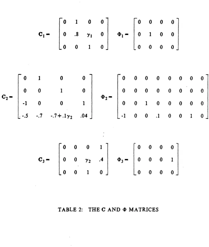
In this section we consider the problem of choosing parity functions and parity

coefficients for a 4-dimensional system operating at a set-point with two actuators and

three sensors. The system matrices are shown in Table 1. Except for two elements in

the A matrix all parameters are known exactly. These two elements are assumed to

be independent parameters denoted by Yl and y2.

Suppose we want to design a voting system for detecting a sensor failure. Three

candidate parity structures are

72( k- 2 )_]

[y2(k- 1) ly, (k-2) Y3(k- 1)

p,(k) =

a,

y2(k) p2(k) x2 [y (k -)l' p- 3() - 3(k)

;yl (k- l)

a2

|y

₁

(k-)

ay

l)

where the ai's are row vectors (of parity coefficients) of appropriate dimensions. The

corresponding 4) and C matrices are shown in Table 2. Note that each C and 4)

matrix depends linearly on either Yl or

Y2

and that the rows of C

2

are not linearly

dependent for any value of

Y2.

The parity structures under consideration do not

contain any actuator terms due to the fact that clB, c

2

B, c

2

AB, and c

3

B are all zero.

This will simplify the solution of the minimax problem without severely restricting the

discussion. Assuming a single sensor may fail, only p

3

plus pl or P2 need to be used

for residual generation (because both P

1

and

P2

include sensors I and 2). Therefore,

in addition to the coefficient design problem, we have to rank the two parity structures

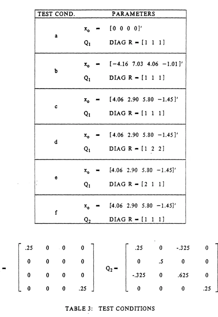
The minimax design problem has been solved for a set of six test conditions

consisting of different set-points and different plant and sensor noise intensities.

These test conditions are described in Table 3. (The two set-points are obtained by

applying ul-1 or u

2

-10 to the nominal system model.)

The nominal state

covariances Zl and 1

2

due to the two different plant noise intensities Ql and Q

2

are

listed in Table 4. Due to the simple dependence of the parity functions on the y's an

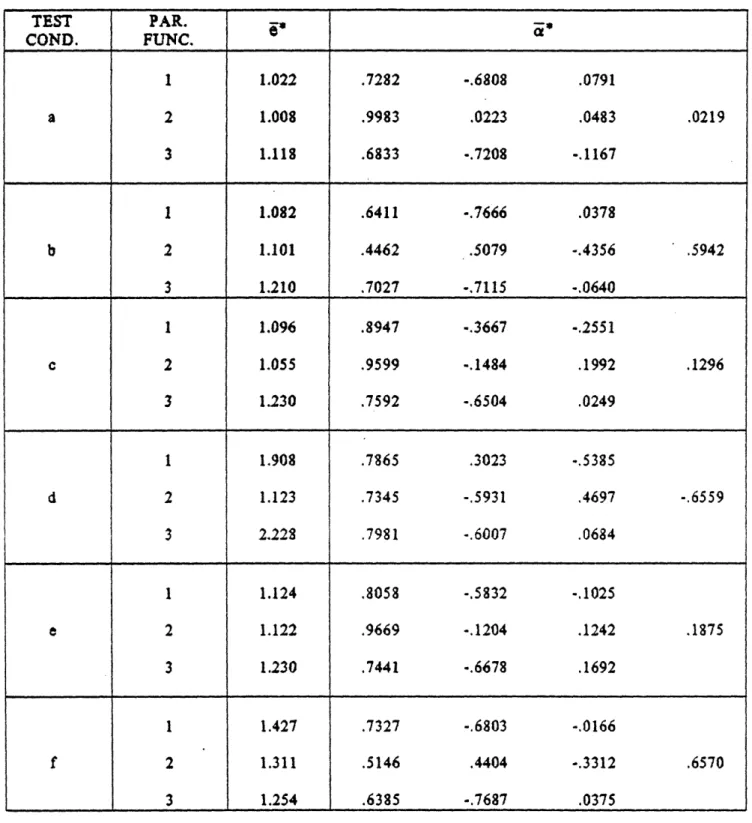
efficient solution procedure is possible [16]. The resulting parity coefficients and the

corresponding (normalized) parity errors are summarized in Table 5.

It is evident that the parity coefficients in this example are strongly dependent on

the test condition (i.e. the values of x

O

, Q, and R). Although this dependence is very

complex, some insights may be obtained from the numerical results. Consider, for

instance, PI under conditions b and c. For condition b the parity function is

p1b(k) - .6411 y2(k-1) - .7666y2(k) + .0378y I(k-l)

and for condition c it is

p

1c(k) - .8947 Y2(k-1) - .3667 y2(k) - .2551 yl(k-1)

The only difference between these conditions lies in the value of x

O

. Since the first

and fourth columns of C

1

are zero, only the second and third elements of x

O

(Xo

2

and

xo3) will play a role in the coefficient optimizaton problem. The parity function P

1

can

be written in the form

P1 ' allXo2 + a12(Xo2+YlXo3) + a13 Xo3 + 4(/l,al )

where ali, i=1,2,3 denote the elements of al corresponding to y

2

(k-1), y

2

(k), and

yl(k-1), respectively;

4

denotes the remaining noise terms. It is clear that Xo

3

and

a1 2 modulates the effect of yl on Pl. Qualitatively, as Ix,31 becomes large relative to

jxo2 (with all noise covariances the same), the optimal a12 will reduce in size (relative

to all and a13) in order to keep the effect of Yl small. As lxo3

I

increases, the signal to

noise ratio of Yl (k) also increases. Therefore, we expect 1a13 to become large to take advantage of the information provided by yl(k). Under condition b, Xo2>Xo3, and

under condition c the reverse is true. An inspection of p1 under these condition as

listed above shows that this reasoning holds. Therefore, built into the minimax problem is a systematic way of handling the tradeoff between uncertainty effects due to noise and error in system parameters.

Note that both P, and P2 relate the first sensor to the second one, and P2 is a higher order parity function than Pi. Furthermore, the rows of C2 are not linearly

dependent for any value of Y2. However, the parity error associated with P2 is smaller

than that of P1 in all conditions except condition a. This shows that a higher order

parity relation (which is more likely to contain higher order effects of y) is not necessarily more vulnerable to model errors and noise. In addition, a parity function based on a C matrix with rows that are linearly dependent for all values of y does not necessarily produce a smaller parity error than a parity function that is based on a C with independent rows.

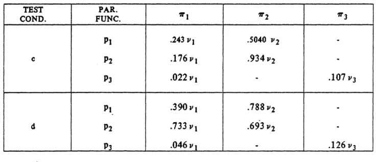
In Table. 6 we have tabulated the signature to parity error ratio associated with the three parity functions for sensor failures that are modelled by a constant bias of size vi

in the output for test conditions c and d. Here, 'ri denotes the signature to parity error ratio for a bias failure in sensor i, and it is calculated by substituting vi for yi in

determining the relative merits of pi and P2. For instance, under condition d and

assuming

vl-v2, P2 is

preferred to

pi

because it has a larger value of

irl

than

P2 while

its 1r

2

value is comparable to that of P

2

.

-VL CONCLUSIONS

In this paper we have characterized the notion of analytical redundancy in terms of a generalized parity space. We have described three methods for using parity relations to generate residuals for FDI. The problem of determining robust parity relations for residual generation using the parity function method was studied. This design task was formulated as an optimization problem, and an example was presented to illustrate the design methodology. A number of problem areas await further research. They include: a method for selecting useful parity structures for the parity coefficient problem studied in Section IV, solution procedures for the (minimax) optimization problem, and a method for determining parity relations for other methods of residual generation (i.e. the open-loop and the closed-loop methods).

REFERENCES

[1] A. S. Willsky, 'A survey of design methods for failure detection in dynamic systems," Automatica, vol 12, pp. 601-611, 1976.

[21 R. V. Beard, Failure Accomodation in Linear Systems Through Reorganization, Man Vehicle Lab., Cambridge, MA, Report MVT-71-1, M.I.T.,Feb., 1971.

[31 H. L. Jones, Failure Detection in Linear Systems, PH.D. Thesis, Dept. of Aero. and Astro., M.I.T., Cambridge, MA., Sept., 1973.

[41 A. S. Willsky and H. L. Jones, 'A generalized likelihood ratio approach to the detection and estimation of jumps in linear systems," IEEE Trans. Automatic

Control, AC-21, pp. 108-112, Feb., 1976.

[5] A. S. Willsky, E. Y. Chow, S. B. Gershwin, C. S. Greene, P. K. Houpt, and A. L. Kurkjian, "Dynamic model-based techniques for the detection of incidents on

freeways,"IEEE Trans. Automatic Control, AC-25, pp. 347-360, June, 1980.

[6] D. E. Gustafson, A. S. Willsky, and J. Y. Wang, Final Report: Cardiac Arrhythmia

Detection and Classification Through Signal Analysis, The Charles Stark Draper

Laboratory, Cambridge, MA, Report No. R-290, July, 1975.

[7] F. A. Evans and J. C. Wilcox, "Experimental strapdown redundant sensor inertial navigation system," J. of Spacecraft and Rockets, vol. 7, pp. 1070-1074, Sept., 1970.

[81 J. P. Gilmore and R. A. McKern, "A redundant strapdown inertial reference unit (SIRU)," J. of Spacecraft and Rockets, vol. 9, pp. 39-47, Jan., 1972.