Analysis, design, and prototyping of a narrowband radio for application in wireless sensor networks

Analysis, design, and prototyping of a narrowband

radio for application in wireless sensor networks

by

Fred S. Lee

Submitted to the Department of Electrical Engineering and Computer

Science

in partial fulfillment of the requirements for the degree of

Master of Engineering in Electrical Engineering

at the

MASSACHUSETTS INSTITUTE OF TECHNOLOGY

@

Massachusetts Institute

May 2002

of Technology 2002. All rights reserved.

A uthor ...

Department of Electrical Engineering and Computer Science

May 24, 2002

Certified by...

_y

Anantha P. Chandrakasan

Associate Professor

Thesis Supervisor

A ccepted by ...

...

...

Arthur C. Smith

Chairman, Department Committee on Graduate Students

MASSACHUSETTS INSTITUTE OF TECHNOLOGY

Analysis, design, and prototyping of a narrow-band radio for

application in wireless sensor networks

by

Fred S. Lee

Submitted to the Department of Electrical Engineering and Computer Science on May 24, 2002, in partial fulfillment of the

requirements for the degree of

Master of Engineering in Electrical Engineering

Abstract

In the past few years, system-level exploration of wireless data-harvesting techniques have driven circuit designers to consider power-aware radio nodes as a key component of wireless sensor networks. In this work, a discrete implementation of a narrow-band radio in the ISM band will be described. The constructed narrow-band radio achieves a bit-rate of lMbit/sec, and features a OdBm to 20dBm adjustable power amplifier. A discussion of circuits, systems, and implementation will be presented. High frequency analog design will also be discussed in detail. Finally, an analysis of the power-states and power hooks in the narrow-band radio will be explored to demonstrate a flexible, power-aware radio system design.

Thesis Supervisor: Anantha P. Chandrakasan Title: Associate Professor

Acknowledgments

I would like to thank Prof. Anantha Chandrakasan for allowing me this great

oppor-tunity to research wireless radios, build transceivers, and have a much better under-standing of RF circuits than I first did (which was close to zero knowledge) when I first joined the group. His patience, guidance, and encouragements have been inte-gral in seeing this project to the end. I am also grateful for his encouragements and guidance to me to make the paradigm shift from an undergraduate status/lifestyle of grades and classes to the graduate student mindset of research, papers, and creativity.

I would also like acknowledge the pAMPS team for their support and patience from

those many late nights of debugging, debugging, and debugging. Did I mention de-bugging? Especially Piyada Phanaphat, for her great perspective on life when things are getting down, and Nathan Ickes, for his sarcastic humor. Two great things to make late nights at lab more interesting.

Speaking of making lab a great place to be, I am thankful for the friendships of Raul Blazquez Fernandez, Ben Calhoun, Travis Simpkins, Rex Min, Alice Wang, Seongh-wan Cho, Manish Bhardwaj, Puneet Newaskar, Theodoros Konstantakopoulos, Sam Leifan, and Margaret Flagherty. They are all role models to me in many ways, pro-fessionally and personally. I am so glad that I am able to know them and that we are in the same group together.

My parents, Ken and Connie Lee, and brother, Ray Lee. Wow wow wow. Thanks for

always being there; your love and patience; and all the great food. Yum.

My apartment-mates, nori, richmoy, and j179, for being who they are, and keeping me

sane this year, with impromptu grilled-cheese sandwiches at night, late night Tekken Tag Tournament beat downs, and those times when we almost quit school and move back to Taiwan to start a band, singing Boyz II Men and Enrique Iglesias. Maybe one day... Watch for our recording.

Finally, Jesus Christ, who my life belongs to and to whom I am the father's child. These are some of my favorite scriptures.

"if we claim to be without sin, we deceive ourselves and the truth is not in us. if we confess our sins, He is faithful and just and will forgive us our sins and purify us from all unrighteousness. if we claim we have not sinned, we make him out to be a lair and his word has no place in our lives." - 1 john 1:8-10

i ain't perfect. and it's ok.

"then i saw in the right hand of him who sat on the throne a scroll with writing on both sides and sealed with seven seals. and i saw a mighty angel proclaiming in a loud voice, 'who is worthy to break the seals and open the scroll?' but no one in heaven or on earth or under the sun could open the scroll or even look inside it. i wept and

wept because no one was found who was worthy to open the scroll or look inside. then one of the elders said to me, 'do not weep! see, the Lion of the tribe

of Judah, the Root of David, has triumphed. He is able to open the scroll and its seven seals.' Then I saw a Lamb, looking as if it had been slain, standing in the center of the throne, encircled by the four living creatures and the elders... he came and took the scroll from the right hand of him who sat on the throne. and when he had taken it, the four living creatures and the 24 elders fell down before the Lamb... and they sang a new song:

'You are worthy to take the scroll and to open its seals, because you were slain, and with your blood you purchased men for God from every tribe and language and peo-ple and nation. You have made them to be a kingdom and priests to serve our God, and they will reign on the earth.'

then i looked and heard the voice of many angels, number thousands upon thou-sands, and ten thousand times ten thousand... in a loud voice they sang: 'worthy is the Lamb, who was slain, to receive power and wealth and wisdom and strength and honor and glory and praise!' then i heard every creature in heaven and on earth and under the earth and on the sea and all that is in them, singing: 'to him who sits on the throne and to the Lamb be praise and honor and glory and power, for ever and ever!' the four living creatures said, 'Amen,' and the elders fell down

and worshiped." - revelation 5

glory glory glory. and hallelujah. one day, it'll be party time. yeeeah. And now, enjoy the circuits.

Contents

1 Introduction 17

1.1 Wireless Sensor Networks . . . . 17

1.2 pAMPS Node Architecture . . . . 19

2 pAMPS Radio Power-Aware Architecture 23 2.1 W ireless Standard . . . . 23

2.2 Power-Aware Radio Transmitter Architecture . . . . 24

2.2.1 Manchester Encoding and DC Offsets . . . . 25

2.2.2 Gaussian Filter . . . . 26

2.2.3 Direct-Modulation of VCO . . . . 27

2.2.4 Power Amplifier . . . . 28

2.2.5 A ntenna . . . . 30

2.2.6 TX Power-Aware Design Summary . . . . 32

2.3 Power-Aware Radio Receiver Architecture . . . . 32

2.3.1 Low Noise Amplifier . . . . 33

2.3.2 Demodulation Architecture . . . . 36

2.3.3 RX Power-Aware Design Summary . . . . 52

2.4 Phase-Locked Loop . . . . 52

2.4.1 Power-Aware Design for PLL . . . . 60

2.5 Power States for Radio Transceiver . . . . 60

2.5.1 Control Hierarchy . . . . 60

3 Impedance Matching Circuits and Practical Implementation 3.1 Impedance Matching Circuits . . . .

3.2 Practical Impedance Matching . . . . 3.3 Transm ission Lines . . . . 3.3.1 M icrostrip Lines . . . . 3.4 Power Amplifier Impedance Matching . . . .

3.5 Low Noise Amplifier Impedance Matching . . . . 3.6 Antenna Impedance Matching . . . . 4 Other Circuits and Layout Approach

4.1 Power-Supply Decoupling . . . . 4.2 4.3 4.4 10MHz Squarewave Generator . . Oscillator Choice . . . . Layout Approach . . . . 4.4.1 Ground Plane . . . . 4.4.2 Power Plane . . . . 4.4.3 Isolation . . . . 4.4.4 Trace Sizes, Via Sizes, and

. . . . . . . . . . . . . . . . . . . . . . . . Substrate Selection

5 Experiments on Range and Power of Radio Board 5.1 Bit-Error Rate and Range Tests . . . .

5.2 Power Analysis on one Node to Node Link Using pAMPS Radio . . .

A Homodyne and Heterodyne Receivers:Tradoffs and Advantages B Matlab Files for Impedance

B.1 ustrip.m . . . . B.2 Chamcalc.m . . . . B.3 Eecalc.m . . . . B.4 Eefcalc.m . . . . Matching Calculations 63 63 67 67 71 74 76 76 77 77 78 79 79 79 80 81 82 83 6 Conclusions . . . . 83 84 89 91 97 98 99 99 100

B.5 Fcutcalc.m . . . . 100 B.6 Kcalc.m . . . .. . . . 101 B.7 Leffcalc.m . . . .. . . . 102 B.8 Lgcalc.m . . . . 102 B.9 Losscalc.m . . . . 103 B.10 Skincalc.m . . . . 104 B.11 Veldelcalc.m . . . . 105 B.12 W ecalc.m . . . . 105 B.13 Zccalc.m . . . . 106 B.14 im pedance.m . . . . 106 B. 15 quickrun. m . . . . 108 B.16 m icrostep.m . . . . 108 B.17 ustep.m . . . . 108

List of Figures

1-1 Wireless sensor network [1] . . . . 18

1-2 Node architecture . . . . 20

1-3 N ode stack . . . . 21

1-4 Top and bottom of radio board . . . . 21

2-1 Transmitter architecture . . . . 24

2-2 Circuit to remove DC offset inherent in single-supply design. . . . . . 25

2-3 3rd-order Gaussian low-pass filter . . . . 27

2-4 Power control pins for power amplifier . . . . 28

2-5 Power amplifier power consumption vs. output power . . . . 29

2-6 Antenna . ... .. .. . .. .. ... . . . .. . . . .. 30

2-7 Horizontally-aligned dipole antenna: elevation plane . . . . 31

2-8 Vertically-aligned dipole antenna: elevation plane . . . . 31

2-9 Receiver Architecture . . . . 32

2-10 Schematic for the LNA . . . . 33

2-11 SNR vs. BER plot for binary shift-keying in multiple diversity L [21] 35 2-12 Heterodyne receiver architecture with high IF frequency choice (top) and low IF frequency choice (bottom) . . . . 37

2-13 Freq vs. magnitude rejection plot [22] . . . . 38

2-14 Typical SAW filter implementation [24] . . . . 39

2-15 Discrim inator circuit . . . . 40

2-16 Bode plot of equation 2.4 . . . . 41

2-18 Key signals in tx-rx wireless link . . . . 43

2-19 Varactor diode characteristics [25] . . . . 44

2-20 LM6152 Frequency response [26] . . . . 46

2-21 Plot of AC voltage applied to varactor (C2) and AC voltage produced at discriminator output (CI) . . . . 48

2-22 Plot of AC voltage applied to varactor (C3), AC voltage produced at discriminator output (C2), and VDC (Cl) . . . . . . . . . 48

2-23 Plot of transient step response from varactor (C2) to discriminator output (C l) . . . . 49

2-24 Plot of varactor input (C2) to discriminator output (CI) . . . . 50

2-25 Root-Locus and Bode plots of feedback system . . . . 51

2-26 Frequency synthesizer circuitry . . . . 53

2-27 PLL block diagram . . . . 54

2-28 Open loop response to PLL given different charge pump gains . . . . 57

2-29 Transient responses of VCO control voltage for given charge pump gains 59 2-30 Ideal power consumption in each node state . . . . 61

3-1 Two common types of impedance matching circuits [10] . . . . 63

3-2 Types of circles in ZY Smith Chart . . . . 65

3-3 Transm ission line . . . . 68

3-4 Loaded transmission line . . . . 69

3-5 M icrostrip line example . . . . 72

3-6 M itered corner . . . . 73

3-7 Matching network for LMX2242 power amplifier . . . . 75

3-8 Matching network for Gigaant antenna . . . . 76

4-1 Power supply filters on PCB . . . . 77

4-2 Squarewave generator from sinusoid input . . . . 78

5-1 Bit Error rate test results . . . . 84

A-1 DC offset illustration

[91

. . . . A-2 Even order distortion illustration

[91

. . . . A-3 Image frequency in a heterodyne reciever architecture

A-4 IF frequency: high IF (top) and low IF(bottom) [9] .

C-1 C-2 C-3 C-4 C-5 C-6 C-7

Schematic of analog circuits for the radio board Schematic of digital circuits for the radio board PCB layout of top metal . . . .

PCB layout of gnd plane (negative mask) . . . .

PCB layout of intermediate metal layer . . . . . PCB layout of power plane (negative mask) . . PCB layout of bottom metal . . . . C-8 PCB layout of all metal layers

. . . . 116 . . . . 117 . . . . 118 . . . . 119 . . . . 120 . . . . 121 . . . . 122 123 [9] 92 93 94 95

List of Tables

5.1 Values used for variables in equation 5.1 . . . . 85

C.1 Bill of Materials for IC's . . . . 112

C.2 Bill of Materials for Inductors . . . . 113

C.3 Bill of Materials for Capacitors . . . . 114

Chapter 1

Introduction

1.1

Wireless Sensor Networks

In the recent past, wireless sensor networks have been inspired by the onset of tran-sistor miniaturization and single-chip mixed-signal integrated circuits. Public and private sectors such as the military have gained interest in the research of wireless sensor networks for the purposes of battlefield monitoring, biological/chemical de-tection, and/or reconnaissance [1]. The MIT micro-Adaptive Multi-domain Power aware Sensors (pAMPS) group was formed to research the design and prototyping of a wireless network, and to develop energy-aware techniques for such systems. The

pAMPS team is composed of people with expertise in RF, digital, software, signal

processing, and information theory.

A microsensor network is made up of many identical wireless nodes. These nodes

are scattered in an environment to be monitored with high node densities for fault tolerance, and system robustness. The network is set up in such a way that the radius of communication of each node at least intersects with one other node. Usually, these nodes are immobile and homogenous. Each node contains a processor, radio transceiver, link manager interface, sensors, and power supply. The processor is responsible for the "intelligence" of each node, and will contain the algorithms and

MAC software designed to control the entire network, allowing the network to operate

and is required to only transmit/receive short distances, due to the energy-efficient advantages of multi-hop routing in wireless networks. Multi-hop access transfers data from one node to another, until the data eventually arrives at the base-station. The base-station has the advantage of being attached to an infinite power supply. This infinite power supply allows the burden of high energy processing to be done at the base-station. Because the batteries of each node are not replaceable once they are deployed, battery regeneration techniques as well as initial battery energy densities are of great importance. Among the many types of sensors that can be placed on each node are acoustic, image, or seismic sensors [2].

B

Figure 1-1: Wireless sensor network [1]

Figure 1-1 is an example of a wireless sensor network. Each open circle in the figure represents a dead node (due to exhausting its power supply or other faults),

and each gray circle represents a node that is functional. The solid line represents the direction of travel for the source the network is tracking. The dotted lines rep-resent the direction of data hopping; the base-station, marked with B, is where the data hopping lines terminate. The concentric circles represent the sensor range. As the source moves within the network, the network dynamically reconfigures itself to

continue tracking motion, seismic changes, and/or acoustic changes. The dotted lines represent the multiple paths that the data traverses towards the basestation, so that power is conserved across the network

[11.

Figure 1-1 shows how multi-hop and multi-path techniques can be used to maxi-mize the lifetime of a network. Since the energy it takes to transmit a certain distance

r goes as r', where n is anywhere from two to four depending on the environment, multi-hop data transmission allows for lower overall network power consumption if the efficiencies for power amplifiers are high, and energy-startup costs for each node is minimal. From observing the complexity of multi-hopping networks as compared to direct transmssion, it is apparent that the lifetime of a network is less dependent on the power usage of a single node, but much more dependent on the uniform power usage of all the nodes. The more uniformly a network consumes power, the longer the lifetime of the network [1]. Furthermore, the figure shows fault tolerance, which is somewhat similar to the independence of a network's lifetime from the lifetime of a single node. Since there are many paths that data can travel to and from the base-station, there are few "critical paths" where if a node dies, then many other nodes can no longer communicate with the base-station. In effect, the more interconnected the nodes are, the more fault-tolerant the network is. More information on network lifetime can be found in

[1].

1.2

pAMPS Node Architecture

Figure 1-2 is a block diagram of the node's architecture. In actual implementation, the hardware for the nodes are divided up as such: the processor board contains the

DC/DC converter and processor; the sensor board contains the battery and sensors;

and the radio board contains the radio transceiver, PA, LNA, antenna, and Link Manager Interface (LMI). The radio transceiver board is the focus of this work. The key difference of this radio from others is the addition of power-aware circuits, in

addition to the traditional RF circuitry. This allows for minimal power consumption from an intelligent management of energy. The specifications for the uAMPS node

Battery & Radio 0- PA

DC/DC Conv Transciever NA Data

-- --- --- To/From

Other

Nodes

StrongARM Link Manager

Processor Interface

Sensors 90

Figure 1-2: Node architecture

are as follows:

" (55mm)2 board space for each stack " low power operation, with power hooks

" ability to accommodate spatial density of 10nodes/m2

" tx/rx distances from 10m to 100m

The power hooks are power controls for the radio states, output power levels, and different states including idle and off. In a combined effort of numerous graduate students [3] [4], the node is implemented in the MTL laboratories, meeting the above specifications, as pAMPS node 1. A picture of the actual implementation is in figure

1-3.

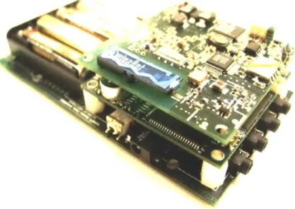
The focus of this thesis is the design of a power aware narrow-band transceiver. Figure 1-4 is the radio board that was constructed.

4

Figure 1-3: Node stack

Figure 1-4: Top and bottom of radio board

Chapter 2

ptAMPS Radio Power-Aware

Architecture

This chapter outlines the system-level considerations for the narrow-band radio that is implemented in the pAMPS node. Different from most radio transceivers, this radio has high compartamentalization and many power-aware hooks to turn on and off different sections and states of the radio, to allow for power-aware operation. The radio core is National Semiconductor's LMX3162 radio transceiver chip. Many blocks are a hybrid of on-chip (LMX3162) and off-chip discrete components. This chapter serves to outline the basics of the wireless standard, radio architecture, and power control hooks.

2.1

Wireless Standard

As with most commercial transceivers, this radio is built in the Instrumentation, Scientific, and Medical (ISM) band. First of all, there are no restrictions on who may operate in this band. Secondly, the ISM band is in the 2.4GHz to 2.48GHz range,and requires power emissions below 20dBm. This limitation in power output does not affect the specifications for wireless sensor nodes, because wireless sensor nodes do not need to transmit very far distances. It is possible to calculate the necessary receiver sensitivity from the power limit in order to transmit the maximum

desired distance of 100m between two nodes. The minimum sensitivity of a wireless

receiver in this network can be calculated using the Friis Transmission Equation

[51:

P, A 2

= GotGo, (2.1)

P 4TrR

In equation 2.1, Pr represents the power received at the receiver (also the receiver sensitivity, if expressed in dBm), Pt is power transmitted at the transmitter, A is wavelength of the RF signal, and R is the distance between the transmitter and receiver. Finally, Got and Go, are the gains of the transmit and receive antennas. It is important to keep in mind that this equation does not take into account possible impedance mismatches from the PA/LNA to the antenna. If the antennas are assumed to be isotropic, then Got and Go, are equal to 1. Using the equation and setting the frequency to 2.45GHz, a receiver sensitivity of -60.225dBm is required to receive the 20dBm signal at 100m from the transmitter. For the uAMPS radio, a Bluetooth-compatible transceiver chip from National Semiconductor was chosen to serve as the core of the radio transceiver [6]. The architecture of this chip, the LMX3162, and surrounding circuitry to construct a radio, will be discussed. next section.

2.2

Power-Aware Radio Transmitter Architecture

TX

datafrom

Link

Manager

R

PLL

X 2

Mtwork

P

Ntwork

Interfaice

(Xilinx)

Ref Clocki

Figure 2-1 is a block diagram of the uAMPS radio architecture. Starting from the

TX Data in figure 2-1, the signal path for transmission can be traced.

2.2.1

Manchester Encoding and DC Offsets

The binary data is fed through the 3rd.order Gaussian filter, from the Xilinx FPGA. It is important that the average DC voltage of the this data is immobile, with respect to time. If the data is encoded using Manchester encoding, then the data is guaranteed to have approximately equal numbers of upwards edges and downwards edges, at any given time. The importance of the DC voltage being immobile, lies in the fact that when the system is used in direct modulation, it is desired that only high frequency (the encoded data) be translated to the PLL. If DC components or low frequency components are also sent to the PLL, then the response of the loop to correct for this

DC offset results in longer settling time. All of these add to reduce the probability

of data recovery. So, this is why Manchester encoding is important. However, this does not solve the entire problem; because the data coming out of the radio is from a single-supply design, the OV to 3V transitions hold a DC offset of 1.5V in steady state. To remove this DC offset, a simple circuit shown in figure 2-2 is used to remove this DC offset inherent in the single-supply design side-issue, before the Manchester encoded data is sent into the Gaussian filter. The way this circuit works, is that

Fthom DC

L

4CO input

Fom C impedanice

ofA el correction

Circuit _{C, C}

k

Figure 2-2: Circuit to remove DC offset inherent in single-supply design.

when there is no data being transmitted, the voltage level of TXDA TA HIGH is set to be 3V, and the voltage of TXDATALOW is set to be OV. Through the 500Q resistors, the impedance looking to the right of the voltage divider at DC is 6.2kQ,

since the input impedance of the VCO input is 4kQ. Since the impedance looking to the right of the voltage divider is more than a decade above the resistor divider leg that it is in parallel with, the DC voltage that can be approximated at the divider is 1.5V. At the input of the VCO, the voltage is attenuated by 2.k 4kr, giving a voltage

around 0.9V. When it is desired to transmit data, the voltages of TXDA TA HIGH and

TXDATALOW are tied together in the Xilinx, thus further reducing the impedance

between the left of the 2.2kQ resistor to the input from the Xilinx. This impedance difference allows for a rough estimate that voltage drop across the 500Q resistors in parallel is zero. When 3V and OV is applied to both of the Xilinx outputs, the voltage that appears at the VCO is +/-0.9V. Hence, the DC offset problem has been resolved. The 2.2kQ resistor also acts as a gain control resistor; if the bandwidth of transmission needs to be increased, all that needs to be done is to change the value of the resistor. The only caveat is that the smallest value for this resistor needs to be no less than lkQ for the above approximations to hold true. But the good news is that since the frequency/voltage constant of the second VCO input is relatively high, to have a maximum

+/-0.2V

voltage swing at the VCO input will force an increase in this resistor size. in addtion, the 2.2kQ resistor sets one of the three poles that are associated with the 3rd-order Gaussian low-pass filter. Thus, at high frequencies, there could be some low frequency filtering/amplitude degradation due to a pole entering into the picture earlier than expected. Even though this may seem like a negative effect (our Gaussian filter is no longer a true Gaussian filter because one of the poles appear in a different place), this actually helps to solve inter-symbol interference problems. By experimentation (a potentiometer), the optimal value for this resistor was found to be 2.2kM, as stated in this explanation.

2.2.2

Gaussian Filter

2-3 is the schematic for the Gaussian filter. The Gaussian filter is required for

Gaus-sian frequency-shift keying (GFSK) data transmission to create GausGaus-sian pulses. As shown in figure 2-3, the input impedance of the second control pin of the VCO to allow for a direct-modulation transmitter architecture has a resistance of 4kQ. This

Fromi DC LVCO input romDC Linpedance

offtel correction

circuit C1 C, 4kQ

Figure 2-3: 3rd-order Gaussian low-pass filter

resistor, along with C1 (which is valued at 50.6pF), sets one of the three low

fre-quency roll-off poles. The other two poles to cause severe 3rd-order low-pass filtering are caused by L and C2. The voltage divider of 4kR sets the DC attenuation of

the data from the input to output of the filter. The values L and C2 are lmH and

390pF, respectively.

2.2.3

Direct-Modulation of VCO

After the Gaussian pulses are generated, These pulses of data are fed directly into the second modulation pin of the VCO, which is already serving as the VCO for a

1.2GHz phase-locked loop (PLL). This second input pin through the external VCO

that directly modulates the output frequency in an additive manner to the main

VCO output that is embedded in the PLL has a much lower frequency/volts

con-stant than the portion of the VCO that serves the PLL. The second input pin has a frequency/volts constant of 1.25MHz/V, while the portion of the VCO involved in the PLL has a frequency/volts constant of 60MHz/V. This makes sense, be-cause the VCO needs to span over 100MHz in frequency band, centered at 1.225GHz which the 60MHz/V constant allows. On the other hand, for a direct-modulation scheme, the frequency/voltage constant needs to be small, to allow narrowband direct-modulation. The actual PLL and mechanics of direct-modulation will be de-scribed in detail in a later section of this chapter. By providing a Gaussian pulse that has an amplitude of 0.2V, to the second input pin, The data is frequency shifted

radio chip shifts these frequencies up to

+/-500kHz,

centered about 2.45GHz.

2.2.4

Power Amplifier

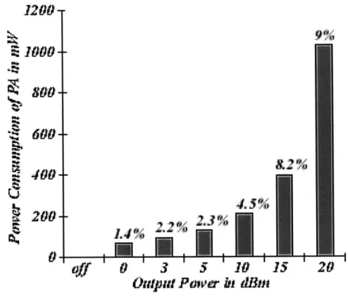
After a set of matching networks (detailed description in Chapter 3) external to the LMX3162 chip, the 2.45GHz signal is sent to the external power amplifier. This external PA has a coarse power control embedded in its on-off switch. In the off-state, the PA draws only 0.5jpA, or 1.7puW on a 3.3V power supply. When the PA is on, it is adjustable between six output levels: OdBm, 3dBm, 5dBm, 10dBm, 15dBm, and

20dBm. These power control levels are easily interfaced to the Xilinx board; figure

2-4 shows how this is done with the Xilinx in an open-drain output configuration. In figure 2-4, the voltage Vaobas is set internally by the MAX2242 power amplifier.

Figure 2-4: Power control pins for power amplifier

Thus, when the control voltages for any of the transistors on the Xilinx FPGA are pulled high, the MOSFET becomes a short, and bias current is forced down the resistor. since Vpabias is fixed, the bias current is sensed by the PA, and multiplied

by a constant, accordingly. Due to non-zero source impedances of voltage sources,

this bias current-to-output power relation is linear for only a small range. In the opposite case, when the voltages at the transistor gates are high, the MOSFETs are open-circuited, thereby disallowing any bias current to be drawn out of Vpabias. In

this manner, shorting only one transistor at a time, it is possible to set six output power levels for the power amplifier. The values for the resistors that were obtained

R2 = 165KQ for OdBm output power

R3 = 140KQ for 5dBm output power

R4 = 100KQ for 10dBm output power

R5 = 40KQ for 15dBm output power

R = 8KQ for 20dBm output power.

The power consumed by the power amplifier alone in each of these states is shown in figure 2-5. The percentages above the bars represent power amplifier efficiency'.

1200--E 1000 .4

200--

₂

_2.3

60-off

0

3

5

10

15

20

OIpII

Powe

i dhim

Figure 2-5: Power amplifier power consumption vs. output power

Finally, after another matching network for the antenna, the signal radiates into the air according to the characteristics of the antenna. A 3-d plot of the radiation pattern of the antenna is shown in figure 2-6(a). The impedance matching circuit for

(a) Antenna 3-d radiation pattern (b) Antenna shape [16] [16]

Figure 2-6: Antenna

2.2.5

Antenna

The antenna that is used is a a !-wave, horizontally-aligned antenna designed by

GigaAnt [17]. The radiation pattern is theoretically omnidirectional, has a gain of 4dBi (betraying a hint of signal directivity despite omnidirectional claims), and has

an efficiency of 62% [16]. As can be seen in figure 2-6(a), the antenna actually has high directivity in the Z direction, which is unwanted if a high lateral transmission radius is desired. The elevation radiation pattern for a traditional antenna dipole that is horizontally-aligned is in figure 2-7. It is apparent that the gain at 90' is already very small, compared to the gain at 00. The solid line represents the radiation pattern due to a solid ground plane, and the dotted line represents the radiation pattern due to an earth ground [5].

A good candidate for a replacement antenna would be a normal !-wave

vertically-aligned hertzian dipole antenna on a ground plane. The radiation pattern of such an antenna shown accordingly in figure 2-8. The solid line represents the radiation pattern due to a solid ground plane, and the dotted line represents the radiation pattern due to an earth ground. The drawback to a vertically-aligned antenna is that the radio board profile is no longer low-profile. Loop antennas (square or circular) are

'PA efficiency is radiatedpower/powerconsumed

... .

90 90

Figure 2-7: Horizontally-aligned dipole antenna: elevation plane

good candidates for horizontally-aligned antennas that have good lateral radiation. The downside is that the output coupling of the antenna to the circuit needs to be fully-differential. However, by using a balun, the single-ended signal would be able to couple with fully-differental circuits [5].

In real life tests, it is found that for a -wave antenna, the radiation pattern has great dependency on ground plane location. It is found that it is necessary for the node to be a foot or more above the ground plane for proper radiation; otherwise, at 3dBm of output power, the receiver is unable to receive when the nodes are more than a few feet apart, flush against the ground. It is difficult to measure and model such radiation patterns and strengths, so it is by trial and error, experience, and time that antennas are properly designed.

0

30 Ulfin ,

90 90

2.2.6

TX Power-Aware Design Summary

The LMX3162 also has a TX_PD switch that switches on and off the internal cir-cuitry needed for the TX path. This power hook, in addition to the ones previously mentioned on the power amplifier, constitute the power management control pins for the transmitter, and allow the transmitter to be offered as a black-box with these simple control lines so that the system and network designer may have easy access to these power-aware features.

2.3

Power-Aware Radio Receiver Architecture

RX data to

L ink Manager

Interface

(Xilinx)

Matching LN A Matching Network IN NetworkI BPF

X SAW f _{X SAWfiltr} ~IFr _Am Auto-Calib,.. f,

Discriminator

PLL

10MHz Rcf Clock

Figure 2-9: Receiver Architecture

Figure 2-9 is a block diagram of the uAMPS radio receiver architecture. After elec-tromagnetic waves are received onto the antenna, the antenna feeds to the matching network of the low noise amplifier (LNA).

2.3.1

Low Noise Amplifier

The key characteristics of the LNA are low noise and high linearity. For discrete LNA design, much like the PA design, care has to be taken for power supply filtering and ground layout. The matching networks will be described in Chapter 3. The circuit for the LNA is shown in figure 2-10. The LNA is implemented using Siemen's BFP420

Rb

Cp,

-Rbias L

Matching Network

Network

Figure 2-10: Schematic for the LNA

RF silicon transistor. This transistor runs off of a regulated supply coming from the LMX3162. This regulated supply was designed to be used by an external LNA. In addition to being off-chip, the advantage of having the LNA power supply controlled

by the LMX3162, is that a free power hook is available for use. mirroring the TXPD

pin, There is a pin on the LMX3162 called RX_PD that turns on and off the internal circuitry related to receiver circuits, as well.

Looking at the schematic in figure 2-10, a walk-through of how this circuit works is as follows. Rb is chosen to provide proper collector-emitter biasing at 2V from a 3V power supply. The base current is set by Rbias to be Ic/beta, where I, is desired to be 20mA and beta of the transistor is typically 80. The matching network to the left of the circuit contains a AC coupling capacitor to prevent bias current flowing into the antenna. The resistor Rb can be tweaked, depending on the actual Vc, value, to obtain correct current values. The power supply for the LNA comes

from an internal regulator inside the LMX3162; this regulator provides 2.7V. By reducing Rb, better performance for the LNA is obtained. A measured gain of

10-12dB can be obtained in this fashion. With more complicated test equipment and

setup, the actual S-parameters could be measured, and exact optimization of the LNA could be obtained; however, since this particular component has reliable specification sheet data and pre-measured data, it is possible to rely on this pre-measured data to optimize the circuit to a desirable quality. Another advantage of reducing Rb, is that it minimizes the negative feedback effects that the output incurs at the input. When large currents are drawn in the transistor, the transient response of Ic becomes large in magnitude. This causes a larger voltage drop across Rb, thereby reducing the voltage across Rbias. With the reduction in voltage drop, I, is reduced through the reduction if b. Effectively, reducing Rb reduces the gain of this unwanted minor loop

feedback effect [7] [20].

The noise factor of the amplifier is at a minimal 1.5dB. The receiver sensitivity can be calculated using equation 2.2 [20].

Pin,min = -174dBm/Hz + NF + 10 log B + SNRin (2.2)

-174dBm/Hz is the amount of noise power per unit bandwidth that the source

resistor delivers to the input. SNRmin is related to a desired specification for bit-error rate. This correlation is shown in figure 2-11. The bandwidth B is expressed in

Hz, and is set from the beginning. Noise factor is the equivalent noise factor of the

entire receiver chain. The noise factor of a cascade system is generally most highly impacted by the first circuit block [9]. Thus, for a given desired BER, a SNR can be determined. Noise figure is constrained by and a sensitivity can be calculated from equation 2.2. Using the path fading equation (eq. 2.1), it is possible to obtain the approximate distances the wireless link can transmit.

Linearity is determined by input matching over a frequency range, and minimal phase changes in the frequency on interest. Linearity is also affected by the non-linear

\

\

tb-cl

I I I I 0 5 10 15 20 25 30 35 40 SNR (decibels)

Figure 2-11: SNR vs. BER plot for binary shift-keying in multiple diversity L [21]

10 10 10 in10 10 10 10 i I i I I i \

that increases linearity of the amplifier over a larger signal swing. Large signal swings also change the values of junction and diffusion capacitances of the transistor. IIP3 is a good method that benchmarks the linearity of the circuit, while also allowing different amplifiers to be normalized by their own 3rd-order intermodulation products so that their linearity performance may be compared to another amplifier. IIP3 is the

amplitude of the input when the output fundamental component intersects the ₃rd_

order intermodulation product of a two-tone input test. Usually a good approximation

for IIP3 can also be obtained if the 1dB compression point is known. Equation 2.3

shows this relation [9].

AI = A1dB - 10dB (2.3)

The 1dB compression point is the input at which the output gain drops 1dB below

the ideal gain across all amplitudes of input. For this LNA, the 1dB compression

point occurs at 12dB and IIP3 at -8dB [20]. It is interesting to note in passing that this LNA can also be used as a power amplifier, with maximum output gain of 12dB. Following that analysis, a more practical use would be to use it as a pre-amplifier for

the MAX2242 power amplifier.

2.3.2

Demodulation Architecture

The LMX3162 is built to support heterodyne demodulation, with IF frequency se-lected at 110.6MHz. Heterodyne systems are much easier to implement than homo-dyne (or direct-conversion) systems, because homohomo-dyne receivers have the following three problems, which by adopting a heterdyne architecture, can be avoided: [9]:

" DC offsets in analog demodulated signal

* Even-order distortion

" Flicker noise.

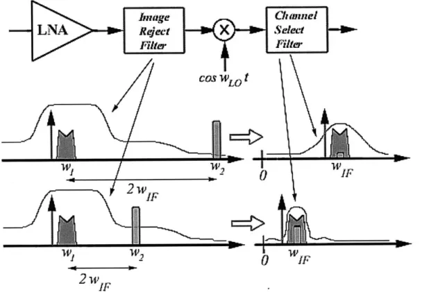
Figure 2-12 shows the heterodyne receiver architecture with corresponding frequency-domain plots to show image rejection, channel selection, and interferer rejection abil-ities of the receiver depending on the choice of a low or high IF frequency. For further

information on the tradeoffs and benefits of a heterodyne architecture, see Appendix A for a systems-level explanation of the IF frequency, associated filters and circuits, and a comparison to direct modulation architectures.

1umage Charmnel

LNA

Jkeet

,

X

select

Niter Filiff COS I LO t W 2

0

IFIF 2

_w2r

Figure 2-12: Heterodyne receiver architecture with high IF frequency choice (top) and low IF frequency choice (bottom)

Image-Reject Filter

The image reject filter is built by Murata, using high dielectric constant ceramics to provide ultra-high

Q.

The input and output impedances of this circuit are already matched to 50Q, so there is only the need for coupling capacitors and matched trans-mission lines. The bandwidth of this circuit is 84MHz centered at 2.442GHz, giving a

Q

of 29. The bandwidth of the image-reject filter also helps determine the IF fre-quency that should be chosen. Since the IF frefre-quency that is chosen is 110.6MHz, it is easy to tell from figure 2-13 that the largest possible image magnitude that will be folded back onto the wanted signal by the mixer is more than 20dB below the

0: 20-*40 C a) 60 0 T 10 20 30 0 80 1 40 2000.0 2500.0 3000.0 Frequency (MHz)

Figure 2-13: Freq vs. magnitude rejection plot [22]

magnitude of interest.

Mixer, PLL, SAW filter, and IF Amplifier

Since most of these components are on chip, their discussion will be brief. The mixer has two inputs, one of which takes as input from the received signal, and the second input takes the generated frequency from the PLL as input. The PLL frequency does the channel selection; basically, it generates a frequency that is 110.6MHz less than the desired band to receive and demodulate. The output of this mixer will have sum and difference frequencies; the sum would send the amplitude peak in the frequency domain to 5GHz, which will probably be attenuated anyway, since the world is low-pass in nature. The difference will be at the IF frequency: 110.6MHz. After this IF frequency is generated, it is desirable to put the signal through a very high-Q filter. High-Q filters can easily be generated by Surface Acoustic Wave (SAW) filters.

This type of filter converts electromagnetic waves into acoustic waves by activating a piezo-electric structure. In figure 2-14, the grill-like objects are called inter-digital transducers (IDT) that are on a piezo-electric substrate, which transforms electro-magnetic waves into acoustic waves, and vice-versa. The geometries are of key

im-Ods -6 dU

Acoustic Absorker Acoustic Absoder

Figure 2-14: Typical SAW filter implementation [24]

portance to determine frequency selectivity, delay, and fundamental frequency. The

key advantage of SAW filters is their ability to produce an ultra-high

Q

and frequency selectivity. However, losses are usually associated with saw filters, due to the lack of directivity for acoustic waves exiting the IDTs. SAW filters also exhibit linear phase modeled as a pure delay. Sometimes SAW filters are also used to create delays. Because of this delay feature, the impedances of SAW filters cannot be measured by a traditional ohmmeter. However, since S-parameter analyses are based upon ratios of voltages, it is possible to measure S11 and S22 of a SAW filter and back-calculate the input and output impedances, respectively [24].

The SAW filter that is used for the IF frequency is centered at 110.6MHz, and has a

3dB bandwidth of 1MHz. At +/-1.150MHz of the center frequency, the attenuation

is already 10dB. At +/-3.456MHz of the center frequency, an attenuation of 40dB is

achieved. The

Q

of this device is above 100. After the channel select filter processes

the signal, it is sent to an on-chip IF amplifier that gives 70dB of gain, and then fed into the discriminator circuit [23].

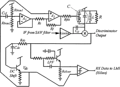
Discriminator and Demodulation Circuitry

The discriminator circuit works as follows. From the IF amp, the signal is sent into

the multiplier shown in figure 2-15. At one input to the multiplier is the original signal. The second input passes through a filter, which has the following transfer

Ce _"

cc]c biX/l/nx)J

-) + 2 fll)L *R

Rbie,2 RiA

Fiur 21:Drimnao ccu i ciiao

~ Nfrom SA Wfifter Ct X otpuiito

Rdc C 2 LC s2RL(C + Ns R(24 LPF 0 dc RX D a ta to Lai DCRsce Shift

Figure 2-15: Discriminator circuit

function:

2 8 2RL~c(2.4)

s2RL(Cc + C)sL + R

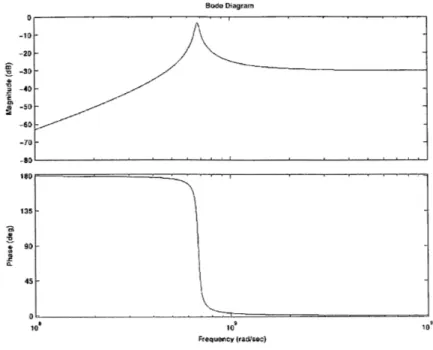
Figure 2-16 is the plot of the transfer function of equation 2.4. A description of the circuit follows.

Cc is internal to the LMX3162, and is set to be 1pF. The other passive

com-ponents are all external. The capacitor that is above the varactor in figure 2-15 is set to be in the nF range, so that the effective impedance of that series capacitor connection is dominated by the varactor. The varactor is used to fine tune the reso-nant peak that the larger capacitor to the right of the series capacitor network and inductor form. The resonant peak is desired to be at 110.6MHz so that the phases at 110.6MHz-/+500kHz are at 180 and 00 respectively. This phase difference can be seen on figure 2-16. The resistor R is not explicitly placed in the circuit, but

comes from the

Q

of the inductor (i.e. - series resistance). Typically, an inductor

has an associated series resistance. For narrowband analysis, the series R-L network can be broken into a parallel R-L network. The associated equations to do such a

Bodo Diagram 0 --20 --30 S-40 1 50 -60 -70 -00 135 45 -0* 100 10 1010 Frequency (raM/sec)

Figure 2-16: Bode plot of equation 2.4

transformation are described below

[10].

WLseries

Q series -Rseries (2.5)

Rparaiei = Rseries(1 + Qsiries) (2.6)

1

Lparaiie= Lseries(1 + 2 ) (2.7)

Qseries

Thus, R is the same as the Rparaiiei calculated in equation 2.6. The tradeoff is

as follows. The higher the

Q

(smaller the series resistance), the more "peaky" figure

2-16 becomes. This peakiness translates to greater SNR, but also creates harmonic

distortion, due to the 40dB/decade rollup and peaking of the circuit. Lower Q's decrease the SNR, but create less harmonic distortion, since the magnitudes at

+/-500kHz of the center frequency are likely to be more matched.

The way the discriminator circuit works to recover the baseband signal is as

fol-lows. When the discriminator is tuned at 110.6MHz, the phase sits at 900 at that

frequency. The mixer takes two inputs. If the frequency that is generated from the

means that the mixer inputs are directly opposite of each other in sign. When op-posite sinusoids are mixed together, the result is a lower DC-average value at the output. If the frequency that is generated from the IF amplifier is at 111.1MHz, the discriminator essentially does nothing dramatic to the phase and frequency of the signal, so the two inputs to the mixer are the same. When two sinusoids of same sign are multiplied, then the average DC value of the output is high. Thus, by filtering out the "carrier frequency" between 110.1MHz and 111.1MHz, the baseband at 500kHz can be recovered, represented by the "average DC value" of the output of the mixer. Figure 2-17 shows the results of input frequencies at 110.1MHz and 111.1MHz

[7].

7

In phase signals

5--

4-

3-Out fphas Signals

0.5 1 1.5 2 2.5 3 3.5 4 4.5 5

time _{X 10}

Figure 2-17: Time domain plot of discriminator response to two frequencies

Figure 2-18 is a plot of the transmitted bits from a radio that is configured to transmit, the Gaussian-filtered Tx data, the recovered analog signal from the dis-criminator of the receiver radio board, and finally the recovered bits back into the digital domain. The digital bits are delivered to the Gaussian filter input via the Xilinx FPGA. The Gaussian filter feeds directly into the VCO, via a second control input that has a much lower frequency/voltage ratio. The Gaussian filter changes the square wave into a Gaussian symbol, which is more band-limited than the

frequen-cies produced by square waves. This reduces inter-symbol interference, and limits the bandwidth of transmission to the desired 1MHz. The demodulated signal on the third channel is read at the output of the discriminator mixer. The recovered data can be compared to the signal on channel two. Finally, the digital bits are generated from a bit slicer circuit, employing a properly damped comparator. If the duty cycle of the recovered digital data is not 50%, it is possible to change the resistor value of Rsicer in figure 2-15 such that the comparator is given correctly-balanced voltages so

that the slicer is able to recover bits correctly. The 2nd-order filter that is connected

to Rsiicer removes unwanted high frequency harmonics, so that the slicer does not

decode wrong edges. The requirement for the DC-shift of the emitter-follower on the

DC reference signal is necessary, because the demodulated data is also shifted by a Ve

drop of a transistor. The DC reference signal, as seen in figure 2-15, is generated by a low-pass filter. This low-pass filter affects the settling-time of the recovery circuitry, as it takes approximately 4T of the time constant of the low-pass filter to settle to the correct DC-average value. The other surrounding circuitry is the analog feedback loop to control the varactor and automatically tune the circuit to 110.6MHz.

Stop.,Singie Seq SOOMS/s

Figure 2-18: Key signals in tx-rx wireless link

Going back to figure 2-15, the varactor can be implemented in two ways: a physical hand-tuneable variable capacitor, or the series connection of the two capacitors with a

varactor diode. The reverse-bias voltage drop of the varactor changes the capacitance of the diode. The graph in figure 2-19 shows the typical capacitance vs. voltage characteristics of the varactor.

10.0 C 8.0 0. S4.0 2.0 ft 0 1 2 3 4 5 Varactor Voltage (V) Capacitance vs. Voltage

Figure 2-19: Varactor diode characteristics

[25]

Because the curve in figure 2-19 is not constant, and there are inconsistencies in reference oscillators, etc., it is of great advantage to remove the hand-tuning capacitor and replace it with a diode varactor embedded in a feedback loop to automatically tune the circuit.

The feedback circuit follows from figure 2-15. The values for the circuit are as

follows: Rbiasl = 5.86kQ Rbias2 = 3.47OkQ Cc =1OuF Ri =1kQ Rf = lOkQ Rf~it = OQ Cto0 fdiode = 4.7nF Cdiode = 2 - 9pF Ctank =1 8pF

L = 68nH

Rd, = 5kQ

Cdc = 2.7nF

RDCshift = lkQ

Rsuicer = lkQ

A brief intuition on how the feedback loop works is as follows. Beginning with

the discriminator output, there will be some baseband Gaussian- modulated signal centered around 500kHz. there is also a DC offset associated with this signal. The low pass filter formed by RDC and CDC is set at 11kHz (the plots that reveal this will

be described in the detailed analysis to follow). This effectively filters out the high frequency component of the discriminator output, and captures the DC offset value, but still containing low frequency (below 11kHz) noise. The interesting problem to note about this filter is that if the filter pole is set to be very low to filter out more of this unwanted noise, the transient settling time increases, since setting time is the

same as 4 1 -. If the pole of the filter is increased to decrease settling time, it

is obvious that this would allow more ripple to appear at the ideally DC voltage level. This problem will be dealt with later. Continuing down the signal path, the transistor that performs the DC shift is important, because the LPF transistor introduces a Ve

drop to the DC value of the recovered Gaussian pulses. In order for the comparator to slice the discriminator output at the midpoint, the DC offsets for Vdc and the filtered discriminator output must be the same. As said before, if the DC offsets are not exactly the same and the output of the comparator is not 50% duty-cycled for a 1-0-1-0-1-0 data transmission, then Rslicer can be changed slightly, to twiddle the bias current through the transistor so that the Ve drop will be the correct value to produce good results. The reason the resistor at the base of the DC shift transistor is not adjusted is because that transistor and those circuits are embedded in a feedback loop, which would cancel the very changes that need to be made. The opamps that are used are fromNational Semiconductor, and are their high performance JFET-input, ultra-high gain-bandwidth product LM6152 opamp

[26].

The frequency response for

the op-amp is shown in figure 2-20. If the opamp is put into unity feedback to act as 0 a' (I' a-z

Open Loop Gain/ Phase (Vs = 5V) 120 ""k" (Pha - _ _ 1M (Ph 80 60 40 20 1M (Gain 0

10k look IM loM looM

FREQUENCY (Hz)

DS01 2350-24

Figure 2-20: LM6152 Frequency response [26]

a buffer, it is easy to tell from figure 2-20 that the circuit is able to operate well up to

20MHz. Thus, it is possible to assume that the follower, or even a gain of 10 stage

that is built with this opamp, is reliable. No other dynamics need to be included from this opamp, due to its high-bandwidth response relative to the unity-gain frequency of the entire loop, which will be discussed in the detailed description [26}.

Opamp A1 is put into a unity gain configuration. The voltage that is produced

by Rbiasi and Rbias2 is the DC offset voltage that the discriminator and VDC should

be at. It is possible to use this DC voltage as a reference, instead of trying to correct the frequency error that the tank generates. The reasons to use this voltage are:

" the voltage is already here to analyze

" analyzing absolute frequency offset does no good to actual performance/ability

to demodulate the IF to baseband, because difference in oscillator frequencies may cause a shift in the IF frequency

" analyzing the DC offset is the farthest variable before entering the slicer that

we can embed into a feedback loop to gain noise immunity characteristics of feedback loops.

se)

Next, it is interesting to note that what is generated at the input into opamp A1 are

two-fold. Firstly, it is to generate and buffer a solid reference for what VDC should be. Secondly, it is to include the low frequency components of the real VDC, so that when the comparision (error generation) of VDC to this reference is made in A2, the

low frequency ripples will not cause the output of the subtractor to oscillate and/or saturate. Opamp A2 is set at a gain of 10, using resistors Rf and Ri. Finally, Rfilt

is set to be OQ. The idea of Rfgit is to allow for dominant pole compensation, if further compensation is needed. A2, as stated before, also does the subtraction/error

generation, and amplifies the signal. This subtraction is positive so that is why the positive terminal of the opamp is not to ground. The reason the subtraction must be positive, is that the sign of the gain for the diode voltage to the discriminator output is negative. When the signal is changed from the varactor voltage to the discriminator output, the feedback loop is closed, a negative sign is inserted into the loop, and there

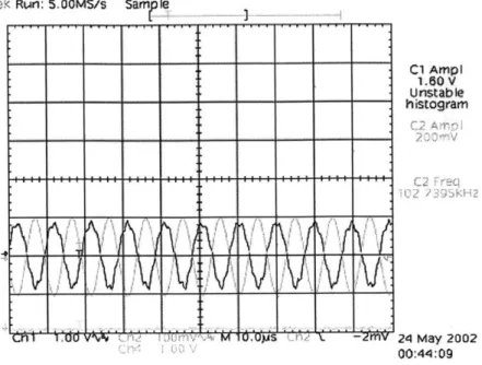
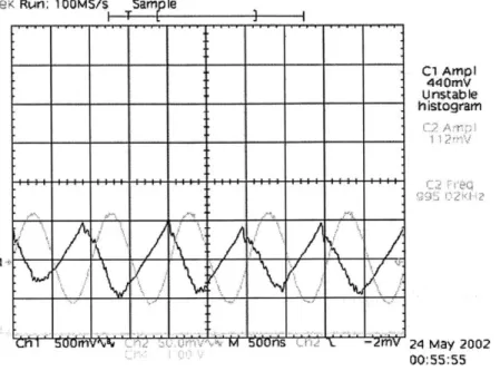
is a control circuit that exists to set the DC value of VDC, and reflected back to the discriminator output, to a useful value so that the data can be correctly sliced and regenerated into the digital domain by the comparator that feeds to the Xilinx FPGA. The most interesting part of the feedback loop is figuring out the transfer function between the discriminator output and the varactor voltage. An experiment is set up to analyze this transfer function. In this experiment, one radio node is set to con-stantly transmit at a set frequency, and the LO of the receiver is set to be 110.6MHz lower than the transmitter frequency. No data is transmitted; just the fundamental frequency. Secondly, a function generator is connected to the varactor voltage. The correct DC value is generated to the varactor so that the discriminator output sits at 1.5V, the "sweet spot" for maximum output demodulation amplitude and phase discrimination. Then, a sinusoidal signal is added onto the DC voltage of the varac-tor. At low frequencies, when analyzing the AC signal at the discriminator output compared to the AC signal at the the discriminator output, a gain of -8 is observed. Figure 2-21 shows a measurement made at low frequency. The input frequency is swept at the diode until around 700kHz, when a noticeable drop in gain begins to creep into the circuit. Figure 2-22 shows this pole location in phase and magnitude.

Te: Run: 5.OOMS/s C1 Ampi 1.50 V Unstable histogram 02 Amr"i 2 0V i

Mm

Figure 2-21: Plot of AC voltage applied to varactor (C2) and AC voltage produced at discriminator output (CI)

Te< Stop: 25.OMS/s

.1-; g L"s t F 1

it

1

;

M e it hi-I;m

/-I n% dm s 0h3 1 00 V

Figure 2-22: Plot of AC voltage applied to varactor (C3), AC voltage produced at

discriminator output (C2), and VDC (Cl)

24 May 2002 00:44:09 : 80mV :1.04JaS -20mV C1IAmpl 72mV Unstable histogram C2 C3-4C2 Oha U nstablip h stoyram 24My 2002nf 02:03:36 Sample I c m: i on