Bayesian analysis of crime rate changes in before-and-after experiments

(1)

!2yr,, '0"0C000 . ,0: 00000 000 5.

::ki;

0 0

0 ti git;;0

-

--

;

'

0

's-0

>.:.

:

... ,-... , ..'.:..'.. :..- :-. : :-... : .. ,

.--, -~ ~:':. '. :;' !;- .: "'" ,::- .%0

-

,

. .'? ',::

'- :, -

t00

. .:

-/f u0

:

',_;2: :'.. "";" _- .- -:;i-: : --- -, ,... : '. '.- :

M0 4SCUS ETS

TUTINSE

ItT::

OF' TE H

O

:GY

;. .:-L-'...

0 ;X0;00502; 09;7 40F00 X.X2S; T0Ea aC;:H:0N;OLO70Ye0000.:0:00 :-";'¢; ;0;000-00007'-":":' ·

~~~~~

X' ,f40t0t0

:··

·· r:'. -·· G i r-: ; · i . ·· ·--':'- :·_r-.·· · ;---, --. -.. ·..`I-. -·; :·. .:.. : i I :·· -. : ;· ·· ..· . ..-: :· _. ·:·: ··. -··· .-- . ::: --.I ·1--· ;-: I · · : -:-· -. .·· ··-.:--·· ,.·-.·.. · ·· · -;.··· : -· . · ": r-· .· .r-.·.·-·- .·. · . -.- · · ..I .I·- : · -· ·· .I

(2)

BAYESIAN ANALYSIS OF CRIME RATE CHANGES IN BEFORE-AND-AFTER EXPERIMENTS

by

Thomas R. Willemain

OR 075-78 June 1978

Prepared under Grant Number 78NI-AX-0007 from the National Institute of Law Enforcement and Criminal Justice, Law Enforcement Assistance

Administration, U.S. Department of Justice. Points of view or opinions

stated in this document are those of the author and do not necessarily represent the official position or policies of the U.S. Department of Justice.

(3)

Table of Contents

Page

Abstract . . . .

Acknowledgements . . . .

1. Introduction . . . .

2. Methodology for Difference in Crime Rates 3. Application to Nashville Data . . . .

4. Methodology for Ratio of Crime Rates . .

References . . . . · · · i ... ii . . . 1 . . . 3 . . . 7 . . . 12 . . . 16

(4)

i

Abstract

Bayesian analyses are developed for data consisting of counts of crimes before and after the introduction of an experimental crime control program. It is argued that Bayesian analysis is superior to conventional significance testing in that the entire probability distribution of the estimated change in crime rate can be displayed. Furthermore, the new Bayesian methods developed here are more appropriate than available Bayesian approaches to changes in time series because they make explicit use of the discreteness of the crime count data. The analysis assumes that crimes occur in the before and after per-iods according to homogeneous Poisson processes with possibly differing rates. This assumption is verified for the case of the Nashville,Tennessee experiment in saturation levels of police patrol. Application of the new Bayesian methods is illustrated by a re-analysis of the Nashville data.

(5)

ii

Acknowledgements

Professor Richard Larson offered suggestions for substantial improvements in the manuscript, which was ably typed by Kathleen Sumera. Any errors remain

(6)

1. Introduction

A common form of program evaluation in the field of criminal justice involves a "before-and-after" comparison of crime rates in an area targeted bl a new crime control program. This paper presents two Bayesian methodolo-gies for analysing data which consist of two sequences of counts f random events; for instance, data on the daily number of crimes during an interval

consisting of a "baseline" followed by a "trial" period. Section 2 of the

paper develops the mathematical results when the performance measure of

interest is the difference in the crime rates. Section 3 applies the method

to a re-analysis of the Nashville experiment on saturation levels of police

patrol [1]. Section 4 addresses the case in which the comparison is made in

terms of the ratio of the crime rates.

The methodology is based on a mathematical model of crime occurrence which holds that the number of crimes in a given interval of time is a Poisson

variable. The Poisson model is well-supported by the Nashville data. This

analytic approach has certain advantages over both classical and Bayesian

Aiternatives. The original analysis of the Nashville data by Schnelle et al.

used student's t-test to examine the statistical significance of the difference

in crime rates between baseline and trial periods. There are two drawbacks

to. their approach: first, the t-test assumes that daily crime counts vary

;:,,tlnuously according to a Gaussian distribution, whereas in reality the .iinlts are discrete and ypically nun..er only a few crimes per day,

(7)

-2-of the difference in crime rates is less relevant to policy than the dis-tribution of the magnitude of the change in crime rate - reporting only a significance result suppresses much of the information in the data and misses an opportunity to present the results in a more readily interpreted format. A Bayesian analysis would be more useful in presenting the distribution of the change in crime rates, but conventional Bayesian approaches to shifts in the level of a time series are based on the assumption that the variable of interest is continuous, with Gaussian increments from one time to another

[2]. An approach which recognizes and exploits the discreteness of the data

would be better matched to the problem. Such an approach is developed below;

it assumes that crimes occur in the baseline and trial periods as Poisson processes with (possibly) different rates and determines the posterior distri-butions of the difference in crime rates (section 2) and the ratio of crime rates (section 4).

(8)

-3-2. Methodology for Difference in Crime Rates

The typical data series consists of counts of crimes commited during a baseline reference period followed by a trial period during which the new

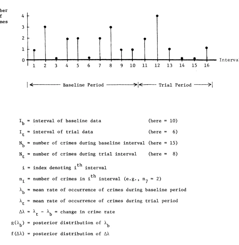
crime control program is applied (see Figure 1). During the ith interval of

observation (assume that the basic interval is a day) a total of ni crimes

are commited. The sequence {ni}, divided into baseline and trial counts,

i. the basic data input to the analysis; the output is an estimate of h(AX), the distribution of the change in crime rate.

et. Xb = crime rate during baseline period

Xt = crime rate during trial period

AX = Xt - Xb = change in crime rate

g(Xb) = posterior distribution of b

f(AX) = posterior distribution of b

In a Bayesian perspective, the crime rates Xb and AX are treated a. random variables whose different possible values are supported more or less strongly

by the crime count data. The relative credibilities of these different values

are expressed in the posterior distributions g(%b) and f(AX).

Consider the distribution f,~A). We begin by finding the distribution of

the change in crime rate AX cord4iiontal on particular value of baseline

crime rate X,, then we uncondition by integrating over the posterior

distribu-0

tion of . For any given value of Xbe the change in crime rate could be any

number reater than or equal to - : this recognizes both tcna the trial

period crin.- rate Xt = Xb + AX cannot be negative and that it might possibly

(9)

-4-Figure 1: Data and Variable Definitions

Number of 4 1 Crimes 3 2 0

I

< Baseline Period >|< Trial Period

-

>

Ib = interval of baseline data (here = 10)

It = interval of trial data (here = 6)

Nb = number of crimes during baseline interval (here = 15)

Nt = number of crimes during trial interval (here = 8)

i = index denoting ith interval

ni = number of crimes in i interval (e.g., n7 = 2)

b = mean rate of occurrence of crimes during baseline period

At = mean rate of occurrence of crimes during trial period

AX = At - Ab = change in crime rate

g(Xb) = posterior distribution of Xb

f(AX) = posterior distribution of AX

(10)

-5-which, while reducing total crime, nevertheless increases total reported crime; it is reported crimes which constitute the data base for the program evaluation. We will make the conservative choice of assuming that the

conditional prior distribution of the change in crime rate, f(AX I Xb), is

non-zero and uniform over the range - Xb < AX < . Given this (improper)

diffuse prior, the conditional posterior distribution of the change in crime rate is proportional to the conditional likelihood of observing the sequence

of counts {n Ib+l nIb+2'... nib+i _} during the trial period, generated by

a Poisson process with rate At = X_b + AX [3]:

I +I

Ib+It n

f(A I _b exp[-(Xb + AX)] (b+ A) '/n.!

i=Ib+ 1

exp[-(b + A)It](b+Ah) t - b. (1)

Thus the unconditional posterior distribution of the change in crime rate, f(AX), can be determined by integrating (1) over the possible values of baseline crime

rate b. Therefore the next task is to determine the posterior distribution of

the baseline crime rate, g(Xb).

We begin with the choice of a prior distribution. We might either choose a diffuse prior or follow suggestions in the literature [i,4] and choose a

logarithmically flat prior (i.e., a prior a bl). We opt for the anter, although

with reasonably large counts of crimes Nb in the baseline period (as in the

Nashville case) this choice makes little practical difference. Since the

(11)

-6-distribution of Xb becomes b n. g(%b) a ~ Xb H exp[-Xb] Xb /n.! i=l Nb-1 Oa exp[-XbIb] Xb Xb >O

We can now combine (1) and (2) to obtain the unconditional posterior distribution of the change in crime rate

o Nt

f(AX) a f exp[-(X_b + AX)I ]( _b + A) Lb=t(AX)

Nb-1

exp[-XbIb] Xb dXb

L(AX) = max[O,-AX] .

The integral (3) can be reduced to a simple finite sum when L(AX) = 0 but becomes

a finite sum of incomplete gamma functions when L(AX) = - AX. We will solve

(3) by numerical integration. The special case AX = 0 can be solved analytically

using the fact that

0oo f x nexp(-ax)dx = n+ n+l x=O a (N_t + Nb-l)! Thus f(0) NL) (I + I Nt+Nb_b

this value provides a useful check on the accuracy of the numerical integration. (2) where (3) (4) (5) (6)

(12)

-/-3. Application to Nashville Data

The Nashville experiment set out to determine the impact on Part I crimes (robbery, larceny, burglary, motor-vehicle theft, forcible rape,

aggravated assault and homocide) of saturating small areas with police patrol

cars. Four zones with high crime rates were selected for study. The first

two zones, referred to as "Day Patrol One" and "Day Patrol Two", each received

in turn 10 days of saturation patrol during the 9AM - 5PM shift. Then the

third and fourth zones - "Night Patrol One" and "Night Patrol Two" - each

received 10 days of saturation patrol during the 7PM - 3AM shift. Thus the

Nashville experiment consisted of four successive trials of 10 days each, two with daytime saturation and two with nighttime saturation. Crime counts were obtained in each of the four zones before, during, and after the 10 day trial

periods. Briefly, the results obtained by Schnelle et al. [1] were that no

statistically significant changes in crime rate were observed in the two day-time trials, but significant decreases were observed in both nightday-time trials.

We will re-analyze the Nashville data using the Bayesian methodology

developed above. The first step is to confirm that the data are in fact well

described by a Poisson model. On the assumption that the impacts of saturation patrol do not persist after patrol returns to normal levels, we will not

distinguish between crime data from before and after the 10 day trial periods of saturation patrol; rather, we combine these data to form the baselines. The four baseline periods range in duration from 78 to 116 days. Shown in Table 1 are the distributions of crimes per day in each of the four trials. Using the dispersion test [5], the hypothesis that the counts of crime arise

(13)

-8-TABLE 1

Comparison of Nashville Baseline Data to Poisson Model

(source: Schnelle et al. [1])

# DAYS WITH GIVEN # EVENTS (EXCLUDING SATURATION TRIAL DAYS)

"DAY PATROL 1" "DAY PATROL 2" "NIGHT PATROL 1"

"NHT PATROL ""NGHT PATROL 2

"NIGHT PATROL 2"'NIGHT PATROL 2*

0 1 2 3 4 5 6 7 Total days I_b Total crimes Nb N b Xb = I 2 _b X d.f. z 26 (26) 35 (36) 33 (36) 29 (29) 37 ('35) 42 (42) 15 (16) 15 (17) 29 (25) 4 (6) 5 (5) 11 (10) 4 (2) 2 (1) 1 (3) 0 (0+) 0 (0+) 0 (1) 0 O 0 (o+ ) 0 0 0 78 94 116 87 90 137 1.115 0.957 1.181 82.45 91.73 94.15 77 93 115 0.47 -0.06 -1.41 31 (26) 31 (28) 32 (36) 32 (36) 23 (24) 23 (24) 10 (11) 10 (10) 5 (4) 5 ( 3) 1 (1) 1 ( 1) o (o+) 0 (0+ ) 1 0 103 102 140 133 1.359 1.304 130.74 111.65 102 101 1.92 0.77 Signif. (2 tail) 0.64 0.95 0.16 0.06 0.44

Serial auto corre- 0.021 -0.013 -0.118 0.022

lation

Notes:

b (n X )2

a) X2 dispersion test Xdispersion test x 2 E b (ni x b chi square df = Ib - 1

i=l b

for large Ib refer - /21b 3 to Gaussian (0,1)

(R.L. Plackett, Analysis of Categorical Data, pg. 10).

deleting the busy day from "Night 2" is conservative if want to establish a reduction in .

Counts in parenthesis are expected Poisson counts, rounded to nearest integer. # CRIMES

(14)

-9-from a Poisson process cannot be rejected at the 0.05 level in any of the four trials. However, the second nighttime trial nearly achieves the 0.05 significance level and deserves special comment. That particular baseline is unusual in that it contains one night shift in which 7 crimes were

committed -the highest total for any single shift in the entire study. This exceptional case occurred shortly after the saturation trial and may repre-sent temporally-displaced crime, one very active criminal, or a just a typical fluctuation. If we set aside that datum (forming the fifth column in Table 1, labelled "Night Patrol 2*"), we not only make a more conservative estimate of the impact of saturation patrol but also achieve a distribution very well described by the Poisson. Testing for serial correlation in each of the four series indicates that the Poisson assumption of independence between crime counts on successive days is also valid, since the serial correlation coefficient never exceeds 0.12 in absolute value. Thus the dispersion tests and tests for serial correlation both confirm the validity of modeling the count of crimes as a

?oisson variate.

Given that the Poisson model is valid, we can use (3) to determine the shape of the distribution of the change in crime rate during saturation patrol. The results of the numerical integrations are displayed in Figure 2. As noted by Schnelle et al. [1], the nighttime saturation patrols produced a consistent and clear drop (about -0.8 crimes per shift), whereas the daytime patrols give neither clear nor a consistent indication of impact.

When interpreting these results for substantive purposes, one must be

aware of two potential pitfalls. The first is a possible change in the crime

report-ing behavior of the public. It has been observed in other studies [6] that increas-ing police presence can lead to an increase in the fraction of crimes reported

(15)

-10-Figure 2

Posterior Distribution of Change in Crime Rate AX = Xt - Xb

1 t b 4J 44 a a ) a a) U) w E Y JJ v 0 a) .-4 Cd -W

I-~cdu

_s _{X U}

C!$C

9-4 To Lf, n_. o0 I I 0 0 .H -i (U *14 a) -h . X p 4 V wc~

(16)

-11-to police. This problem may not be too serious in the Nashville study, since

saturation trials lasted only ten days and since Schnelle et al. found that crimes were almost never reported directly to patrolling officers during

either the baseline or trial periods. The second potential pitfall is spatio-temporal displacement of crime, which may be a more serious issue in the

Nashville case. Since the trials were so brief, some crime may have merely

been delayed, rather than permanently averted. Schnelle et al. were careful

to check for spatial displacement of crime, but one wonders whether their test

was sufficiently sensitive. Since the drop in crime rate amounts to roughly

1 crime per shift and since there are 33 patrol zones in Nashville, it would be quite possible for the one crime to be displaced and not detected. Even looking at only those zones contiguous to the experimental zones, a displacement of such a small number of crimes would still be hard to detect if the crimes were displaced to a different contiguous zone each night. While our main pur-pose in this paper is to develop the Bayesian methodology rather than to address

the substantive question, and while Schnelle et al. took care to check for dis-placement, we should be aware of possible problems in interpretation of results

(17)

-12-4, Methodology for Ratio of Crime Rates

Section 2 of this paper developed a methodology for estimating the

difference in the crime rates during the baseline and trial periods. In

this section we outline an alternative which expresses the experimental impact as a proportionate reduction (or increase) in the crime rate. Our goal is to estimate the ratio of crime rates

R = Xt/Ab (7)

As before, we assume that the crime count in each period is a Poisson variate. We note that non-Bayesian methods are available for this problem [7] but again

prefer the distributional form of results provided by the Bayesian approach. Values of R less than unity indicate successful crime-reduction programs;

the relative credibility of various estimates of R will be readily grasped in the Bayesian framework.

Our approach again is to find the posterior distribution of R conditional on the value of Xbs then uncondition by integrating over the posterior

distri-bution of b given the baseline data. As before, we will take this posterior

distribution of b to be a gamma distribution

N -l

g(Xb) a exp(- XbIb) Xb xb > 0. (8)

Of particular interest is the choice of prior distribution for R

condi-tional on the value of Xb. If we expected that the experimental program would

definitely reduce the crime rate, we might use a beta distribution for

O < R < 1.0. To allow for the possibility that R > 1.0, we can use a gamma

(18)

-13-from the value of b; it is difficult to imagine a compelling, systematic

way to link the value of R with the value of X_b. If one prefers a diffuse

prior, one can set A = B = 0. If one wants a roughly bell-shaped prior with mean R and standard deviation R' one should choose the integer values

closest to

A = (R/o)2 -1

B = /(R )

With the gamma prior distribution for R, the conditional posterior distribution Ib+It exp[-RXb](RXb) 1 f(RIXb) a Ib i=I +1 b RA exp [-BR] n.! 1 N exp(-RXbI_t)(Rb)t RA exp [-BR] .

Unconditioning using (8) we find

oo A+N f(R) a f R Xb=0 N exp[-BR] b Nb-1 exp[-RItXb] Xb exp[-XbIb] dXb oo Nt+Nb-1 t b b exp[-(RIt+Ib)Xb] db (N_t + Nb-l)! t b (RI t + Ib)Nt+Nb .... - (Nt+Nb) exp l-bK] LKit t lb] (9) (10) (11) (12) A+N a R t exp [-BR] (13) A+N Oa R exp [-BR] (14) A+N R r f(R) a (16)

(19)

In the case of a diffuse prior, (16) specializes to

N -(Nt+N_{b )}

f(R) a R [RI_t + Ib] (17)

The Nashville data have been analyzed using (17); results are shown in Figure 3. As in Figure 2, the nighttime patrols were clearly successful, whereas the daytime results are weak and mixed.

(20)

-15-Posterior Distribution o

Figure 3

f Proportional Reduction in Crime Rate

C14 P4 0 H IP4 -IC HO ZP4 II H EH H ¢ Z O .4 - *Hl 4i _cn 44 _u, o $-4 -W W H 1n 0 H.-R = t/Xb o . 0 O H o 4 O 0 0 H r-d C" o Ln 0 _O w

(21)

-16-References

1. J.F. Schnelle, R.E. Kirchner, J.D. Casey, P.H. Uselton, and M.P.McNees,

"Patrol Evaluation Research: A Multiple Baseline Analysis of Saturation

Police Patrolling During Day and Night Hours", Journal of Applied Behavior Analysis, Vol. 10, No. 1, 1977, pp. 33-40.

2. A.F.S. Lee and S.M. Heghinian, "A Shift in the Mean Level in a Sequence

of Independent Normal Random Variables - A Bayesian Approach", Technometrics, Vol. 19, No. 4, November 1977, pp. 503-506.

3. S. Schmitt, Measuring Uncertainty: An Elementary Introduction to Bayesian

Statistics (Addison-Wesley, Reading Mass., 1969).

4. C. Villegas, "On the Representation of Ignorance", Journal of the American Statistical Association, Vol. 72, No. 359, September 1977, pp. 651-654. 5. R.L. Plackett, The Analysis of Categorical Data (Griffin: London, 1974). 6. S. G. Chapman, Police Patrol Readings (Charles C Thomas, Springfield, Ill.,

1972), pp. 342-352.

7. D.R. Cox and P.A.W. Lewis, The Statistical Analysis of Series of Events (Methuen: London, 1966).