Recursive decomposition tree of a Moore co-family and closure algorithm

HAL Id: hal-02024930

https://hal.archives-ouvertes.fr/hal-02024930

Submitted on 19 Feb 2019

HAL is a multi-disciplinary open access

archive for the deposit and dissemination of

sci-entific research documents, whether they are

pub-lished or not. The documents may come from

teaching and research institutions in France or

abroad, or from public or private research centers.

L’archive ouverte pluridisciplinaire HAL, est

destinée au dépôt et à la diffusion de documents

scientifiques de niveau recherche, publiés ou non,

émanant des établissements d’enseignement et de

recherche français ou étrangers, des laboratoires

publics ou privés.

Recursive decomposition tree of a Moore co-family and

closure algorithm

Pierre Colomb, Alexis Irlande, Olivier Raynaud, Yoan Renaud

To cite this version:

Pierre Colomb, Alexis Irlande, Olivier Raynaud, Yoan Renaud. Recursive decomposition tree of a

Moore co-family and closure algorithm. Annals of Mathematics and Artificial Intelligence, Springer

Verlag, 2014, 70 (1-2), pp.107-122. �10.1007/s10472-013-9362-x�. �hal-02024930�

(will be inserted by the editor)

Recursive decomposition tree of a Moore co-family

and closure algorithm

Pierre Colomb · Alexis Irlande · Olivier Raynaud · Yoan Renaud

Received: date / Accepted: date

Abstract A collection of sets on a ground set Un (Un ={1, 2, ..., n}) closed

under intersection and containingUn is known as a Moore family. The set of

Moore families for a fixed n is in bijection with the set of Moore co-families (union-closed families containing the empty set) denotedMn. This paper

fol-lows the work initiated in [9] in which we have given an inductive definition of the lattice of Moore co-families. In the present paper we use this definition to define a recursive decomposition tree of any Moore co-family and we design an original algorithm to compute the closure under union of any family. Then we compare performance of this algorithm to performance of Ganter’s algorithm and Norris’ algorithm.

Keywords Closure systems_{· Enumeration algorithm · Lattice theory}

Pierre Colomb

Clermont University, University Blaise Pascal, Campus des Cézeaux 63173 Clermont-Ferrand, France

E-mail: [email protected] Alexis Irlande

Universidad Nacional de Colombia Bogotá, Colombia E-mail: [email protected]

Olivier Raynaud

Clermont University, University Blaise Pascal, Campus des Cézeaux 63173 Clermont-Ferrand, France

E-mail: [email protected] Yoan Renaud

INSA de Lyon, Bâtiment Blaise Pascal, Campus de la Doua, 69621 Villeurbanne, France E-mail: [email protected]

1 Introduction

The concept of a collection of sets closed under intersection appears with dif-ferent names depending on the scientific fields. The name Moore family was first used by Birkhoff in [4] referring to E.H. Moore’s research. But, very fre-quently, such a collection on a ground set Un (Un = {1, 2, ..., n}) is called

closure system. This concept is applied to numerous fields in pure or applied mathematics and computer science. For instance Cohn, Sierksma and van de Vel have used it in the framework of algebra and topology ([10, 23, 24]) while Birkhoff, Davey and Priestley focused on order and lattice theory ([3, 14]). Formally a closure operator is an extensive, isotone and idempotent function on 2Un _{(the set of all subsets of U}

n), and a closure system is then the set

of its fixed points. In particular, it is well-known that any closure system is a complete lattice. In 1937, Birkhoff ([3]) gave a compact representation of quasi-ordinal spaces (in other words, collections of sets closed under inter-section and union and so which are distributive lattices). More recently the notion of closure system appears as a significant concept in computer science with research in relational databases ([12]), data analysis and formal concept analysis ([16, 1, 17]). More precisely, Ganter and Wille defined a mathemati-cal framework for classification, and Barbut defined and used Galois lattices about questions raised in Guttman scales analysis ([1]). Meanwhile, in 1985, equivalent collections of sets were called knowledge spaces by Doignon and Falmagne ([11]). In that context, a set of the collection is a possible state of knowledge of a student following a specific discipline in an educational setting and such that each element of the state is some elementary fact or question known by the student. The hypothesis is that the union of any set of states is itself a knowledge state.

An important fact is that the collection of Moore families on Un is itself a

closure system. Indeed, the system composed of Moore families onUncontains

a maximum element (2Un_{) and the intersection of two Moore families is a}

Moore family itself. To get an overall view of the properties of this closure system, see the survey [7]. There exists a one-to-one mapping1 between the set of Moore families and the set of Moore co-families defined dually as the set of union-closed collections of subsets ofUn containing the empty set. The

latter is denoted byMn.

Some researches focus on quantitative properties of this lattice of Moore co-families. As an example, Demetrovicset al. in [15] noticed that the problem of counting Moore co-families onn elements is a complex issue for which there is no known formula. Even the lack of such a formula has not been proved. In [6], Buroshet al. consider the issue of counting Moore families as natural, so they provide an upper bound for that number (see also [13]). An often supported approach to try to obtain such a formula involves counting the number of

1 _{Basically, for a given Moore family, one only has to complement every set to obtain a}

Moore co-family. For example, the Moore family {{1}, {1, 2}, {1, 3}, {1, 2, 3}} on U3

objects for the first values of n using a systematic procedure. In [20], Habib and Nourine computed this number forn = 6 and in [8], Colomb et al. found 1019_{families forn = 7. We can find such integer sequences on the well-known}

On-line Encyclopedia of Integer Sequences2.

From this quantitative study of the lattice, the same authors were able to state an inductive definition of the lattice (see [9]). In the present paper we de-fine a recursive decomposition tree of a Moore co-family and then we design an original algorithm to compute the closure of any given family. Then we com-pare the performance of this algorithm to performance of Ganter’s algorithm and Norris’ algorithm. The paper proceeds as follows. Section2 introduces the inductive definition of the lattice of Moore co-families. Section3 describes how each Moore co-family can be represented by a decomposition tree relying on the inductive definition (see Theorem 1). In section 4 we introduce the new algorithm and we give practical performance in section5.

In the rest of the paper, we denote elements by numbers (1, 2, 3, . . . ). Sets are denoted by capital letters (A, B, C, . . . ). Families of sets are denoted by calligraphic letters (_{A, B, C, . . . ). Finally, we denote the sets of families of sets} by black board letters (A, B, C, . . . ).

2 Inductive definition of the lattice of Moore co-families

As explained in the introduction, the set of Moore co-familiesMn on a ground

set Un = {1, 2, ..., n} has a lattice structure. We give an example of such a

lattice with the set of Moore co-families onU2 in Figure 1. In this section we

will show how to define the latticeMn+1 from the latticeMn (see [9] and [2]

for a complete study).

{} {{},{1}} {{}, {2}} {{}, {1}, {2}, {1,2}} {{}, {2}, {1,2}} {{}, {1}, {1,2}} {{}, {1,2}}

Fig. 1 The Hasse diagram of the complete set_M2of Moore co-families on the ground set U2,

ordered by inclusion. There are exactly 7 Moore co-families on U2. This ordered set (M2, ⊆)

(orM2 for short) has a maximal element 2U2(all subsets of U2) and the intersection of two

Moore co-families is a Moore co-family. Thus,M2 admits a complete lattice structure.

2.1 Definitions and notations

For any integern_{≥ 1, let U}n denote the set{1, . . . , n}. Let M be a family on

Un, we denote (M, ⊆) the corresponding ordered set. Two sets M, M0 in M

such that neitherM _{⊆ M}0 _norM0 _{⊆ M are said incomparable in (M, ⊆). A}

family where every pair of sets is incomparable is called an antichain. We say that M is covered by M0 _{in (M, ⊆), denoted M ≺ M}0_{, if M ⊂ M}0 _{and there}

is noM00_{∈ M such that M ⊂ M}00_andM00_{⊂ M}0_{. In the following, depending}

of the context, we will denote _{M the ordered set (M, ⊆) when no confusion} is possible.

Given a family _{M, a subfamily I of M is an ideal of M if it satisfies the} following implication for any pairM , M0 in _M,

M ⊆ M0 _andM0 _{∈ I ⇒ M ∈ I.}

In other words, an ideal of_{M is some antichain of M and everything below it.} We shall useI_Mto denote the sets of ideals on_{M. Given a set X in a family} M, there exists a unique ideal I of M with X as a maximum set (also called the principal ideal generated by X inM). Let IM(X) denote this ideal. By

extension, we denoteI_Mn(M) the principal ideal generated by M in the lattice Mn. This way, IMn(M) corresponds to the set of Moore co-families included

in_M.

2.2 Compatible families

A Moore co-family _{M on U}n+1 can be decomposed into 2 parts. The part

consisting of the sets of_{M containing the element n + 1 (denoted by M}upfor

the upper part), and the complementary part (denoted by_Mlow for the lower

part). The empty set is duplicated to be present in the two parts. Naturally, M = Mup∪ Mlow. On the one hand, the family Mlow is clearly a family of

Mn. On the other hand, the familyMupis a Moore co-family onUn+1with the

peculiarity that all its sets contain the elementn + 1 (we will denoteMupn+1as

the set of Moore co-families having this property). Thus, any Moore co-family inMup_n+1can be seen as a Moore co-family inMn for which the elementn + 1

has been added to each set.

Example: Let_{M be a Moore co-family on U}3:

M = {∅, {1}, {1, 2}, {1, 3}, {2, 3}, {1, 2, 3}} We can decompose this family into two sub Moore co-families:

Mlow={∅, {1}, {1, 2}} and Mup={∅, {1, 3}, {2, 3}, {1, 2, 3}}

To study the matching conditions between a family inMn and a family in

Mup

n+1in order for their union to be a family inMn+1, we define the notion of

compatible family. Thus, we will say that a family inMn is compatible with a

∅ {1, 2, 3} {1, 3} {2, 3} ! ! ∅ {1} {1, 2} ∅ {1} ∅ {1, 2, 3} {1, 3} {2, 3} {1} ∅ {1, 2, 3} {1, 3} {2, 3} {1} {1, 2}

M

M

M

Fig. 2 On the left, a Moore co-family in_Mup₃ (all its non empty sets contain the element 3) and two different compatible Moore co-families on U2. In both cases, the obtained family,

on the right, is itself a Moore co-family.

example in Figure 2 illustrates that for a fixed upper part, there are several compatible lower parts.

In [8] we showed that for a given upper family_Mup inMupn+1, there exists

a unique compatible maximal family and that the set of compatible families with _Mup corresponds to the set of the Moore co-families contained in this

maximal family. Function fn defined hereafter is a characterization of the

maximal compatible family of a given Moore co-family inMup_n+1.

Definition 1 Letfn be a function fromMupn+1to Mn such that:

fn(M) = {X ∈ 2Un | ∀M ∈ M \ ∅, M ∪ X ∈ M}

We will write f instead of fn when no confusion is possible.

Proposition 1 [8]

Let _Mup be a Moore co-family in Mupn+1, for any Moore co-family Mlow in

Mn, the two following assertions are equivalent:

(i) _Mlow is compatible with Mup;

(ii) _Mlow ⊆ fn(Mup).

For example, the maximal family associated with _Mup (cf. Figure 2) is the

family_{{∅, {1}, {2}, {1, 2}}. Basically, it can be verified that the two compatible} families called_Mlow and given in Figure 2 are sub-families of this family.

Corollary 1 Let _Mup be a Moore co-family in Mupn+1, the set of Moore

co-families compatible with_Mup isIMn(f (Mup)).

2.3 Recursive decomposition theorem

Basically, the set Mup_n+1 can be partitioned into 2 sets: families that do not contain the singleton_{{n + 1} and families that contain it. These two sets are} in natural bijection withMn.

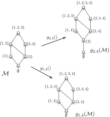
Definition 2 For any integern such that n_{≥ 1, we define} g1,n+1:Mn −→ Mupn+1

M 7−→ {X ∈ 2Un+1 _{| ∃M ∈ M \ {∅} such that X = M ∪ {n + 1}} ∪ {∅},}

g2,n+1:Mn −→ Mupn+1

M 7−→ {X ∈ 2Un+1 | ∃M ∈ M such that X = M ∪ {n + 1}} ∪ {∅},

We give an illustration in Figure 3.

∅ {2} {2, 3} {1} {1, 2} {1, 2, 3}

M

g

(

M)

g

(

M)

Fig. 3 On the left, a Moore co-family on U3. At the bottom-right, its image inMup₄ by

g1,4. One can check that all its sets contain the element 4. Singleton {4} does not belong to

Now, from a given Moore co-family _{M in M}n we can generate two sets of

Moore co-families inMn+1.

1. The set of Moore co-families which do not contain the singleton _{{n + 1}.} These families will be under the form g1,n+1(M) ∪ M0 with M0 a

com-patible Moore co-family ofg1,n+1(M). In other words M0 has to be a sub

Moore co-family of fn(g1,n+1(M)). For the convenience of the study, we

denotehnthe function fromMntoMnsuch thathn(M) = fn(g1,n+1(M)).

By this way the set of compatible Moore co-families withg1,n+1(M) is

ex-actlyI_Mn(hn(M)).

2. The set of Moore co-families which contain the singleton _{{n + 1}. These} families will be under the form g2,n+1(M) ∪ M0 with M0 a compatible

Moore co-family ofg2,n+1(M). In other words M0 has to be a sub Moore

co-family offn(g2,n+1(M)). But one can check that fn(g2,n+1(M)) is equal

to _{M. For this reason, the set of compatible families with g}2,n+1(M) is

exactly I_Mn(_M).

An illustration is given in figure 4.I_Mn(hn(M)) (respectively IMn(M)) is the

principal ideal generated byhn(M) (respectively M) in the lattice Mn.

M

M

Fig. 4 On the left, the lattice Mn of the Moore co-families on Un. On the right, both

isomorphic images of this lattice obtained by functions g1,n+1and g2,n+1. The gathering of

Theorem 1 states that the set of Moore co-families onUn+1can be obtained

from the set of Moore co-families onUn. In the recursive decomposition formula

given below forMn+1, we use the functionsg1,n+1,g2,n+1andhndefined above.

Theorem 1 (Colomb etal.[9]) For any integer n such that n≥ 1, Mn+1= _SS_M∈Mn{g1,n+1(M) ∪ M0 | M0∈ IMn(hn(M))} ∪

M∈Mn{g2,n+1(M) ∪ M

00 _{| M}00_{∈ I}

Mn(M)}

In other words, there exists a natural bi-partition ofMn+1: the families not

containing the singleton_{{n + 1}, under the form g}1,n+1(M) ∪ M0 withM0 as

a sub Moore co-family ofhn(M) and the families containing {n + 1}, under

the formg2(M) ∪ M00 withM00as a sub Moore co-family ofM.

3 Recursive decomposition tree of a Moore co-family

3.1 Definition

Let_{M be a Moore co-family in M}n andx be in Un, we denoteMx(resp.Mx¯)

the restriction of_{M to its sets containing x (resp. to its sets not containing} x). The empty set is added toMx.

3.2 Theoretical results

Another interpretation of the inductive definition ofMnstated by Theorem 1 is

that any Moore co-family can be decomposed by a recursive process described by Corollary 2.

Corollary 2 Let_{M be a Moore co-family in M}n, for any elementx in Un,M

can be written_Mx¯∪ gi,x(M0) withM0 such thatgi,x(M0) corresponds toMx.

This way,_{M is decomposed in two Moore co-families M}¯xand M0. Applying

recursively this decomposition principle we obtain a decomposition binary tree of_{M (each leaf is an empty set which cannot be further decomposed). The left} branch of a node _{M, labelled ¯x, leads to M}x¯ and the right one, labelledgi,x,

leads to _M0 such that gi,x(M0) is equal to Mx (if the singleton{x} ∈ M we

havei = 2, if not i = 1).

An example of decomposition of a Moore co-family is given in Figure 5. Basically each leaf of the tree shall relate to one set, and only one, of the initial family _{M. To obtain the set corresponding to a leaf, one just has to} iteratively apply the different functions g1,x org2,x that can be found in the

{3,123,35,1235} {ø,12,5,125} {ø, 3, 34, 123, 1234, 35, 345, 1235, 12345} g1,4 g2,3 g2,5 {ø,3,123,35,1235} {ø} 4 {ø,12} {ø} {1,15} {ø,12,5,125} g1,2 {ø,5} g2,1 {ø,5} {2} g1,1 g2,2 {ø} g2,3 3 2 1 5 3 1235 34 1234 ø 5 {ø} g2,5 {ø} 35 {ø} {ø,12} {2} g1,1 g2,2 {ø} 1 345 12345 5 {ø} g2,5 {ø} 123 M¯_{4 M}! M = M¯4∪ g1,4(M!)

Fig. 5 Decomposition of a Moore co-family. The family M0only owns a right branch.

3.3 Proper decomposition tree

As we can see on the example given in Figure 5, some nodes only own a right branch. This may occur in two well-defined cases: either when the chosen elementx belongs to each sets of the family, or when the family is reduced to only one set to be further decomposed.

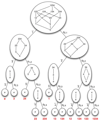
However, it is always possible to obtain a proper binary tree (i.e. a tree with the property that any internal node owns exactly two sons, also called full binary tree). Indeed, in the first case, for any given family with at least two sets, there exists always an element x which belongs to a set and does not belong to another one. By choosing this element wisely we are ensured that the node will have a left branch and a right one. The second case can be detected and the recursive process easily adapted. In Figure 6, we give a proper decomposition tree for another family.

Remark: It is well known that in a proper binary tree the number of leaves is equal to the number of internal nodes plus one. This point will be further addressed to state the time complexity of the closure algorithm.

1234 234 123 134 24 23 13 12 3 1 ø 234 24 23 3 ø 3 ø ø ø 34 4 3 4 4 ø ø ø 234 23 34 3 2 ø 34 3 ø 34 3 ø ø 4 ø 4 ø ø ø ø ø 1 2 3 2 3 3 3 g1,2 g2,2 g2,1 g2,3 g2,4 g2,4 g2,4 4 4 4 g2,3 _{g2,3 g2,3} ø 3 24 23 234 1 13 134 123 1234 124 24 4 4 ø ø ø g2,4 4 12 124

Fig. 6 Proper decomposition tree of a Moore co-family. Each internal node of the tree owns two sons.

4 Algorithm to compute the union closure of a family

Problem of generation of closed-sets from a given family has been well-studied these last years. Most of existing algorithms are based on a decomposition strategy [18, 5, 21, 19]. As previously stated, generation of closed-sets and co-closed sets can be treated in the same way (i.e. one only have to complement every sets of input and output families to obtain both closed and co-closed families). In this section, we present an algorithm to generate a Moore co-family_{M from its set of join-irreducible elements denoted JM}. This way, this algorithm can be used to compute the closure by union of any given family. This algorithm is based on Theorem 1.

4.1 Definition

A set J ∈ M is called a join-irreducible of M if J covers only one set in M. The set of all join-irreducible sets of M is denoted JM. By extension,

we denote by (_JM)x (resp.(JM)x¯) the set of join-irreducible elements ofM

which contains the elementx (resp. which do not contain the element x). We call union product between two families_M1andM2, denotedM1⊗ M2, the

set_{M1∪ M2 | M1∈ M1, M2∈ M2}.

4.2 Theoretical results

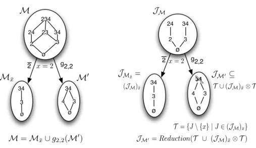
We propose an algorithm based on the decomposition of a Moore co-family that only uses families of join-irreducible sets. In other words, for each step of the recursive decomposition, given a local set _JM, we compute families of sets _JM¯x and_JM0 corresponding to the join-irreducible sets of M¯xand M0

such that_{M = M}x¯∪ gi(M0) (see Figure 7). Leaves of the decomposition tree

obtained after the whole recursive decomposition correspond to the closure of the family_{M (see Figure 8).}

Proposition 2 Let _{M, M}0 _{∈ M}n, let x ∈ Un and let i ∈ {1, 2} such that

M = Mx¯∪ gi,x(M0). Then

– _JM¯x= (_JM)x¯;

– _JM0 ⊆ {J\{x} | J ∈ (J_M)x} ∪ ((JM)x¯⊗ {J\{x} | J ∈ (JM)x}).

An illustration is given in Figure 7. Proof

– _JM¯x= (JM)x¯

Any join-irreducible element of_{M not containing x is also join-irreducible} of _Mx¯. Indeed, all the predecessors of each set in M not containing x,

don’t containx itself. Similarly, there is no new join-irreducible element in JM¯x.

– _JM0 ⊆ {J\{x} | J ∈ (J_M)x} ∪ ((JM)x¯⊗ {J\{x} | J ∈ (JM)x})

Let us show that gi,x(JM0) ⊆ (J_M)x ∪ ((JM)x ⊗ (JM)¯x). Let J ∈

gi,x(JM0), then J∈ J_Mx. Two cases occur:

– J _{∈ JM} and withx_{∈ J we obtain J ∈ (JM})x;

– J owns one, and only one, immediate predecessor in_Mx and another

one, and only one, in _Mx¯. By contradiction, let us suppose by

hy-pothesis that J _{6∈ (JM})x ⊗ (JM)x¯. Let S = {s1, s2, ..., sn} (resp.

S0 _{= {s}0

1, s02, ..., s0m}) be the family of maximal join-irreducible sets

of _M¯x (resp. of Mx) such that ∀i, si ⊂ J (resp. ∀j, s0j ⊂ J). Let

M ax = max(S_{⊗ S}0_{), we have M ax ⊆ M}

x and by hypothesis we

have _{∀m ∈ Max, m 6= J and so |Max| > 1. With J = (}S_m∈Maxm) we conclude that J _{6∈ J}Mx. J\ {x} 6∈ JM0 and then J 6∈ gi,x(JM0).

u t 234 23 34 3 2 ø 34 3 ø 34 3 ø 2 g2,2 24 4 34 3 2 34 3 2 g2,2 ø ø 3 ø 24 4

J

=

M

M

J

M

J

⊆

M = M

∪ g

(

M

)

Fig. 7 On the left, M is splitted in two parts according to theorem 1 with x = 2. Singleton {2} belongs to M and so i = 2. We have M = Mx¯∪ g2,2(M0). To compute the closure of a

given family, we will simulate this step by the process illustrated on the right of the figure. From the set of join irreducible elements of M denoted JM, thanks to Proposition 2 we

compute the set JM¯xof join-irreducible elements of Mx¯ (on the left branch), and the set JM0 of join-irreducible elements of M0(on the right branch). The set {3, 4}, in bold, is not a join-irreducible element and it will be deleted by the reduction step.

Proposition 2 gives an exact characterization of the set _JM¯x and merely

states a superset of_JM0. But setsJ_M0 and{J\{x} | J ∈ (J_M)x} ∪ (JM)x¯⊗

{J\{x} | J ∈ (JM)x} share exactly the same set of join-irreducible elements.

Thus, it will be enough to proceed to a step of reduction to obtain the exact value of_JM0. We call process of reduction of a family, the process consisting

of deleting all non join-irreducible sets of the family.

4.3 Algorithm

The given Algorithm 1 is recursive and the stop case arises when the local family_JF is reduced to one set.

In the general case, an element x is wisely chosen (see Section 4.5) and the algorithm computes the set of join-irreducible elements of _Fx¯ and of F0

launched on the left branch with (_JF)x¯ as input family. After that, the set

JF0 is computed thanks to a reduction process from the set {J\{x} | J ∈

(JF)x} ∪ (JF)x¯⊗{J\{x} | J ∈ (JF)x}. The recursive process is then launched

again, corresponding to the right branch, and the element x is added to the current solution. See Figure 8 for an example.

Note: It is important to understand that the algorithm operates well even if the given family is not reduced (the call to the reduction process in Line4, Algorithm 1, is optional). Although the process of reduction is the opposite process to the closure process, our experimental results have shown that it was much more efficient to reduce the given family before proceeding with the closure process.

Algorithm 1: Co-closure(_JF,S) Input:_JF a family of sets;

S the initial part of the current solution; begin if _JF =_{{E} then} print(E∪ S); else 1 Choose an elementx inS_JF\T_JF; 2 J_Fx¯ ← {E | x 6∈ E, E ∈ J_F}; 3 T ← {E \ {x} | x ∈ E, E ∈ J_F}; Co-Closure(_JFx¯, S); 4 J_F0 ← Reduction(T ∪ J_Fx¯⊗ T ); Co-Closure(_JF0,S∪ {x});

4.4 Discussion about the time complexity of Algorithm 1

We denote_{|Co − closure(F)| the size of the closure under union of the family} F. Since the decomposition tree obtained at the end of the whole process of Algorithm 1 is a proper binary tree, we know that this tree owns exactly |Co − closure(F)| − 1 internal nodes3_{. This means that the time complexity}

needed to compute one set of the closure corresponds exactly to the time complexity needed to treat one internal node. Moreover in the following we will suppose that the size of the ground set Un is constant. This way, the

operations on sets like intersection and union will be considered feasible in constant time.

Let_{F be the local family of an internal node. Lines 1, 2 and 3 of Algorithm} 1 can be treated in one pass through the family_{F. All these operations can}

3 _{For any proper binary tree, the number of leaves is equal to the number of internal}

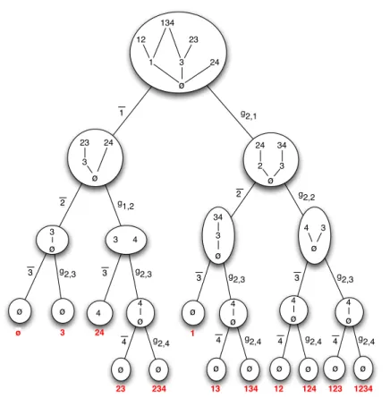
24 23 3 3 4 3 4 4 34 3 2 34 3 4 4 1 2 3 2 3 3 3 g1,2 g2,2 g2,1 g2,3 g2,4 g2,4 g2,4 4 4 4 g2,3 _{g2,3 g2,3} ø 3 134 24 23 12 3 1 ø ø ø ø ø ø ø ø ø ø ø ø ø ø ø ø ø 3 ø 24 23 234 1 13 134 123 1234 24 4 g2,4 4 ø ø ø 12 124 4

Fig. 8 Proper decomposition tree obtained by the execution of Algorithm 1 on the set of join irreducible elements of the family given in Figure 6. One can check that leaves of the trees are strictly identical.

be done in _{O(|F|). Basically, the whole complexity of the computing lies in} line 4 with two processes: a process of union product between two sets and then a process of reduction of the obtained family. These two processes are quadratic in the size of the involved families. The most noteworthy fact is that sizes of this families are not always polynomially correlated with the size of the initial family (we mean the family of the root of the tree). But one has to know that the size of the family resulting of the product is never greater than to the number of leaves of the sub-tree rooted in this internal node. This means that the local time complexity is polynomially linked with the size of the sub-result rooted in this node.

4.5 Discussion about the choice of the elementx

The choice of the elementx leads to a bi-partition of the input family_JF into

JF¯x and T (see Lines 2 and 3, Algorithm 1). Thus the sum |JFx¯| + |T | is

a process of union product between_JFx¯ andT and a process of reduction of

the result. These two operations have a time complexity in_O(|JFx¯| ∗ |T |).

– Regarding the union product, the biggest complexity comes when sets have approximately the same size. By this way, we must choosex to ensure that |JFx¯| or |T | is minimum.

– Our experimental studies show that the majority of time is spent on the process of reduction. Along the left branch of the recursive process, the time consuming process steps such as the reduction is the sum of the times spent on the reduction of each set _{T . The complexity of this reduction} being quadratic, to achieve short response times, the smallest possible sub-families which do not contain x should always be used.

For these two reasons, the best choice for x is the element which occurs the least often. But it is, in any case, essential to state here that, in spite of all these general rules, the computation time to find x will increase significantly calculation times of the whole process.

5 Experimental results

5.1 Experimental design

In order to assess performance, the approach described previously has been implemented in C. The executable file was generated with compiler GCC 4.4. The experiments were performed on a AMD Opteron 8356 processor with 2.3 GHz of speed and 256 Go of memory. Several well-known benchmark real-world data-sets were chosen from UCI4_{. The following table summarizes the}

data-sets characteristics.

Table 1 Data-sets characteristics of several well-known benchmark data-sets chosen from UCI.

Data-sets # Attributes # Sets # Attributes per set # Closed set Mushroom 119 8124 23 238 709 Chess 75 3196 37 930 851 336 Connect 129 67557 43 1 415 737 994

To compare performance of Co-closure and previous approaches with re-spect to the size of family, we implemented a version of Norris’ algorithm (see [22]) as well as a version of Ganter’s algorithm called Next-closure (see [18]). It can be noticed that we have used the natural one to one mapping be-tween Moore and co-Moore families to compute closed sets using Co-Closure algorithm.

5.2 Result

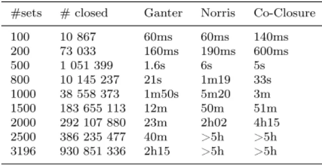
We have compared execution time of these different algorithms on parts of benchmark data-sets. In that way, we have run algorithms on the firstm sets of each benchmark data-sets by varying m. On Tables 2, 3, and 4 we give numbers of co-closed sets we obtained by execution of the three algorithms for each size of the considered data-sets partition. In the last three rows we give the execution time for each algorithm.ms stands for milliseconds, m for minutes,h for hours and d for days.

Table 2 Chess

#sets # closed Ganter Norris Co-Closure 100 10 867 60ms 60ms 140ms 200 73 033 160ms 190ms 600ms 500 1 051 399 1.6s 6s 5s 800 10 145 237 21s 1m19 33s 1000 38 558 373 1m50s 5m20 3m 1500 183 655 113 12m 50m 51m 2000 292 107 880 23m 2h02 4h15 2500 386 235 477 40m >5h >5h 3196 930 851 336 2h15 >5h >5h Table 3 Mushroom

#sets # closed Ganter Norris Co-Closure 50 1208 75ms 75ms 90ms 100 3459 80ms 85ms 150ms 200 7086 80ms 95ms 310ms 500 17 781 120ms 180ms 570ms 1000 32 513 205ms 380ms 900ms 1500 48 414 340ms 680ms 1.5s 2000 58 982 430ms 1s 1.7s 2500 72 008 490ms 2s 2.5s 3000 80901 700ms 2.1s 3s 4000 104 104 1s 3.5s 4.5s 5000 136 401 1.5s 5s 7s 6000 156 573 2s 7.5s 8.5s 7000 214 950 3.5s 11.7s 13s 8000 237 874 4s 17s 15s 8124 238 709 4.1s 17.4s 15.5s

Table 4 Connect

#sets # closed Ganter Norris Co-Closure 100 13 406 730ms 760ms 850ms 200 63 360 840ms 900ms 1.3s 300 149 393 875ms 1.2s 2s 500 445 676 1.3s 3.1s 7.3s 800 753 371 2s 8s 14s 1000 1 069 569 3s 17s 24s 2000 4 732 622 20s 2m 3m40s 3000 9 742 932 1m 5m35s 20m 5000 22 543 073 3m25s 26m 3h15m 10000 69 916 189 20m >4h >5h 20000 242 644 240 2h30 >4h >5h 67557 1 415 737 994 4d >4h >5h

5.3 Analysis of the results

The first point to note here is that Ganter’s algorithm shows the best perfor-mance in each context. Basically, the perforperfor-mance of the proposed algorithm appears to be equivalent to the performance of Norris’ algorithm. We should add that in some cases this algorithm exceeds Norris’. Moreover, let us recall that Norris’ algorithm consumes a lot of memory. Indeed the family resulting of the computing is kept in memory during all the process. Note that it is not the case of the algorithmic process described in this paper.

6 Conclusion

In [8] authors have computed the exact size of_|M7|. From this first technical

challenge has derived a recursive decomposition theorem which has been for-malized in [9]. In the present article we have shown that each Moore co-family can be represented by a proper decomposition tree and we use this principle to design an original algorithm to close by union any family. The process has been implemented and the results on well-known benchmarks are given in the last section. Experimentations state the correctness of the process but show that time complexity is not satisfying. However, we think this straightforward process is interesting by itself. Moreover we have determined two major ways of improvement :

– Since most of the time is spent on the reduction of the set of join-irreducible elements on the right branch, a question could be to early detect sets, produced by a union product, which will not be join-irreducible elements and so will be deleted by the reduction process.

– A second interesting question will be the design of some kind of dynamic programming algorithm to take into account the redundancy of families which appear in the bottom part of the tree. Maybe we should use another closure algorithm in this part of the process.

References

1. Barbut, M., Monjardet, B., Ordre et classification. Hachette (1970)

2. Beaudou, L., Colomb, P., Raynaud, O., Structural properties and algorithms on the lattice of Moore co-families. In proceedings of ICFCA (Supplementary actes), p.41–52 (2012)

3. Birkhoff, G., Rings of sets. Duke Mathematical Journal 3, p.443–454 (1937) 4. Birkhoff, G., Lattice Theory. Third edn. American Mathematical Society (1967) 5. Bordat, J.P., Calcul pratique du treillis de galois d’une correspondance. Math. Sci. Hum.

96, p.31–47 (1986)

6. Burosh, G., Demetrovics, J., Katona, G., Kleitman, D., Sapozhenko, A., On the number of databases and closure operations. Theoretical computer science 78, p.377–381 (1991) 7. Caspard, N., Monjardet, B., The lattices of closure systems, closure operators, and

impli-cational systems on a finite set: a survey. Discrete Applied Mathematics 127, p.241–269 (2003)

8. Colomb, P., Irlande, A., Raynaud, O., Counting of Moore families on n=7. In proceedings of ICFCA, LNAI 5986, p.72–87 (2010)

9. Colomb P., Irlande A., Raynaud O., Renaud R., Recursive Decomposition and bounds of the Lattice of Moore Co-Families. Ann Math Artif Intell, AMAI Springer, vol.67, issue 2, p. 109-122 (2013).

10. Cohn, P., Universal Algebra. Harper and Row, New York (1965)

11. Doignon, J.P., Falmagne, J.C., Knowledge Spaces. Springer, Berlin (1999)

12. Demetrovics, J., Libkin, L., Muchnik, I., Functional dependencies in relational databases: A lattice point of view. Discrete Applied Mathematics 40(2), p.155–185 (1992) 13. Demetrovics, J., Libkin, L., Muchnik, I., Functional dependencies and the semilattice

of closed classes. In: MFDBS, LNCS 364, p.136–147 (1989)

14. Davey, B.A., Priestley, H.A., Introduction to lattices and orders. Cambridge University Press (1991)

15. Demetrovics, J., Molnar, A., Thalheim, B., Reasoning methods for designing and sur-veying relationships described by sets of functional constraints. Serdica J. Computing 3, p.179–204 (2009)

16. Duquenne, V., Latticial structure in data analysis. Theoretical Computer Science (217), p.407–436 (1999)

17. Ganter, B., Wille, R., Formal concept analysis, mathematical foundation. Berlin-Heidelberg-NewYork et al., Springer (1999)

18. Ganter, B., Two basic algorithms in concept analysis., Preprint 831, Technische Hochschule Darmstadt (1984)

19. Gely, A., A generic algorithm for generating closed sets of a binary relation. In proceed-ings of ICFCA. p.223-234 (2005)

20. Habib, M., Nourine, L., The number of Moore families on n=6. Discrete Mathematics 294, p.291–296 (2005)

21. Lindig, C., Fast concept analysis. In proceedings of ICCS Shaker Verlag, p. 152–161 (2000)

22. Norris, E.M., An algorithm for computing the maximal rectangles in a binary relation. Revue Roumaine de Mathématiques Pures et Appliquées, 23(2), p.243–250 (1978) 23. Sierksma, G, Convexity on union of sets. Compositio Mathematica, 42, p.391-400

(1980),