Publisher’s version / Version de l'éditeur:
International Journal of Production Research, 50, 10, pp. 2692-2704, 2011-07-12
READ THESE TERMS AND CONDITIONS CAREFULLY BEFORE USING THIS WEBSITE.
https://nrc-publications.canada.ca/eng/copyright
Vous avez des questions? Nous pouvons vous aider. Pour communiquer directement avec un auteur, consultez la première page de la revue dans laquelle son article a été publié afin de trouver ses coordonnées. Si vous n’arrivez pas à les repérer, communiquez avec nous à [email protected].
Questions? Contact the NRC Publications Archive team at
[email protected]. If you wish to email the authors directly, please see the first page of the publication for their contact information.
NRC Publications Archive
Archives des publications du CNRC
This publication could be one of several versions: author’s original, accepted manuscript or the publisher’s version. / La version de cette publication peut être l’une des suivantes : la version prépublication de l’auteur, la version acceptée du manuscrit ou la version de l’éditeur.
For the publisher’s version, please access the DOI link below./ Pour consulter la version de l’éditeur, utilisez le lien DOI ci-dessous.
https://doi.org/10.1080/00207543.2011.582185
Access and use of this website and the material on it are subject to the Terms and Conditions set forth at
A divide and conquer-based greedy search for two-machine no-wait job shop problems with makespan minimisation
Zhu, Jie; Li, Xiaoping; Shen, Weiming
https://publications-cnrc.canada.ca/fra/droits
L’accès à ce site Web et l’utilisation de son contenu sont assujettis aux conditions présentées dans le site LISEZ CES CONDITIONS ATTENTIVEMENT AVANT D’UTILISER CE SITE WEB.
NRC Publications Record / Notice d'Archives des publications de CNRC:
https://nrc-publications.canada.ca/eng/view/object/?id=b9e2422a-775a-48a0-bae9-77301e6e1d69 https://publications-cnrc.canada.ca/fra/voir/objet/?id=b9e2422a-775a-48a0-bae9-77301e6e1d69
A Divide and Conquer-based Greedy Search for Two-machine
No-wait Job Shop Problems with Makespan Minimization
Jie Zhu
1,2*, Xiaoping Li
1,2,3*, Weiming Shen
31 School of Computer Science and Engineering, Southeast University, Nanjing, China
2 Key Laboratory of Computer Network and Information Integration (Southeast University), Ministry of Education
3 Centre for Computer-assisted Construction Technologies National Research Council, London, Ontario, Canada
This paper addresses a two-machine no-wait job shop problem with makespan minimization. It is well known that this problem is strongly NP-hard. A divide-and-conquer approach (DC for short) is adopted to calculate the optimal timetable of a given sequence. It decomposes the given sequences into several independent parts and conquers them separately. A timetable enhancing method is introduced to further improve the timetable obtained by DC. It constructs a set of flow shop type jobs based on the result from DC and calculates the best timetable for these newly constructed jobs by the well-known Gilmore and Gomory method (GG for short). An efficient greedy search is proposed by integrating DC with GG to search for the best sequence. Experimental results show that the proposed algorithm can find the optimal solutions for 96% of the randomly generated test instances on average.
Keywords: scheduling, no-wait, job shop, two-machine
1. Introduction
In this paper, the no-wait job shop problem with makespan minimization is addressed in a two-machine environment. The problem can be denoted as J2 |nwt|Cmax
according to the notation by Graham et al. (1979). It is known that the two-machine job shop problem J2// Cmax has been optimally solved by Jackson’s well-known
) log (n n
O algorithm in Jackson (1956). The considered problem is different from the classical job shop problem because of an additional no-wait constraint, i.e., consecutive operations of each job must be performed continuously without any interruption.
The traditional job shop problem is a theoretical concept rooted in many real life problems. It is well known to be NP-hard in the strong sense (Lenstra and
Rinnooy, 1979) and has been intensely investigated during past decades (Jain and Meeran, 1990, Blazewicz et al., 1996). Based on these investigations, the research has been extended to focus on more concrete cases raised from industrial applications, such as dynamical job shop problems which consider random job arrivals and machine breakdowns (Zandieh and Adibi, 2010) and flexible job shop problems which allows an operation of each job to be executed by any machine out of a set of available machines (Amiri et al., 2010, Rajkumar et al., 2010).
Such no-wait constraints usually arise spontaneously from processing environments and/or characteristics of the jobs. Typical examples are metallurgical processes where the iron has to be stricken literally while hot, chemical processes with unstable intermediate products, or simply the absence of intermediate storage capacity. Such job shop problems widely exist in the real world, such as in the chemical and pharmaceutical industries (Rajendran, 1994, Raaymakers and Hoogeveen, 2000), steel production (Wismer, 1972), computer systems (Reddi and Ramamoorthy, 1973), semiconductor testing facilities (Ovacik and Uzsoy, 1997), surgical processes (Dinh-Nguyen and Andreas, 2008), and production of concrete wares (Grabowski and Pempera, 2000).
Despite its relevancy and importance, little attention has been paid to the problem with a no-wait constraint from either a theoretical or computational perspective. Hall and Sriskandarajah (1996) reviewed the computational complexity of a wide variety of no-wait scheduling problems and showed that the considered problem is difficult, especially for large-size instances. It was proven to be NP-Hard in the strong sense even for two-machine cases (Sahni and Cho, 1979). Recently, even stronger statements regarding its complexity were proven in Woeginger (2004), in which the approximability of the no-wait job shop scheduling problem is investigated
and two cases were proven to be APX-Hard: (1) the case of two machines with, at most, five operations per job, and (2) the case of three machines with, at most, three operations per job. Bansal et al. (2005) showed that the problem admits a polynomial time approximation scheme if each job has, at most, two operations and the number of machines is a constant.
Some approximate algorithms have been developed for specific production systems. A decomposition approach making use of fuzzy logic and an algorithm based on a Tabu search were developed for the scheduling problem of no-wait manufacturing processes in Macchiaroli and Mole (1999). Raaymakers and Hoogeveen (2000) characterized the scheduling problems in multipurpose bath process industries as multiprocessor no-wait job shop problems with overlapping operations and proposed a simulated annealing algorithm. Ovacik and Uzsoy (1997) focused on the scheduling problems in semiconductor manufacturing and formulated the factory scheduling problem as job shop problems with a no-wait feature. They addressed time-based decomposition (rolling horizon) procedures combining a degree of global information with optimization to make dispatching decisions. All of these approximation procedures are focused on specific production environments; therefore, no results on known benchmark instances are given in these papers. Meloni et al. (2004) investigated the job shops with blocking or no-wait constraints and reported on an extensive study on the applicability of a meta-heuristic approach called rollout or pilot method. Mascis and Pacciarelli (2002) formulated the problem by means of an alternative graph and developed branch and bound algorithms. Two local search algorithms VNS (variable neighborhood search) and GASA (hybrid simulated annealing/genetic algorithm) were proposed for the considered problem by Schuster and Framinan (2003). Then they implemented a complete local search with memory
(CLM) to further improve the computational results on the benchmark instances (Framinan and Schuster, 2006). Schuster (2006) also developed a fast Tabu search for the problem. Based on his literature, we previously proposed a complete local search with limited memory (CLLM) (Zhu et al., 2009).
In this paper, a greedy search is presented for the problem J2|nwt|Cmax. It is
composed of two components, respectively, for the timetabling problem and the sequencing problem. The timetabling problem is to find an optimal timetable for a given sequence and calculate its makespan. The sequencing problem is to search for the best sequence which has the minimal makespan. The timetabling problem can be solved by a divide and conquer approach in polynomial time complexity. By transforming the considered problem into a no-wait flow shop problem as in Liaw (2008), the obtained timetable can be enhanced by the well-known Gilmore and Gomory algorithm (Gilmore and Gomory, 1964). The greedy search is proposed for the sequencing problem.
The rest of the paper is organized as follows. In Section 2, a problem description and notations used in the paper are presented. A divide-and-conquer approach is introduced to optimally solve the timetabling problem in Section 3. In Section 4, a timetable enhanced method is proposed based on the well-known Gilmore and Gomory algorithm. The greedy search algorithm is proposed in Section 5. Finally, the experimental results are shown in Section 6, followed by conclusions in Section 7.
2. Problem Statement
This paper addresses a scheduling problem in which n jobs are processed on two machines M and 1 M . Each job has to be processed on each machine exactly once 2
operations is not allowed. A processing sequence is a permutation of the set of jobs and denoted as vector ([1],,[n]). For the sake of convenience, the jobs with the
first operation processed on M are called the positive jobs and the jobs with a 1
reversed processing route are called the negative jobs, as shown in Fig. 1. A description matrix 2 ] [ 1 ] [ ] [ 0 0 ) ( i i i p p
is used to describe a positive job
and 0 0 ) ( 1 ] [ 2 ] [ ] [ i i i p p
is used to describe a negative job. ([i])pq indicates the element at the p th row and q th column of ([i]).
Boolean variable s([i]) indicates whether is positive or negative with a [i] value True andFalse , respectively. Besides, some notations to be used in this paper are given in Table 1.
The considered problem is usually decomposed into two sub-problems: (1) the sequencing problem, in which a processing sequence of an optimal schedule is found for a given no-wait job shop problem, and (2) the timetabling problem, in which the optimal schedule which has the minimal makespan is found for a given processing sequence. In the paper, a polynomial algorithm based on the divide-and-conquer approach is proposed to solve the timetabling problem of a two-machine no-wait job shop problem.
3. Proposed Divide-and-conquer Method
If all jobs in a given processing sequence [1],[2],, n are negative/positive, the
corresponding optimal timetable can be figured out in polynomial time using the Non-delay Timetabling method (Framinan and Schuster, 2006). However, this method cannot guarantee to get the optimal timetable for a given sequence which contains
both positive and negative jobs. Since there are only two kinds of jobs (positive and negative) in the considered problem, the timetabling problem is not so hard to solve after thoroughly investigating the job characteristics and the no-wait constraint. A divide-and-conquer method is developed to solve the timetabling problem in polynomial time for two-machine cases.
3.1 Two kinds of Super Job
Given a processing sequence [1],[2],, n , the starting time of each job is
suggested to follow a time order. In this paper, the time order of the second operations
( 2 ] [ 2 ] 2 [ 2 ] 1 [ t t n
t ) is considered and the order is called the secondary time order. The purpose of constructing an optimal timetable is to find a feasible set of starting times following the time order with the minimal makespan.
For any two consecutive jobs and [i] [i1] following the secondary time
order, if s([i])s([i1]), max{ 1 ,0} ] 1 [ 2 ] [ 1 ] [ ] [ ] 1 [i t i p i p i p i
t (Fig. 2(a) and Fig. 2(b)) must be satisfied. When s([i])s([i1]), 1
] 1 [ 1 ] [ ] [ ] 1 [i t i p i p i t (Fig. 2(c) and Fig. 2(d)) or 2 ] [ 1 ] [ ] [ ] 1 [i t i p i p i
t (Fig. 2(e) and Fig. 2(f)) can make sure of the feasibility. The cases in Fig. 2(c) and 2(d) are called an intertwined relation and the others are called a separated relation.
The intertwined jobs and [i] [i1] (1in1) are taken as a super job
denoted as [i],[i ]1 . A job can only intertwine with one of its adjacencies ([i]
] 1 [i
or [i1]) in a given sequence. If a job intertwines with neither [i] [i1] nor ]
1 [i
, it is called a separated job and denoted as [i],[i] .
3.2 Partner sequence
one of its adjacent jobs. For two intertwined jobs which form an intertwined super job, one of them can be taken as the other one’s partner. For a job forming a separated super job, its partner is itself.
Solutions of the considered problem can be codified by two vectors: a processing sequence and its corresponding partner sequence where is the [i]
partner of ([i] 1i n). Initially, all items in are set to NULL .
Once all jobs’ partners are fixed, i.e. [i] NULL(1i n), the starting time of each job can be determined. However, a sequence can be mapped to a lot of partner sequences, while only a few of them can lead to the optimal timetable. Finding the optimal timetable for a given sequence can be equivalent to constructing the best partner sequence.
3.3 Divide and Conquer
A recursive method is introduced to divide the timetabling problem into several independent parts and solves them recursively by calling itself. The recursive scheme is the well-known divide-and-conquer approach (DC).
Simply dividing a sequence into several parts and conquering each part individually are not suitable for the problem in this paper, since these parts are not independent to each other. However, based on the characteristics of super jobs, the
DC scheme is still available for the considered problem. Suppose OPT(,) denotes the function which outputs the optimal makespan with two parameters: a processing sequence and its corresponding partner sequence . ( qp, ) is a subsequence containing jobs of between two specified indices p and q , i.e.
) ( , , ) , (p q [p] [q] pq .
Theorem 1. Given a sequence and its partner sequence . If ] 1 [ ] [ ] [ ] [ ||
k k k k (1k n) , OPT(,) can be divided into two subproblems as follows: )) , 1 ( ), , 1 ( ( ) , ( OPT k k OPT p OPT((k,n),((k,n)) }) , max{ } , (max{ 2 ] [ 2 ] [ 1 ] [ 1 ] [k p k p k p k p
Proof [k] [k] indicates [ k] is a separated super job. The Gantt chart of
the optimal schedule with [k] [k] can be split into two parts as depicted in Fig. 3, where one part is ended with [k] and the other part is started with . Apparently, [k]
these two parts are independent to each other. [k] [k1] indicates [k] intertwined with [k1]. The Gantt chart of the optimal schedule with [k] [k1] can be split into two parts as depicted in Fig. 4, where one part is ended with the super job
[k1],[k] and the other part is started with[k1],[k] . Both parts are independent to each other. Therefore, OPT(,) is equivalent to the sum of the optimal makespan of two parts minus their overlap. The overlap is the processing time of the super job[k],[k] , i.e. max{ , } max{ , 2 }
] [ 2 ] [ 1 ] [ 1 ] [k p k p k p k p .□
In Theorem 1, a sequence is divided into two subsequences with an assumption that one job’s partner is given. However, at the very beginning, no job has its partner fixed. In order to apply Theorem 1, one job’s adjacencies should be investigated. A job [i] (1in ) has two adjacencies: [i1] and [i1] . Assume
NULL
i] [
, [i ]1 NULL and [i ]1 NULL .The DC cases are described as follows.
] [i
can neither intertwine [i1] nor [i1], i.e. can only be a separated [i]
super job. Therefore, [i] [i]. Theorem 1 can be applied to this case directly.
DC_Case (2) Whens([i1])s([i])and s([i])s([i1]):
For this case, can either be a separated super job or intertwine[i] [i1], i.e. ]
[ ]
[i i
or[i] [i1], where [i] [i1]must have [i1] [i](since and[i] [i1]
are intertwined, [i1] ’s partner is [i] ). Therefore, OPT(,)
)} | , ( ), | , (
min{OPT [i] [i] OPT [i 1] [i]
. Theorem 1 can be applied to
this case by dividing the problem into four independent subproblems.
DC_Case (3) When s([i1])s([i])and s([i])s([i1]):
Similar to the case (2), [i] [i]or [i] [i1]. The problem can be divided into four independent subproblems.
DC_Case (4) When s([i1])s([i1])ands([i])s([i1])
] [i
can be a separated super job or intertwine with [i1] or [i1] , i.e.
} , , { [ 1] [] [ 1] ] [i i i i . Therefore, ), | , ( ), | , ( min{ ) , ( OPT [i] [i] OPT [i 1] [i] OPT )} | , ( [i] [i1]
OPT . Theorem 1 can be applied to this case by dividing the problem into six independent subproblems.
The indexes of the first NULL item and the last NULL item in are denoted as f and l, respectively. For each division, job indexed by
2 l f is selected
to be investigated with its adjacencies according to the above four cases and this job is called the key job. At the very beginning when all jobs’ partners are NULL ,
] 2 1 [ n
is the key job.
3.4 The base case of the recursion
In each division, the problem is divided into the left parts with the last one or two jobs’ partner fixed and the right parts with the first one or two jobs’ partner fixed. Hence, for a subsequence , f 2when the first job is a separated super job or
3
f when the first two jobs are intertwined; l | |1when the last job is a separated super job or l||2 when the last two jobs are intertwined. According to
DC cases, [f],,[l] are NULL .
If all jobs in the subsequence have their partners fixed, f 1and l 1
.The base case for the recursion is when l f 1or l f 1, i.e. at most two items in are NULL . Then the recursion stops and the best makespan of the subsequence is returned. The base cases are described as follows.
Base case (1) l f 1
Under this case, the current subsequence is composed of super jobs. The best makespan is equal to the sum of the durations of all super jobs minus the maximal overlaps between any two consecutive super jobs. Fig. 5 shows the pseudo-code for this case.
The function Overlap([i],[i] ,[j],[j] ) returns the maximal overlap between super jobs [i],[i] and [j],[j] . The maximal overlap equals the
completion time of [i],[i] minus the minimal starting time of [j],[j] . Assume [i],[i] starts at t[i] and [j],[j] starts at t[i1] . [j],[j] is supposed to start as early as possible after [i],[i] , i.e., there must be no waiting time on at least one machine. Therefore, according to Fig. 6, the maximal overlap is
} , max{ } , max{ } , max{ 1 1 2 ] [ 1 ] [ 2 ] [ 2 ] [ i p i p j p j p , where
} ) ( , ) ( max{ } ) ( , ) ( max{ [] 12 [] 12 [ ] 11 [ ] 11 1 i i j j , } ) ( , ) ( max{ } ) ( , ) ( max{ [] 22 [] 22 [ ] 21 [ ] 21 2 i i j j . Base case (2) l f 0
Apparently, is the only job with its partner undetermined. Therefore, [l] [l]
cannot be anyone’s partner except itself. Fig. 7 shows the pseudo-code for this case. Base case (3) l f 1
In this case, only and [l] [ f] are NULL in . can be [l] or [l] [ f]. Fig.
8 shows the pseudo-code for this case.
3.5 Description of the Divide-and-Conquer Method
Based on the base cases, DC timetabling method can be constructed as depicted in Fig. 9.
The worst case scenario happens when in every recursion, the condition of Step 9 is true, i.e., 6 half-size input instances have to be considered. Let T(n) denote the worst-case running time on the input instances of size n. In each recursion, the algorithm divides the input into at most 6 pieces of size n/2and finally it spends
) (n
O time to combine the solutions from the two recursive calls. Thus the running time T(n) satisfies the recurrence relation T(n)6T(n/2)cn . Therefore, the algorithm is bounded by ( log6) ( 2.58)
2 O n
n
O .
4. A Timetable Enhancing Algorithm
Gilmore and Gomory converted the two-machine no-wait flow shop problem into a TSP which can be solved in O(nlogn) time complexity (Tapan et al., 2006). The schedule obtained by DC can be mapped to a two-machine no-wait flow shop problem and further improved by the Gilmore and Gomory algorithm (GG).
By performing the DC, the best partner sequence of the given sequence
is obtained. Then, a set of super jobs can be constructed as
} ,
, , ,
{[1] [1] [n] [n] . Each super job is tranformed to a no-wait flow shop
type job as in Liaw (2008). Similar to the description of the positive job and the negative job, a super job [i],[i] can be described as following.
(1) If s([i])True and s([i])False, ([i],[i] ) 2 ] [ 1 ] [ 2 ] [ 1 ] [ i i i i p p p p .
(2) If s([i])False and s([i])True, ([i],[i] )
2 ] [ 1 ] [ 2 ] [ 1 ] [ i i i i p p p p . (3) If s([i]) s([i]), ([i],[i] )([i]).
Given a discription of a super job, its corresponding no-wait flow shop type job can be decribed by a body, a head, and a tail as in Liaw (2008). The length of the body equals to [i] min{ , } min{ , 2 }
] [ 2 ] [ 1 ] [ 1 ] [i p i p i p i
p . The length of head equals [i] to ([i],[i] )11 ([i],[i] )21 . The length of tail [i] equals to
22 ] [ ] [ 21 ] [ ] [ , ) ( , ) ( i i i i
. must be positive or zero. [i] and [i] can [i]
be either positive or negative. Therefore, a super job is transformed to a no-wait flow shop type job described by
] [ ] [ 0 0 i i
and an independent body length .[i]
GG algorithm still applies to the two-machine no-wait flow shop problem with
negative length operations. Thus, the optimal makespan for a certain set of super jobs can be calculated by the GG algorithm in the time complexity O(nlogn).
The schedule obtained by the DC method must satisfy the secondary time order. GG algorithm ignores the secondary time order constraint, but constructs the
set of super jobs based on the output of DC. Therefore, the schedule obtained by the
DC method can be improved by the GG method.
5. Proposed Greedy Search for Sequencing Problem
A simple greedy search is introduced for the sequencing problem. The pair-wise exchange function pair_wise(,i, j)is selected to generate a new sequence by exchanging and [i] . In each iteration, [ j] is exchanged with each [i] [j](ji) to
generate a new sequence and the new sequence will be explored by the DC and GG algorithms. Other neighbor generating methods such as one-insertion can also be applied to generate new sequences to explore. The search will stop when no improvement has been made. Because the algorithm stops when no better solution can be found, it is a greedy search. Experimental results show that the initial processing sequence has no effect on the final result, therefore, an initial processing sequence is generated randomly in this paper. The precedure of the proposed greedy search is shown in Fig. 10.
Since the number of iterations cannot be determined, the time complexity for the proposed search is unknown.
To illustrate the computational procedure of the proposed greedy search algorithm, a 10-jobs 2-machines instance as shown in Table 2 is considered. An initial processing sequence randomly obtained is (3, 0, 5, 1, 7, 2, 4, 8, 9, 6) with makespan 249. Eight iterations are performed when the greedy search stops; the corresponding results are shown in Table 3.
6. Computational Experiments
The proposed greedy algorithm (GS ) is coded in Java and implemented on an
Intel Core 2 Duo 2.2 GHz personal computer. Test problems with size n equal to 40, 80, 120, 160 and 200 are randomly generated. For each operation, an integer processing time is generated from the uniform distribution U[1,50]. For each problem size, 100 problem instances are generated.
In order to evaluate the performance of the proposed approach, the solution obtained is compared with a lower bound of the problem and the results obtained by the algorithm presented in Liaw (2008). The lower bound adopted is based on the optimal solution of a relaxed problem J2// Cmax which was optimally solved in Jackson (1956). The algorithm presented in Liaw (2008) adopted the GG approach as the timetabling method and Tabu search for the sequencing problem.
Table 4 shows the average time consumption of DC and DC_GG. For each problem size, 10 test problems are generated and the proposed timetabling method performs on 100 randomly generated processing sequences for each test problem.
) (ms
Tavg is the average CPU time in milliseconds for running DC on one processing sequence.
Table 4 indicates that the CPU time required by the proposed timetabling method increases with the problem size. Although DC can find the best timetable in polynomial complexity, its exponent is approximately 2.58, which contributes to the high time requirement for large size problems.
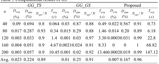
Table 5 shows the detailed results for the proposed greedy search algorithm.
(%)
avg
D is the average percentage deviation from the lower bound of the solution obtained by the algorithm described in Jackson (1956) and Dmax(%) is the maximal percentage deviation from the lower bound of the solution. Nopt is the number of problem instances (out of N, N is set to 100 in this paper) for which the solution value obtained by the corresponding algorithm equals to the lower bound. Apparently, these solutions are optimal. Tavg(s) is the average CPU time in second and Tmax(s) is the maximum CPU time in second. GG_TS is the algorithm proposed in Liaw (2008).
In order to show how much DC and GS contribute with respect to solution quality, the results obtained by GG_GS are compared to the other two algorithms.
As shown in Table 5, the proposed algorithm can find 96% optimal solutions on average, while GG_TS and GG_GS can find 89% and 91% optimal solutions on average, respectively. D s of the proposed algorithm are better than these of GG_TSavg
and GG_GS on all instance groups. Dmaxs of the proposed algorithm are better than
these of GG_TS except the instances of size 40 and size 80. Dmaxs of the proposed
algorithm are better than GG_GS on all instance groups. GG_GS requires a little more computation time than GG_TS, while the proposed algorithm requires more than 11 times of computation time than GG_TS at most.
The only difference between GG_GS and GG_TS is that they adopt different searching methods for the sequencing problem. Based on the comparison of these two algorithms, GS outperforms TS with respect to solution quality. The proposed algorithm uses DC and GG as its timetabling method which is more complicated than that of GG_GS. Because the complexity of DC is O(n2.58), calculating a timetable
consumes more CPU time with the increase of the problem size n. Therefore, the CPU time required by the proposed algorithm increases greatly with the increase of the problem size. However, it is affordable with respect to its effectiveness.
7. Conclusions
In this paper, a greedy search algorithm integrated with a divide-and-conquer-based timetabling method is proposed for the two-machine no-wait job shop problem with makespan minimization. The generic framework of the existing algorithms for the considered problem has been adopted by decomposing a problem into the timetabling problem and the sequencing problem, which were solved by the proposed divide-and-conquer-based timetabling method and a greedy search, respectively. The
proposed divide-and-conquer method (DC) can solve the timetabling problem in
) (n2.58
O complexity for a given processing sequence. Based on the results obtained by DC, a timetable enhancing algorithm converted the timetabling problem to the two-machine flow shop problem which can be optimally solved by the well-known Gilmore and Gomory algorithm (GG). A simple greedy search (GS) embedded with
DC and GG is proposed for the sequencing problem. Due to the complexity of the
timetabling method, calculating a timetable consumes more CPU time with the increase of the problem size n. Therefore, the CPU time required by GS increases greatly with the increase of the problem size. Experimental results showed that the proposed GS can find 96% optimal solutions on average. With respect to the effectiveness of the proposed GS, it is affordable.
Acknowledgements
This work is supported in part by the National Natural Science Foundation of China under Grants 60973073 and 61070160, Program for New Century Excellent Talents in University (NCET-09-0290), Qing Lan Project, and the Scientific Research Foundation of Graduate School of Southeast University (No. YBJJ0931).
References
Amir M, Zandieh M, Yazdani M, Bagheri A, 2010. A variable neighbourhood search algorithm for the flexible job-shop scheduling problem. International Journal of Production Research 48(19), 5671-5689.
Bansal N, Mahdian M, Sviridenko M (2005) Minimizing Makespan in No-Wait Job Shops. Mathematics of Operations Research 30 (4): 817–831.
Blazewicz J, Domschke W, Pesch E (1996) The job-shop-scheduling-problem: conventional and new solution techniques. European Journal of Operational Research 93: 1–33.
Dinh-Nguyen P, Andreas K (2008) Surgical case scheduling as a generalized job shop scheduling problem. European Journal of Operational Research 185: 1011–1025. Framinan JM, Schuster C (2006) An enhanced timetabling procedure for the no-wait
job shop problem: a complete local search approach. Computers & Operations Research 331: 1200–13.
Gilmore PC, Gomory RE (1964) Sequencing a one state-variable machine: a solvable case of the traveling salesman problem. Operations Research 12: 655-679.
Grabowski J, Pempera J (2000) Sequencing of jobs in some production system. European Journal of Operational Research 125: 535–550.
Graham RL, Lawler EL, Lenstra JK, Rinnooy Kan AHG (1979) Optimization and approximation in deterministic sequencing and scheduling: a survey. Annals of Discrete Mathematics 5:287-326.
Hall NG, Sriskandarajah C (1996) A survey of machine scheduling problems with blocking and no-wait in process. Operations Research 44: 510–525.
Jackson JR (1956) An extension of Johnson’s results on job lot scheduling. Naval Research Logistics Quarterly 3:201-203.
Jain A, Meeran S (1990) Deterministic job-shop-scheduling: past, present and future. European Journal of Operational Research 113 (2): 390–434.
Lenstra JK, Rinnooy Kan AHG (1979) Computational complexity of discrete optimization problems. Annals of Discrete Mathematics 4: 121–140.
Liaw CF (2008) An efficient simple metaheuristic for minimizing the makespan in two-machine no-wait job shops. Computers & Operations Research 35: 3276-3283.
Macchiaroli R, Mole S, Riemma S (1999) Modelling and optimization of industrial manufacturing processes subject to no-wait constraints. International Journal of Production Research 37(11): 2585–2607.
Mascis A, Pacciarelli D (2002) Job shop scheduling with blocking and no-wait constraints. European Journal of Operational Research 142(3): 498–517.
Meloni C, Pacciarelli D, Pranzo M (2004) A rollout metaheuristic for job shop scheduling problems. Annals of Operations Research 131: 215–235.
Ovacik I, Uzsoy R (1997) Decomposition method for complex factory scheduling problems. Dordrecht: Kluwer Academic Publishing.
Raaymakers W, Hoogeveen J (2000) Scheduling multipurpose batch process industries with no-wait restrictions by simulated annealing. European Journal of Operational Research 126: 131–151.
Rajendran C (1994) A no-wait flowshop scheduling heuristic to minimize makespan. Journal of the Operational Research Society 45(4): 472–478.
Rajkumar M., Asokan P., Vamsikrishna V., 2010. A GRASP algorithm for flexible job-shop scheduling with maintenance constraints. International Journal of Production Research 48(22), 6821-6836.
Reddi S, Ramamoorthy C (1973) A scheduling-problem. Operational Research Quarterly 24: 441–446.
Sahni S, Cho Y (1979) Complexity of scheduling shops with no-wait in process. Mathematics of Operations Research 4: 448–457.
Schuster C, Framinan JM (2003) Approximate procedures for no-wait job shop scheduling. Operations Research Letters 31:308–318.
Schuster C (2006) No-wait job shop scheduling: Tabu search and complexity of subproblems. Mathematical Methods of Operations Research 63: 473-491.
Tapan PB, Jatinder NDG, Chelliah S (2006) A review of TSP based approaches for flowshop scheduling. European Journal of Operational Research 169: 816-854. Wismer DA (1972) Solution of the flowshop scheduling-problem with no
intermediate queues. Operations Research; 20: 689–697.
Woeginger G.J., 2004. Inapproximability results for no-wait job shop scheduling. Operations Research Letters 32: 320-325.
Zandieh M, Adibi MA., 2010. Dynamic job shop scheduling using variable neighbourhood search. International Journal of Production Research 48(8), 2449-2458.
Zhu J, Li XP, Wang Q (2009) Complete local search with limited memory algorithm for no-wait job shops to minimize makespan. European Journal of Operational Research 198(2):378-386.
Table 1. Notations for two-machine no-wait job shop problems
N n : Number of jobs } , , , {J1 J2 Jn J : Set of jobs } , {M1 M2 M : Set of machines 2 , 1 , ] [ k ok i : The k th operation of [i] 2 , 1 , ] [ k pk i : The duration of ok[i] N t[i] : Starting time of [i] 2 ] [ 1 ] [ ] [i p i p i l : Duration of [i] ) , , (t [1] t [n] T : Timetable of 2 , 1 , ] [ N k tk i : Starting time of [i] on Mk
Table 2. A 10-jobs 2-machines instance
i 1 i p 2 i p s(i) 0 11 13 Ture 1 21 33 False 2 35 8 False 3 20 21 False 4 37 31 Ture 5 14 2 Ture 6 15 45 Ture 7 10 12 Ture 8 44 13 Ture 9 4 38 False
Table 3. Solutions for the instance
No. Result sequence Makespan 1 (4, 2, 8, 0, 5, 9, 3, 7, 1, 6) 248 2 (0, 6, 4, 8, 3, 9, 1, 7, 2, 5) 246 3 (4, 9, 0, 3, 7, 1, 2, 6, 8, 5) 238 4 (7, 1, 8, 0, 2, 9, 6, 3, 4, 5) 237 5 (3, 6, 9, 8, 0, 2, 5, 7, 1, 4) 236 6 (7, 6, 8, 9, 4, 1, 0, 3, 2, 5) 235 7 (6, 9, 7, 3, 4, 0, 1, 8, 5, 2) 232 8 (6, 9, 0, 5, 2, 4, 1, 8, 7, 3) 231
Table 4The time consuming of the divide and conquer timetabling method
n Tavg(ms) DC DC_GG 40 0.47 1.25 80 1.26 3.43 120 3.72 6.08 160 6.25 9.67
200 7.97 13.11 Table 5 Computational results of GS
n GG_TS GG_GS Proposed avg D (%) max D (%) Nopt/N avg T ) (s avg D (%) max D (%) Nopt/N avg T ) (s avg D (%) max D (%) Nopt/N avg T ) (s 40 0.09 0.694 0.8 0.064 0.03 0.87 0.88 0.49 0.022 0.567 0.91 0.73 80 0.017 0.287 0.93 0.34 0.015 0.29 0.88 1.46 0.014 0.20 0.89 6.18 120 0.003 0.033 0.9 1.4 0.001 0.03 0.97 3.30 0.00030.031 0.99 22.8 160 0.004 0.051 0.9 4.67 0.00210.024 0.91 8.33 0 0 1 68.82 200 0.003 0.057 0.9 10.45 0.001 0.02 0.92 13.460.00020.019 0.99 147.12 Avg. 0.023 0.224 0.89 0.01 0.25 0.91 0.007 0.167 0.96 2 ] [i p 1 ] [i p 1 ] [i p 2 ] [i p 2 ] [i o 1 ] [i o 1 ] [i o 2 ] [i o Positive Negative
Fig. 1 A positive job and a negative job
2 ] [i t (a) (b) (c) (d) (e) (f) 2 ] 1 [i t 2 ] [i t 2 ] 1 [i t 2 ] [i t 2 ] 1 [i t 2 ] [i t 2 ] 1 [i t 2 ] [i t 2 ] 1 [i t 2 ] [i t 2 ] 1 [i t
Fig. 2 Gantt charts of the feasible timetable for possible two jobs
] [k ] [k [k] ) , ([k][n] ) , ([1][k]
overlapFig. 3. Profile of Gantt chart for two subsequences when [k][k] ) , ([k][n] ] [k ] 1 [k [k1] [k]
] [k ] 1 [k
overlap ) , ( [1] [k]Fig. 4. Profile of Gantt chart for two subsequences when [k][k1]
/*Base case (1)*/ Function OPT_B1(,)
1. sum 0, overlap 0
/*Calculating the sum of all super jobs*/ 2. For i 1 to | |
/*If [i] [i1], the super job has been visited*/
If [i] [i1], ) , ( [] [] max sum C i i sum
/*Calculating the sum of overlaps
between any two consecutive super jobs*/ 3. For i1 to | |1 3.1 If [i] [i1],i i1 3.2 j i1 3.3 If [j] [i], j j1 3.4 ) , , , ( [] [] [ ] [ ] overlap Overlap i i j j overlap
4. Return sumoverlap
/*Calculating the duration of a super job*/ Function Cmax([i],[i] )
Return max{ , } max{ , 2 }
] [ 2 ] [ 1 ] [ 1 ] [i p i p i p i p
/*Calculating the maximal overlap of two super jobs*/ Function Overlap([i],[i],[j],[j]) 1. max{ , } max{ , 1 } ] [ 1 ] [ 2 ] [ 2 ] [i p i p j p j p ; 2.1 max{([i])12,([i])12}max{([j])11,([j])11} 3.2 max{([i])22,([i])22}max{([j])21,([j])21} 4. max{1,2} 5. Return
Fig. 5. The pseudocode for Base case (1) overlap } , max{p2[i] p2[i] } , max{p1[i] p1[i] [i],[i] [j],[j]
Fig. 6. Maximal overlap of two consecutive super jobs /*Base case (2)*/
Function OPT_B2(,,l) 1. [l] [l]
/*At this point, all jobs’ partners in the current sequence are determined*/
2. cmax OPT_B1(,) 2. Return cmax
Fig.7. The pseudocode for Base case (2) /*Base case (3)*/ Function OPT_B3(,,l,f) 1. cmax 0 2. If s([l])s([f]) 2.1 [l] [l],[f] [f] 2.2 cmax OPT_B1(,) 3. If s([l])s([f]) 3.1 [l] [f],[f] [l], c1 OPT_B1(,) 3.2 [l] [l],[f] [f], c2 OPT_B1(,) 3.3 cmax min{c1,c2} 4. Return cmax
Fig.8. The pseudocode for Base case (3)
Function OPT(,)
1 If [i] NULL(i1, |, |),l 1, f 1;
Elselmax{i|[i] NULL,i1, |, |}, f min{i|[i] NULL,i 1,|, |}; /*Step 2~4 deal with the base cases*/
2. If l f 1, return OPT_B1(,); 3. If l f 0, return OPT_B2(,,l); 4. If l f 1, return OPT_B3(,,l,f); /*k is the index of the key job for the division*/ 5. 2 f l k /* DC_Case (1) */ 6. If s([k1])s([k])s([k1]),[k] [k], cmax )) , ( ), , ( ( )) , 1 ( ), , 1 ( ( k k OPT k n k n OPT }) , max{ } , (max{ 2 ] [ 2 ] [ 1 ] [ 1 ] [k p k p k p k p /* DC_Case (2) */ 7. Ifs([k1])s([k])and s([k])s([k1]) 7.1 [k] [k]; 1 c OPT((1,k),(1,k))OPT((k,n),(k,n)) }) , max{ } , (max{ 2 ] [ 2 ] [ 1 ] [ 1 ] [k p k p k p k p ; 7.2 [k] [k1], [k1] [k]; )) , ( ), , ( ( )) 1 , 1 ( ), 1 , 1 ( ( 2 OPT k k OPT k n k n c } , max{ } , (max{ 2 ] 1 [ 2 ] 1 [ 1 ] 1 [ 1 ] 1 [ p k p k p k p k ; 7.3 cmax min{c1,c2}; 7.4 If cmax , c1 [k] [k]; else [k] [k1], [k1] [k]; /* DC_Case (3) */ 8. If s([i1])s([i]), s([i])s([i1]) 8.1 [k] [k]; 1 c OPT((1,k),(1,k))OPT((k,n),(k,n)) }) , max{ } , (max{ 2 ] [ 2 ] [ 1 ] [ 1 ] [k p k p k p k p ;
8.2 [k] [k1], [k1] [k]; 2 c OPT((1,k),(1,k))OPT((k1,n),(k1,n)) }) , max{ } , (max{ 2 ] [ 2 ] [ 1 ] [ 1 ] [k p k p k p k p ; 8.3 cmax min{c1,c2}; 8.4 If cmax c1, [k][k]; else [k][k1], [k1][k]; /* DC_Case (4) */ 9. If s([i1])s([i1]),s([i])s([i1]) 9.1 [k] [k]; 1 c OPT((1,k),(1,k))OPT((k,n),(k,n)) }) , max{ } , (max{ 2 ] [ 2 ] [ 1 ] [ 1 ] [k p k p k p k p ; 9.2 [k] [k1], [k1] [k]; 2 c OPT((1,k),(1,k)) OPT((k1,n),(k1,n)) }) , max{ } , (max{ 2 ] [ 2 ] [ 1 ] [ 1 ] [k p k p k p k p ; 9.3 [k][k1], [k1] [k]; 3 c c3OPT((1,k1),(1,k1)) OPT((k,n),(k,n)) }) , max{ } , (max{ 2 ] 1 [ 2 ] 1 [ 1 ] 1 [ 1 ] 1 [ p k p k p k pk ; 9.4 cmax min{c1,c2,c3} 9.5 If cmax , c1 [k] [k]; Else if cmax c2[k] [k1], [k1] [k]; Else [k] [k1], [k1] [k]; 10. Return cmax
Procedure Divide_and_Conquer()
1. (NULL , ,NULL),cmax 0, n| |
) 1 , , 1 , 0 ( ) , , (t [1] t [n] T 2. cmax OPT(,) 3. For i2 to n 3.1 If [i] [i], t[i]max{t[i1]l[i1],t[i1] l[i1]}
) , , , ( [ 1] [ 1] [] [] ] [ ] [i t i Overlap i i i i t 3.2 If [i] [i1],t[i] max{t[i1] l[i1],t[i1] l[i1]} ) , , , ( [ 1] [ 1] [] [] ] [ ] [i t i Overlap i i i i t } , max{ 1 ] 1 [ 1 ] [ ] [ ] [i t i p i p i t 1 ] 1 [ ] [ ] 1 [i t i p i t 1 ] [ ] [ ] [i t i p i t
/*T(t[1],,t[n]) is the optimal timetable with the minimal cmax*/ 4. Stop
Fig. 9. The pseudo-code of DC timetabling method
![Table 1. Notations for two-machine no-wait job shop problems Nn : Number of jobs },,,{J 1 J 2 J nJ : Set of jobs },{M 1 M 2M : Set of machines 2,1 ] ,[ k oki : The k th operation of [i ] 2,1 ] ,[ k p k i : The duration of o k [ i ] Nt [ i](https://thumb-eu.123doks.com/thumbv2/123doknet/14131543.469135/19.892.124.462.748.971/table-notations-machine-problems-number-machines-operation-duration.webp)
![Fig. 4. Profile of Gantt chart for two subsequences when [ k ] [ k 1 ]](https://thumb-eu.123doks.com/thumbv2/123doknet/14131543.469135/21.892.228.666.418.1159/fig-profile-gantt-chart-subsequences-k-k.webp)
![Fig. 5. The pseudocode for Base case (1) overlap },max{p 2 [ i ] p 2 [ i ] },max{p1[i]p1[i] [i],[i] [ j ] , [ j ] ](https://thumb-eu.123doks.com/thumbv2/123doknet/14131543.469135/22.892.204.686.107.1039/fig-pseudocode-base-case-overlap-max-p-max.webp)

