Authentication protocol using trapdoored matrices

Authentication Protocol using Trapdoored Matrices

by

Aikaterini Sotiraki

Submitted to the Department of Electrical Engineering and Computer

Science

in partial fulfillment of the requirements for the degree of

Master of Science

at the

MASSACHUSETTS INSTITUTE OF TECHNOLOGY

February 2016

@

Massachusetts Institute of Technology 2016. All rights reserved.

Author ..

Signature redacted

Depariii7iift

Electrical Engineering and Computer Science

November 16, 2015

Certified by...Signature

redacted

Ronald L. Rivest

Professor

Thesis Supervisor

Accepted by ...

Signature redacted

L'eslieCWN kolodziej ski

Graduate Officer, Department Committee on Graduate Theses

MASSACE SN TITUTE

Authentication Protocol using Trapdoored Matrices

by

Aikaterini Sotiraki

Submitted to the Department of Electrical Engineering and Computer Science on November 16, 2015, in partial fulfillment of the

requirements for the degree of Master of Science

Abstract

In this thesis, we propose a new type of public-key authentication protocol, which is based on timing gaps. The honest user's secret key allows him to perform a task faster than any adversary. In our construction, the public key is a n x n matrix and the secret key is a trapdoor of this matrix. The task which an honest user has to perform in order to authenticate himself is a matrix-vector multiplication, where the vector is supplied by the verifier. We provide specific constructions of the trapdoor and analyze them both theoretically and practically.

Thesis Supervisor: Ronald L. Rivest Title: Professor

Acknowledgments

This work was supported by Paris Kanellakis Fellowship and Akamai Fellowship. I would like to express my gratitude to my supervisor, Ron Rivest, for the useful discussions and engagement through the learning process of this master thesis. Also, I would like to thank Yuval Peres for the very helpful feedback on the theory of Markov chains.

Contents

1 Authentication protocols

1.1 Introduction . . . .

1.1.1 Authentication Protocols . . . . 1.2 Time-based authentication protocols . . . . 1.2.1 General form of the protocol . . . . 1.2.2 Protocol based on computing a 2 (mod n)

1.2.3 Protocol based on Trapdoored Matrices .

2 Theoretical background

2.1 Linear Algebra . . . .

2.2 Markov Chains . . . . 2.2.1 Basic Definitions and Theorems . . . . 2.2.2 Strong Stationary Time . . . . 2.3 Matrix-vector multiplication . . . .

3 Protocol Analysis

3.1 Adversarial model . . . .

3.2 Candidate trapdoor construction . . . . 3.3 Protocol Security . . . .

3.3.1 Markov Chain and Stationary distribution . . . . 3.3.2 One-column case . . . .

3.3.3 One-row case . . . . 3.3.4 Expected number of elements equal to x E GF(q)

9 . . . . 9 . . . . 9 . . . . 13 . . . . 14 . . . . 14 . . . . 16 19 . . . . 19 . . . . 21 . . . . 22 . . . . 25 . . . . 26 29 29 . . . 30 31 31 . . . 33 38 40

3.4 Other Trapdoor Constructions . . . . 42

4 Implementation in practice 45

4.1 Characteristics of smart cards . . . . 45 4.2 Suggestions on the protocol parameters . . . . 46

Chapter 1

Authentication protocols

1.1

Introduction

Authentication is a problem that arises in various settings and there are many different proposals for solving it. In this thesis, we consider authentication in the public-key setting. We start by explaining what authentication is and describing some previous protocols for achieving it. Afterwards, we provide our suggestion. In the following chapters, we present the necessary background for analyzing our protocol. We give a more concrete description of the protocol and we conclude with some considerations on its implementability.

In this chapter, we define what authentication is. We outline our proposal and describe some previous work on authentication.

1.1.1

Authentication Protocols

An interactive public-key authentication protocol is a protocol in which there are two parties, a prover and a verifier. The prover wants to authenticate herself to the verifier by proving the possession of the secret key connected to her public key. During the setup phase of the protocol, the verifier acquires some information that he trusts regarding the prover. For instance, a trusted authority might tie together the public key and the name of the prover in a certificate, which the verifier can then

access, or the prover might add his public key to a public directory. If the execution of the protocol is successful, then the verifier knows that the information the prover provides is consistent with the trusted information.

Usually an authentication protocol consists of two stages. In the first one, the verifier poses a challenge to the prover. In the second one, the prover proves that she knows the secret key by answering the challenge correctly. The development of zero-knowledge proofs in this setting is very useful. The prover wants to authenticate herself, but at the same time she needs to make sure that the verifier, or any eaves-dropper, learns nothing about her secret key, apart from the fact that she knows it. This is exactly what a zero-knowledge proof of knowledge offers [9].

The notion of authentication we use is the following [81:

Definition 1. A scheme is an authentication scheme if A can prove to B that she is

A, but someone else cannot prove to B that she is A.

The definition of a secure authentication system scheme is, then, similar to that of a secure identification system scheme of Feige et al. [71:

Definition 2. An authentication system scheme is secure if for any polynomial

en-semble of users the probability of an impersonation event in a randomly chosen au-thentication system is negligible. In this case, an impersonation event is the event that at least once during the lifetime of the system one user succeeds in authenticating himself as some other good user, namely a user that throughout the lifetime of the system does not deviate from the protocol dictated by the scheme.

Some examples of authentication protocols are a protocol by Fiat and Shamir [8] and a protocol by Schnorr

[201.

Both of these protocols base their security on some number theoretic problems which are believed to be intractable. The prover's secret key is a quantity that no dishonest party can compute because of the intractability assumption. As usual, the authentication protocol is based on answering the challenge posed by the verifier correctly in zero-knowledge. The protocol is secure if no dishonest party can answer correctly the challenge in polynomial time.

Fiat-Shamir protocol

At CRYPTO'86 conference, Fiat and Shamir presented an authentication protocol based on the difficulty of factoring [81. In their protocol, they assume the existence of a trusted center. This center publishes the universal parameters:

1. a large composite number n, which is the product of two primes, p and q,

2. a pseudo-random function,

f,

which maps arbitrary strings to the range [0, n),

3. two small integers k and t.

The center, also, issues the private keys of the users with the following procedure:

" Create a string I with all the information about the user and the card.

" Compute the values vj = f(Ij) for small values of

j.

" Pick k distinct values of

j

such that Vj is a quadratic residue modulo n.

" For each

j

that was picked, compute the smallest square root sj of t.), i.e. the smallest sj such that sj .'v = 1 (mod n).

" Issue a smart card which contains I and the k values sj with their indices.

Then, the authentication protocol is the following, where we assume that the k values of j used are {1, ... , k1:

1. The prover sends I to the verifier.

2. The verifier computes vj = f(I, j) for

j E

{1, ... , k}.

3. Repeat the following steps for i 1 t:

(a) The prover picks a random ri E [0, n) and sends xi = ri (mod in) to the verifier.

(b) The verifier sends a vector (el, ... , eik) E {0, 1}k to the prover.

(d) The verifier checks if xi = y'

H~

vj (mod n).

e'i=1

4. If the t checks are successful, the verifier accepts. Otherwise, he rejects.

Schnorr protocol

At CRYPTO'89 conference, Schnorr presented another authentication protocol based on the difficulty of computing the discrete logarithm [201. In this protocol, the uni-versal parameters published by the trusted center are the following:

1. two large primes, p and q such that qI(p - 1), 2. an a E Zp with order q,

3. a small integer t.

The center has its own public/private key pair for signing the users' public keys. It registers a user by creating a string I with all the information about the user and the card and signing (I, v), where v is the user's public key.

Each user generates his private key s and his public key v by himself: * The private key s is a random number in {1, 2,.q}.

* The public key v is the number v = a~" (mod p). Then, the authentication protocol is the following:

1. The prover sends I, t) and the trusted center's signature of (I, v) to the verifier.

2. The verifier verifies the center's signature transmitted by the prover.

3. The prover picks a random r E {1.q - 1} and sends x = ar (mod p) to the verifier.

4. The verifier sends a random number e

c

{0,..., 2t - 1} to the prover. 5. The prover sends y = r + s - e (mod p) to the verifier.

6. The verifier checks if x = dC - " (mod p).

1.2

Time-based authentication protocols

In this work, we present an alternative idea for creating authentication protocols. The major component in our protocol is not the response to a challenge, but the time needed to provide this response. The verifier keeps track of the time that the prover needs in order to respond correctly. Only if this time is small enough and the answer is correct does the prover authenticates herself successfully. More precisely, the secret key is a trapdoor that gives the honest party a polynomial time advantage in answering the challenge.

Time plays an important role in many cryptographic protocols, especially as far as their security is concerned. Many protocols, such as Diffie-Hellman, RSA and DSS, can be broken using timing attacks [111. In these cases, measuring the difference between the time needed to perform different computations gives the adversary a non-negligible advantage and breaks the security of the protocol. Other identification protocols (e.g. [51) use the timing delay between the challenge and the response as a "distance bounding" technique. This technique is then integrated in an identification protocol, so that the verifier can verify not only the identity of the prover, but also that she is close by. A case in which this is helpful is the identification at the entrance to a building, where the prover has to show that she is present there.

In contrast to other authentication protocols, in our protocol, the dishonest party is able to find the correct answer to the challenge, but to do so he needs an unac-ceptable amount of time. A polynomial gap between the time of the honest party and the best time of the adversary is enough to make our protocol work. This notion of polynomial gap is not new in cryptography. For example, Merkle's puzzles [131, an early proposal related to public-key cryptography, were based in the quadratic difference in the complexity for the honest and the dishonest party.

Informally, an authentication protocol based on timing gaps is secure if, given the public key of a user, no polynomial adversary can find a way to accelerate its computation enough to fool the verifier. To facilitate the description and construction of such protocol, we need to make some assumptions. As mentioned before, a very

important assumption is that the verifier has obtained the prover's correct public key. Then, he checks that the prover can authenticate herself in a way consistent with the trusted information. Furthermore, we assume that the person authenticating herself with a time-based protocol has an implementation whose running time is independent of the starting time of the protocol execution. This means that we can consider that the time the prover needs to answer the challenge is constant over time. Similarly, we assume that the time needed to complete the protocol is independent of the trapdoor and the challenge. So, no timing attacks can be applied to our protocol.

Our proposal suggests that even a polynomial gap between the time needed to successfully complete a challenge with and without the secret key is enough to con-struct an authentication protocol. Such a protocol could be used in authentication via smart cards. For instance, the verifier could be an ATM and the prover could be the smart card that a customer uses.

1.2.1

General form of the protocol

The general form of a scheme based of a polynomial timing gap is shown in Figure

1-1. In our case, we are not interested in problems that are solvable to someone that

possesses certain information, but are intractable without this information. We are interested in problems that can be solved by anyone, but faster with certain trapdoor information than without it.

1.2.2

Protocol based on computing

a2t

(mod

n)

We demonstrate how a time-based authentication protocol works with a protocol that is based on the ideas about time-lock puzzles [19]. A time-lock puzzle is a puzzle which no one, except maybe its creator, can solve without running an algorithm for at least a certain amount of time. In our case, the creator of the puzzle is the prover; this gives her the ability to find the solutions faster than anyone else.

The protocol is the following:

VERIFIER

Figure 1-1: Time-based authentication protocol. key. The prime numbers p and q are the secret key.

o Whenever the prover wants to authenticate herself to the verifier, she asks for a number t E N.

o The verifier generates a random, but of appropriate size, t E N and a random a E Z* and sends them to the prover.

o The prover computes quickly, using the factorization of n, the quantity c = 2t (mod 0(n)) then she sends back to the verifier y = ac (mod n).

o The verifier verifies that y = a2t (mod n) by performing the usual exponentia-tion, using the publicly available modulo n.

Starts timer

Sends a challenge

Computes answer

using her secret key

Sends the answer

Stops timer

Checks if the time

needed is small

"enough" and the

answer is correct.

If yes, he accepts.

Otherwise, he rejects

* If y is correct and the time the prover needed is "sufficiently small", then the verifier accepts. Otherwise he rejects.

Without knowing the factorization of n, the fastest way to compute a2 (mod n) seems to be to start with a and perform t squarings sequentially. So, the fact that the prover knows the factors p and q gives her an advantage in the time needed to find the desired result.

In the above protocol, we mention that the number t that the verifier chooses should be of appropriate size. If t is too small, then the time needed by the prover does not differ a lot by the time an adversary needs, which might make it difficult for the verifier to distinguish honest from dishonest parties. On the other hand, if t is too large, then the time needed by the verifier in order to compute a2t (mod n) might be too much, which again is a problem since the verifier cannot accept or reject before computing this quantity by himself.

1.2.3

Protocol based on Trapdoored Matrices

Another suggestion for implementing time-based authentication is through trapdoored matrices. This is the type of protocol we are concerned in the next chapters.

In this protocol, a user's public key consists of an n x n matrix A over GF(q), where q is fixed, and her secret key is a trapdoor of A. The challenge is to perform the computation Ax for a random n-vector x as fast as possible. The protocol is of the following form:

" The prover creates a trapdoored n x 77 matrix A over GF(q) and publishes it

as her public key.

" Whenever the prover wants to authenticate herself to the verifier, she asks for

a 'n-vector x with elements over GF(q).

" The verifier generates a random vector x E GF(q)"' and sends it to the prover.

" The prover computes very quickly, using the trapdoor, the quantity y = Ax and sends it back to the verifier.

o The verifier verifies whether y = Ax in 0(n2

) time with the naive matrix-vector multiplication using the public matrix A.

o If y is correct and the time the prover needed is "sufficiently small", then the verifier accepts. Otherwise, he rejects.

We denote the trapdoor of matrix A by T(A). This trapdoor must give a signifi-cant advantage to the prover in terms of the time she needs in order to perform the operation Ax. For instance, the trapdoor could be a compact straight-line program for computing Ax. Simultaneously, it should be difficult for an adversary to find a trapdoor, which would allow him to perform this operation quickly enough to trick the verifier.

In the next chapters, we describe a candidate construction of the trapdoored matrix A.

Chapter 2

Theoretical background

In the chapter, we give some necessary background for analyzing the construction of trapdoored matrices. For this construction .we need some basic notions of linear algebra and of Markov chains. We start this chapter with some definitions and facts of linear algebra. We continue with an overview of Markov chains, focusing especially on methods we will use afterwards.

In the next chapter, we present some analysis of the asymptotic complexity of matrix-vector multiplication over GF(q) using the trapdoor. We want this complexity to be smaller than the best known algorithm for matrix-vector multiplication. So, we conclude this chapter with a brief presentation of the previous works on measuring the complexity of matrix-vector multiplication.

2.1

Linear Algebra

In the proposed protocol, we pick our trapdoored matrix to be full rank. Even though we do not really need invertibility, the complexity of the matrix-vector multiplication for full rank matrices is at least as large as that for those with lower rank. Since we aim at distinguishing honest from dishonest parties based on small time differences in computing a matrix-vector multiplication, we want to minimize the time needed

by the honest user. This is done by using the best possible trapdoor. Simultaneously,

restrict our attention to full rank matrices.

We denote the i-th row of an n x TI matrix A by A. Then, from elementary linear

algebra:

Definition 3. An elementary row operation on a matrix A is one of the following:

1. Row switching: Switch row i and row

j

of the matrix (.4 -+ Aj)

2. Row multiplication: Replace row i by its multiplication with a non-zero k (A

<-k - 4j

3. Row addition: Substitute row i by its sum with a multiple of row

j

(A

+-Ai + k - Aj)

Definition 4. An elementary matrix is a matrix that is produced by performing a

single elementary row operation on the identity matrix.

Theorem 5. An n x n matrix is invertible if and only if it can be written as a product

of elementary matrices.

The representation of an invertible matrix as a product of elementary matrices is closely related to Gaussian elimination. Each step of Gaussian elimination is a single elementary row operation, so it can be represented as a multiplication with an elementary matrix. This means that every invertible matrix can be written as a product of at most O(n2_{) elementary matrices.}

For our purpose we use a slightly different notion of elementary row operation:

Definition 6. A general row operation on a matrix A is the substitution of row Ai

by a - Ai + b - Aj where j is another row and a

c

GF(q) \ {}, b

E

GF(q).

Similarly to the above, we define the notion of a general elementary matrix. Each general row operation can be expressed as a sequence of at most 2 elementary row operations, a row multiplication (if a

$

1) and a row addition (if b = 0). Also: Lemma 7. Every elementary row operation on a matrix A can be expressed as

Proof. * Row switching: 1. Aj<-1-Ai--A 2. Aj <- - A + - Ai 3. Ai+--1- Ai+1-A * Row multiplication: Ai +- k - Ai + 0 -A

*

Row addition:

A

*- 1 - Ai + k -Aj

So, from Theorem 5 and Lemma 7 we have that

Proposition 8. A matrix can be written as a product of 0(n2) general elementary matrices if and only if it is invertible.

Theorem 8 is the basic tool we use for creating the trapdoor. Each trapdoored matrix is the product of L(n) general elementary matrices. The prover knows these matrices and their order in the multiplication, while the verifier only knows the re-sulting product.

In next chapters, we also use the following proposition:

Proposition 9. A general elementary matrix is invertible and its inverse is also a

general elementary matrix.

Proof. If A is a general elementary matrix corresponding to the row operation Ai

+-a - Ai

+

b - Aj with a z 0, then the general elementary matrix corresponding to the

row operation Ai +- a-1 -A - a-1 - b - Aj is its inverse.

2.2

Markov Chains

As we mentioned in the previous section, each public key is the product of general elementary matrices. We denote the number of elementary matrices on the product, which also determines the size of the trapdoor, by L(n). We know that each invertible

matrix can be written as a product of general elementary matrices (Proposition 8).

So, in order to analyze the security of the protocol, we need to find the size of

L(n) for which it is hard to distinguish a trapdoored matrix produced as a product of L(n) random general elementary matrices from a completely random invertible matrix. This question is strongly related to the theory of Markov chains. This section mentions the basic definitions and methods we need ( [14], [2], [12]).

2.2.1

Basic Definitions and Theorems

We start by defining what a Markov chain is:

Definition 10. A sequence of random variables X₀, X1, N2, ... is a Markov chain with state space Q if for all a0, a1,..., at E Q it satisfies the Markov property:

Pr(Xt = atIXt-1 = at-_, Xt_2= at-2, , XO= ao) Pr(Xt = atIXt_1 = at-)

If Q is finite, then the Markov chain is called finite Markov chain.

For the rest of the section, we consider only finite Markov chains.

Definition 11. The transition probability

Pi,; = Pr{ Xt = |Xt_ I)

is the probability that the process moves from state i to j in one step.

The Markov property implies that the Markov chain is uniquely defined by the one-step transition matrix:

P₁,1 P1,2 P, ... P1,n

Pi,1 Pi,2 Pij - -

n

Pnn-This matrix is called the transition matrix of the Markov chain.

Definition 12. A Markov chain is irreducible if all states belong to one

communi-cating class. Namely, for any two states i, j E Q there exists an integer t such that

Pt(ij)

>

0.

Definition 13. A state i in a discrete time Markov chain is periodic if there exists

an integer K > 1 such that P(Xt+ = iIXt = i) = 0 unless s is divisible by K. A discrete time Markov chain is periodic if any state in the chain is periodic. A state or a chain that is not periodic is aperiodic.

A very useful notion in Markov chains is that of the stationary distribution, which

shows the limiting distribution over the state space of the chain. We are interested in finding the stationary distribution of specific chains and arguing that there is only one stationary distribution. So, the following propositions are helpful.

Definition 14. A stationary distribution (also called an equilibrium distribution) 7

of a Markov chain is a probability distribution 7r such that:

7 = r - P

Definition 15. A matrix is called doubly stochastic if its row sums and its column

sums are 1.

Theorem 16. The stationary distribution of a Markov chain with doubly stochastic

transition matrix is the uniform distribution over Q.

Definition 17. A state i is called absorbing if the chain never leaves i once it first

visits i. Namely, Pjj = 1 and, of course, Pj = 0, for all j f i.

If every state can reach an absorbing state in a finite number of steps, then the chain is called absorbing Markov chain.

Proposition 18. ( [12] Proposition 1.26) If an absorbing Markov chain has a unique

absorbing state i, then it has as unique stationary distribution the degenerate distri-bution at i.

Another very useful notion is that of mixing time, which shows how quickly a Markov chain approaches its stationary distribution. We formally define this notion and in the next section, we describe famous methods for bounding it.

Definition 19. The variation distance between two distributions D1 and D2 on a

countable state space Q is given by

ID

₁ - D2

11

= jD1(i) - D2(i)I

iEQ

Definition 20. Let 7r be the stationary distribution of a Markov chain with state

space Q. Let P1' represent the distribution of the state of the chain starting at state i after t steps. We define

AX(t) = ||PFl - 7r||

and

A(t) = max Ai(t).

iEQ

That is, Ai(t) is the variation distance between the stationary distribution and Pt, and A(t) is the maximum of these values over all starting states i.

We also define

T-(e) = min{t : Ai(t) < E};

and

T(E) = maxri(E). iEf

That is, Ti(E) is the first step t at which the variation distance between P19 and the stationary distribution is less than e, and T(E) is the maximum of these values over all states i.

Definition 21. When T(E) is considered as a function of E, it is called the mixing time of the Markov chain.

Theorem 22. (Convergence Theorem [12]) Suppose that P is irreducible and

ape-riodic. Then, it has a unique stationary distribution 7r. Also, there exist constants a E (0, 1) and C > 0 such that

max IPt - IrI ITV ; Cat.

2.2.2

Strong Stationary Time

One of the basic tools to analyze the mixing time of a Markov chain is the notion of strong stationary time. This section provides the basic definitions and theorems we need about the strong stationary time.

Definition 23. Given a sequence (Xt)g0 of Q-valued random variables, a {0, 1, 2,..., oo}-valued random variable T is a stopping time for (Xt) if, for each t E {0, 1,...}, there is a set Bt C Qt+1 such that

{T = t} = {(X₀, X1,..., Xt) E Bt}.

In other words, a random time T is a stopping time if and only if the indicator function 1,t is a function of the vector (Xo, X1 ... , X,).

Proposition 24. Every transition matrix P on a finite state space has a random

mapping representation: we can find a function f : Q x A -+ Q, along with a A-valued

random variable Z, satisfying

P(f (i, Z) = A) = Pij.

Therefore, if (Z,)-'f 1 is a sequence of independent random variables, each having the same distribution as Z, and X0 has distribution p, then the sequence (Xt)Co defined

by

is a Markov chain with transition matrix P with starting distribution ft.

Definition 25. A random time T is called a randomized stopping time for the Markov

chain (Xt) if it is a stopping time for the sequence (Zr).

Definition 26. A strong stationary time for a Markov chain (Xt) with stationary

distribution 7r is a randomized stopping time T, possibly depending on the starting

position i, such that

Pi (7 = t, -X, = j)] = Pi (T = t) 7r )

Theorem 27. [12] If T is a strong stationary time, then

A (t)

<;

Max Pi (T > t).

iEO

2.3

Matrix-vector multiplication

The naive algorithm for matrix-vector multiplication over finite fileds has complexity 6(n2). However, there are many algorithms that achieve better complexity. The most well-known algorithm for matrix-vector multiplication over GF(2) with complexity less than O(n 2) is known as the Four Russians' Algorithm ( [4], [1]). Its running time

it

o(-!

), but it requires auxiliary storage of 0( L)) bits.

The best known algorithm to perform matrix-vector multiplication over GF(q) [21] has running time 0( 2) for any e

C

(0, 1). An important aspect of this algorithm

is that it requires some amount of preprocessing. In our protocol, preprocessing is permitted, since the n x n matrix is the public key. The adversary can spend any polynomial amount of time in preprocessing this matrix, so that when he receives the challenge vector he can perform the operation as fast as he can. More formally, the theorem (expressed for finite fields) of Williams [211 states:

Theorem 28. Let GF(q) be a finite field of q elements. For all c E (0,1), every Pn x n

matrix A over GF(q) can be preprocessed in O(n 2

subse-quent matrix-vector multiplication can be performed in O( 21) ) steps on a pointer machine or a (log(n))-word RAM, assuming operations in GF(q) take constant time.

Apart from the known algorithms for matrix-vector multiplication, there are some known lower bounds for the problem and conjectures about what the lower bounds should be. A lower bound of Q(n2

) arithmetic operations is known [221. However, one of the assumptions of that result is that the underlying field should be infinite.

More recently Henzinger et al. [101 addresses the problem of Online Boolean Matrix-Vector multiplication. In this problem, we want to compute a n x 71 matrix multiplication A- B, but we are given one column-vector of B, vi, at each round. After seeing each vector vi, we have to output the product A - vi before receiving the next vector. The paper shows that a conjecture that there is no truly subcubic (O(n'-))

algorithm for the Online Boolean Matrix-Vector multiplication problem can be used to prove the underlying polynomial hardness appearing in many dynamic problems. It is easy to see that this problem is a generalization of the Matrix-Vector multiplication in which we are interested.

Chapter 3

Protocol Analysis

We begin this chapter with a description of the adversarial model we use. Then, we outline our candidate construction for the trapdoor matrices. In the following sections, we analyze the security of the protocol using theoretical arguments and experimental results.

3.1

Adversarial model

To argue the security of a protocol, it is necessary to first describe the adversarial model considered. In our case, we assume that the adversary has "comparable" power with the honest user. That means that the adversary is restricted to polynomial time algorithms.

As we have already mentioned, we focus on the scenario of the authentication of an honest party to an ATM using smart cards. So, we consider adversaries who know the authentication protocol and its public parameters, the honest party's public key and the type of smart card used. Then, they use all the known information to create a fake smart card and try to fool the ATM. Since our protocol is based on a very parallelizable problem (matrix-vector multiplication) and smart cards have very limited computational capabilities, we assume that the adversary can use the best available smart card, even if this is better than that of the honest user. However, he cannot connect it to external devices that can perform faster, maybe parallel,

computation.

In a later section, we try to find practical parameters for our protocol. Of course, the adversarial power affects these parameters. A concrete example is the size of the public key, which is a n x n matrix. On one hand, we need n to be as small as possible, so that the trapdoor and challenge fit in the storage of the smart card. On the other hand, the time to perform the regular matrix-vector multiplication depends on n. So, n has to be large enough, so that the adversary needs noticeably more time, say tenfold, than the honest user in order to find the result of the computation.

3.2

Candidate trapdoor construction

This section presents our construction for the trapdoored matrix A as a product of L(n) random general elementary matrices. We argue that, given such a matrix A, it is difficult to factorize it as a product of O(L(n)) general elementary matrices. Then, the best strategy for any adversary would be to perform the fastest possible matrix-vector multiplication and return the result. If the complexity of matrix-vector multiplication is f(n) and we pick L(n) = o(f(n)), then for large enough n the honest party has a noticeable timing advantage in computing the product Ax.

The procedure that a user follows to create a trapdoored matrix A is the following: For k 1, ... , L (n)

" Pick ik uniformly at random from {1.,n}

" Pick

jA

uniformly at random from {1, ... , n}

\

{ik}

" Pick ak uniformly at random from GF(q) \ {O}

" Pick bk uniformly at random from GF(q)

Then,

4

= A(L) - 4( ) - ... A()

where A(k) is the general elementary matrix corresponding to the operation A a -Aik + bk . Ajk.

Thus, the trapdoor T(A) consists of the sequence of L(n) tuples:

(ik, jk, ak, bk), for k =1, 2, ... , L

We force ik

#

JA, because we want the matrix A to be invertible.

The program that the honest party uses in order to take advantage of the knowl-edge of the trapdoor begins by copying y = x, that is y, = xi for 1 < i < n. Then, the k-th step, for 1 < k < L, has the form:

Yik = ak yik + bk .Yjk.

The final value of y = (y1, Y2, - yn) is the output. The complexity for the honest user in e(L(n)).

3.3

Protocol Security

The previous section describes how to create a trapdoored matrix using L(n) random general elementary row operations. In this section, we estimate how big L(n) should be so that the resulting matrix is indistinguishable from a random invertible matrix to any polynomial time adversary.

3.3.1

Markov Chain and Stationary distribution

The process of producing a trapdoored matrix yields a sequence of random variables with state space Q = GL(n, q), the set of all invertible n x n matrices over GF(q), which satisfies the Markov property. So, this process defines a finite Markov chain,

M.

Claim 29. The unique stationary distribution of M is the uniform on GL(n, q).

This claim is indispensable in showing the security of the protocol. If we allow L(n), the number of tuples in the trapdoor T(A), to be large enough, then we end up with an approximately uniformly random matrix in GL(n, q). So, for large enough

L(n), no adversary can tell whether a matrix was produced by the previous process or not.

We cannot hope to set L(n) equal to Tni because we know a lower bound on iu

of ('n2/ logq(n)). To see that, we create a graph with vertex set Q and edges between states A and B for which P4,B + PA,B > 0. We know that the diameter, diam, of

this graph, for fixed q, is 0(n2

/

logq(n)) [3]. Then, from the general lower bound on mixing time Tmij > ldiam [121, we get that 1s =(nQ

2

/

Proposition 30. The transition matrix of M, P, is symmetric.

Proof. We show that PA,B = PB,A, for all A,B E GL(n,q).

* If PAR,= 0, then PB,A= 0. By contradiction: If PB,A

#

0, then there is a

general elementary matrix C such that B = C - A. But then, A = C- - B and

from Proposition 9, C-' is a general elementary matrix. So, PAB

$

0, which is

a contradiction.

* If PA,B = 0, then there is a unique general elementary matrix C such that

B = C - A. Again from Proposition 9, C 1is a general elementary matrix. The

uniqueness comes from the fact that A is invertible, so C = B -A-1.

Since at each step of the Markov chain we pick a random general elementary matrix to multiple the current state and there is only one such matrix that moves state A to state B and conversely, PA,B =

PB,A-Proof. (Claim) Since P is a transition matrix, the sum of each row is 1 and because of the symmetry also the sum of each column is 1. So, P is doubly stochastic and from Theorem 16 its stationary distribution is the uniform over GL(n, q). Also, from Proposition 8 there exists a t such that P%, > 0, for all A, B E GL(n, q) and PA,A

$

0. Therefore, M is irreducible and aperiodic and from Theorem 22 the uniform

Ideally, we would like to show that after c - n ln(n), or even c - n ln(n)2, steps,

for a not too large constant c, the resulting matrix is indistinguishable from random for any polynomial time algorithm. Then, even for relatively small n's, c - n ln(n) or

c -n ln(n)2 is substantially smaller than the number of operations needed to perform matrix-vector multiplication even using the fastest known algorithm. So, the protocol could be practical.

However, this task seems to be really difficult. So, we start by giving evidence that some specific adversaries cannot succeed. Of course, it is not obvious that even if the adversary knows that a matrix is trapdoored, he can use that information to create an attack on the protocol. But, for the rest of the chapter we try to argue that an adversary cannot even distinguish a trapdoored matrix from a random invertible matrix.

3.3.2

One-column case

We analyze the mixing time of the Markov chain, M', that is defined as (Xt-vi),, where Xt is the t-th state of M and vi is the i-th basis vector. Similarly, to the Definition

6, we define an elementary operation in the one-column case as the resulting column

when we substitute coordinate xi by a - xi + b - x;, a : 0. This Markov chain is a projection of the original one to a single column. So, its analysis gives us some idea about the analysis of the original chain M.

The state space of M' is all the non-zero n-vectors with elements in GF(q). As be-fore the transition matrix is symmetric and the Markov chain is finite and irreducible, so its unique stationary distribution is the uniform over its state space.

It is not difficult to see that rmix of M' is Q(n In(n)). In each step, we pick an i, which shows the element that gets updated. If an index in

{1,

... , n} is not chosen in any of the L(n) steps as i, then the corresponding element would be 0. This is a coupon collector's problem [61, in which we have n "coupons" and each one can be collected equally likely with replacement. Therefore, the number of steps needed is Q(n - ln(n)).

Assuming no cancellations

In the Markov chain M', it is possible that the new value of a coordinate is 0 when the previous value was non-zero. We start by analyzing what happens if there are no such cancellations. This is practically the case when the underlying finite field has large order q.

Basically, we define the auxiliary Markov Chain M" with state space Q' = {0, 1}"\

{"}.

In this chain, 0 corresponds to a zero coordinate of the original chain and 1 corresponds to an updated coordinate. This chain is an absorbing Markov chain and the vector 1' is the only absorbing state (Def. 17).

From Proposition 18 we know that the stationary distribution is

I if x= 1"

7r (X) =

1 0 otherwise

Let us define the random variables Ti, for all i : 1 < i < n -1 as the number of steps needed to visit for the first time a state with i +1 l's, given that the starting state has i l's. These random variables follow a geometric distribution with pi =

-Then, from Theorem 27

n-1

A(t) < P(Z Tj > t) i=1

because T = T is a strong stationary time.

In the book of Motwani and Raghavan [151, it appears as an exercise to find the tail inequality of the sum of independent geometric distributions with different parameters:

Theorem 31. Let X1, X2, ... , X, be independent geometrically distributed random

variables with parameters pi, for 1 < i K n. Then, for X = X, p = E[X]

E 1/pi, p = minpi, and 6 > 0, i=1

The proof given here is almost identical to the proof of Theorem 4.1 [151.

Proof. For any positive t

P(X > (1 + 6)p) = P(ex > et(1+)L)

Applying the Markov inequality to the right-hand side, we have

P(X > (1+ 6)1p) < etx+6

We observe that

E[etA]

=E[ei~kI

E[Flexi]

i=1

Since the Xj are independent, the random variables etXi are also independent. So,

E[Jje**'I

=

Ee*]

Then,

mi

[etfi

Then, we compute E[etxil for t

<

In G(2pj)

00

E [eti]=

iiEP(X

2 = k)e t =

k=1 00 = pe :((I _ pi~el)k k=O 1 - e-= 1A

00

k1( k=1 piet 1-( pi)et - A)kpiet.k

From the above observations we have that for t < In _1)

-

1-c- 1 1 Pi )" F1 P(X > (1 + 6)[p) < - et(1+6)1 exp(-

Z

ln(1 - )) Pi et(1+-)p e2(1-e~')p

(Cxp(-ln(1

- 1- ) et(1+6)p exp(2(1 - e-)

Z

) i=1

In the above we have used the fact that for x E (0, 1/2), ln(l - x) > -2x. So,

- ln(1 - 1 )

pi ( - e)

Now, we substitute t by In (1 ) which yields

P(X > (1 + 6

)i)

< (eP(1 - p/2) li In our case, 1/Pn i= 1 n- (n-1) i-(n-) n 1 n-i

1

=2(rt-1)Z-_= 1 =

E(n ln(n))

n-1i

1

n~i

-1

1

1

Applying Theorem 31 for 6 = 1 in our case gives:

P(T > 2 - n ln(n)) < (e(nin(n)) because 1

(I1

Z= I + - . n -z i

because

eP(1 - p/2)2 1

e/"(1 -1/2n)2 < e(1 -1/2)2 <e/4

Therefore, from theorem 27, T7mix = O(n In(n)).

Actual chain

The previous method gives us an understanding of what the mixing time should be when q -+ o, since as q gets large the probability of cancellation goes to zero. However, when q is small, the random variables Ti's do not follow a geometric dis-tribution. It is possible that the starting state has i non-zero elements, but now the Markov Chain can visit states with less than i non-zeros, before reaching a state with i + 1 non-zero elements. This is because in this case the probability of cancellation is greater than zero.

So, we run some simulations with different n's and q's in order to estimate the

expected number of steps needed until all elements of the column are updated. The pseudocode for the test and the results of the simulations for different q's

follow.

Algorithm 1 One-column case

1: B+- {1, 2, ... , n}

2: count +- 1

3: x <- random basis vector

4: top:

5: if B = 0 then return count

6: pick a random general row operation (i, j, a, b)

7: xi +- a - xi

+

b - zx

8: count

+ +

9: if

xj

4 0 then B +- B \

{i}

10: goto top.

We conjecture the following:

Conjecture 1. After t = O(n In(n)) steps,

I

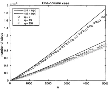
|PI-r| < 2 -, where P' is the transition table and -r' is the stationary distribution of M'.

215 One-column case 2.5 n In(n) 1.8 - 4.5 n In(n) 0 q=2 0 1.6 + q=13 ,V q=251 000 1.4 000 00 -0 1 00O 0.8-E 000 0 0.4 0.2 0 0 1000 2000 3000 4000 5000 n

Figure 3-1: Results of the simulation for the one-column case. The x-axis corresponds to different values of n, while the y-axis shows the value of the variable count, namely the number of steps needed before the Algorithm 1 terminates.

This conjecture implies that the mixing time of the Markov chain M' is O(n ln(n)). As show in the figure, the constant c seems to depend on q: smaller q's (e.g. q = 2) delay the mixing of the chain, because of the bigger probability of cancellation. Nevertheless, even for medium q's (q = 13), the constant c seems to be small enough for our purposes.

3.3.3

One-row case

Similarly to the one-column case, we define M" as the projection of M to one row. We run simulations for the one-row case and count the expected number of steps needed for a single row of the matrix to become uniformly random over GF(q)" \ {₀n}

The pseudocode for this test is shown in 2.

The results of the above simulation for different q's are show in Figure 3-2: Again, we conjecture that:

Conjecture 2. After t O(nln(n)) steps,

I\P"'

- 7r\| < 2-", where P" is the tran-sition table and r" is the stationary distribution of M".

Algorithm 2 One-row case 1: B +- {1, 2,..., n

2: count +- 1

3: A +- In

4: _{row +- a random element in {1, 2, ... , n}} 5: top:

6: if B = 0 then return count

7: pick a random general row operation (i, j, a, b)

8: Ai -- a- Ai+b- Aj

9: count + +

10: if i = row then

11: B +- B \

{k},

Vk such that

A(j,

k)

#

0 12: goto top. x 105 One-row case 2.5 n In(n) 6 n In(n) 2.5 0 q=2 + q=13 2 q=251 2-(D ₀ 00 w0 00 1.5 0 0 500 1000 1500 2000 2500 3000 3500 4000 4500 5000 n

Figure 3-2: Results of the simulation for the one-row case. The x-axis corresponds to different values of n, while the y-axis shows the value of the variable count, namely the number of steps needed before the Algorithm 2 terminates.

Therefore, the mixing time of M" is of the form c - nln(n). However, as show in the figure, in this case c seems to be larger than in the one-column projection when

3.3.4

Expected number of elements equal to

x

c

GF(q)

Another test an adversary can try is to count the number of elements equal to x E

GF(q) in the public matrix A and compare it with the expected number of such

x's in a random invertible matrix. If the two quantities differ significantly, then the adversary knows that the matrix is trapdoored.

Let us define by N() and Nfx) the random variable that shows the number of elements equal to x in a random invertible matrix and trapdoored matrix respectively.

Computing E[N.x)]

If A is a random invertible matrix over GF(q), then by linearity of expectation:

E[N~}

E[ l A,=x]

E3

E[TAijxl

1

i,j<n 1<ij<fl

Each element of A has the same probability of being x. We denote this probability

by px. Then, E[1A3 ] = P.

Since A is an invertible matrix, PX, is the same for every x z 0. So, if we first compute po, then we can find p, from the equation:

pV=

Vx

c

GF(q)

\

{0}

It is well known that the number of invertible matrices with elements in GF(q) is equal to (qrl - 1) - (q' - q) - . (q n - q"n-). Similarly, we can count the number of

matrices in GL(n, q) with the element in position (i,

j)

equal to 0.

Proposition 32. There are (qr-1 - (q" - q) - . (qf - q" 1) matrices in GL(n, q)

with element in position (i, j) equal to 0.

Proof. Without lost of generality, we can assume that i 1. Let A E GL(n, q) with 4ij = 0, then there are (q"- - 1) choices for the n - 1 elements of the first row, since

we exclude the all-zero row. Then, there are q' - q choices for the second row, because

the only limitation is that the second row should not belong to the subspace produces

-Therefore, (q'- -1 - (qn - q) -..- (q" - q"-1) qn-1-1 (qP 1) - (qf -q) ... (qf -qf-1) qf -

1

1_{-o 1 - "-1 "} 1l __=__~ " - q"-1 - ,VxE6GF(q)\{O} q-1 q-1 qn-1 and Computing E[NtP),

Obviously, this expected value depends on the number of steps we have used to create the trapdoor. If this number is large enough, then by the analysis of the previous sections, E[N ] ~zz E[N ].

From the other presented test, we know that we need at least Q(n ln(n)) steps. Therefore, we try to compute the value of E[Nt],] when we have used 0(n ln(n)) steps to create the trapdoor.

Again, by linearity of expectation

E[N

),]

= E[ ( 1Ai = E[1 x] =

>3

q()

_1<it ni,j5n Iij

where A is a trapdoor matrix with trapdoor size L = 6(n ln(n)) and q,) is the probability that Ai, = x.

Also,

=

I

3

E (P

vEGF(q)\{0" } .t.(i)=x < E IP't( vEGF(q)n\{(On} = 211P't(v, -) - 7r'I (vj, v) - 7r'(V)) vj, v) - r'(v)I vj,v) - 7r'(v)I JqX?) p

where vj is the

j-th

basis vector and r' is the stationary distribution of M' (the uniform over GF(q) \ {0"}) and P' its transition matrix.

Therefore, from Conjecture 1:

Jq j - l. <

21-and

|E[N |-

E[Ntjx|

< 2n-1

3.4

Other Trapdoor Constructions

The above candidate construction is not the only one that can be used in the protocol. It is possible that picking the rows i and

j

in each step randomly delays the mixing of the Markov chain. There are examples of Markov chain where we see this behavior. For instance, in the case of random walks on upper triangular matrices, the mixing time is 0(n2 _{log(n)) when the generator set is {A : A elementary matrix corresponding}

to row operation A <- Ai

+

b - A, where i <

j

and b E GF(q)} [171, but it is 0(n 2 log(q)) when the generator set is {A : A elementary matrix corresponding to row operation Ai - A + b - A_1, where b E GF(q)} [181.

So, another possible construction could be the following:

For k E 1... L(n):

" Pick

jA

uniformly at random from {1,.. ., n} \ {(k - 1) mod n, k mod n} " Pick ak uniformly at random from GF(q) \ {O}

" Pick bk uniformly at random from GF(q)

" Pick ck uniformly at random from GF(q)

Then,

where A(k) is the corresponding to the operation Ak mod n -- ak -A(k mod n) + bk * A(k-1 mod n)+ Ck -Aj. Each A(k) can be written as a product of two general elementary matrices.

Thus, the trapdoor T(A) consists of the sequence of L(n) tuples:

(Uk, ak, bk, Ck), for k = 1, 2,..., L

The program, that the honest party uses, takes advantage of the knowledge of the trapdoor and is similar to the one presented previously.

We notice that in the case of very large q, 2n steps are enough for the mixing of the one-column case. However, similar experiments to the random case show that this might not be true for small q's. Therefore, since we have no additional theoretical analysis for this construction, we focus our attention to the previous one.

Chapter 4

Implementation in practice

In this chapter, we consider the practicality of the protocol. We give the basic char-acteristics of a smart card and based on them we specify the values that the protocol parameters can get.

4.1

Characteristics of smart cards

In order to judge the implementability of our protocol, we provide some of the tech-nical characteristic of a specific smart card [16].

The P60D080 and P60D144 devices are members of the new SmartMX2 Family produced by NXP. Their basic features:

* EEPROM: choice of 80 KB or 144 KB

" ROM: 384KB

" RAM: 8.125 KB (8320 B)

- 5632 B CXRAM (including 256 B IRAM) usable for CPU - 2688 B FXRAM usable for Fame2 or CPU

" SmartMX2 CPU: orthogonal instruction set offering 32-/24-/16-/8-bit

* ISO/IEC 7816 contact interface (UART) and ISO/IEC 14443A Contactless In-terface Unit (CIU)

- ISO/IEC 7816 contact interface (UART) offering hardware support for

ISO/IEC 7816 T = 0 and T = 1 protocol stack implementation

- ISO/IEC 14443A Contactless Interface Unit (CIU) supporting data rates

of 106 kbit/s, 212 kbit/s, 424 kbit/s, 848 kbit/s and offering hardware support for ISO/IEC 14443 T = CL protocol stack implementation

4.2

Suggestions on the protocol parameters

We suggest that we need at least one order of magnitude difference on the time the prover, with her trapdoor, needs to spend to perform the computation and the time any other adversary, without the trapdoor, would need. Simultaneously, we need to be sure that n is not too large to be practical. The use of this protocol in smart cards sets also constrains on the parameters. For example, smart cards have limited space, so the trapdoor must be designed so that it offers a significant advantage to the prover, even in the case that she can use limited space to perform the computation.

We have implemented the naive algorithm for matrix-vector multiplication and the algorithm that uses the trapdoor information in Matlab in order to estimate the size of the parameters of the protocol. We have tested both the constructions of the previous chapter, but since the results are very similar, we present only those of the first construction. In this construction, the trapdoor is a sequence of random elementary matrices.

The parameters of our protocol are:

* q, the size of the finite field, GF(q), over which all operations are done. In the

implementation, we try three different values of q, a small one (2), a medium

(13) and a sufficiently large (251). Smarts cards have limited space, so we limit q so that each element is at most one byte.