DOI 10.1007/s10584-010-9931-5
Irrigation as adaptation strategy to climate
change—a biophysical and economic appraisal
for Swiss maize production
Robert Finger· Werner Hediger · Stéphanie Schmid
Received: 18 December 2008 / Accepted: 14 June 2010 / Published online: 24 September 2010 © Springer Science+Business Media B.V. 2010
Abstract The impact of climate change on Swiss maize production is assessed using an approach that integrates a biophysical and an economic model. Simple adaptation options such as shifts in sowing dates and adjustments of production intensity are considered. In addition, irrigation is evaluated as an adaptation strategy. It shows that the impact of climate change on yield levels is small but yield variability increases in rainfed production. Even though the adoption of irrigation leads to higher and less variable maize yields in the future, economic benefits of this adoption decision are expected to be rather small. Thus, no shift from the currently used rainfed system to irrigated production is expected in the future. Moreover, we find that changes in institutional and market conditions rather than changes in climatic conditions will influence the development of the Swiss maize production and the adoption of irrigation in the future.
1 Introduction
Climate change is expected to affect agriculture in different ways and to a different extent in different parts of the world and in different agro-ecosystems (Olesen and Bindi2002; Parry et al.2004). The consequences will depend on local climatic and soil conditions, on the political and economic framework, and on the farmers’
R. Finger (
B
)Agri-food and Agri-environmental Economics Group ETH, Sonneggstrasse 33, 8092, Zürich, Switzerland
e-mail: [email protected] W. Hediger
Swiss College of Agriculture SHL, Laenggasse 85, 3052, Zollikofen, Switzerland S. Schmid
Agroscope Reckenholz-Tänikon Research Station ART, Reckenholzstrasse 191, 8046, Zürich, Switzerland
management and adaptation decisions. The latter entail several options to cope with climate change on the field and farm level (see, for instance, Risbey et al.1999; Smit and Skinner2002). Apart from agronomic aspects, these options involve economic decisions taken by individual farmers who optimize their production by adapting their use of fertilizers, pesticides and irrigation water to changing climatic, political and economic conditions.
The goal of this study is to analyze impacts of climate change on the maize produc-tion at the Swiss Plateau taking different climate and price scenarios into account. We consider two simple adaptation options on the field level: (a) shifts in sowing dates and (b) changes in the production intensity. Building on this background, we further evaluate irrigation as a strategy to cope with climate change.
The Swiss Plateau is the major production region for cereals in Switzerland. Changes in climatic conditions in this region are expected to particularly affect the production of spring-sown cereals such as maize. Due to elevated temperatures and reduced summer rainfalls, maize yields might be considerably reduced and become more variable if no adaptation measures are taken (Torriani et al.2007a,b). Using a crop simulation model, Torriani et al. (2007a) evaluated different adaptation strate-gies for the Swiss maize production. Their analysis shows that earlier sowing, changes in thermal requirements (i.e. breeding) and irrigation can compensate (or even over-compensate) climate change induced effects on yield levels and yield variability.
Some adaptation options such as shifts in sowing dates might be implemented without costs for the farmers. Other options such as the implementation of irrigation farming involve costs and thus require an assessment that is also based on economic grounds. To examine this problem, we apply an approach that integrates biophysical and economic modeling. This particularly facilitates the analysis of the combined effects of future changes in climate and agricultural prices on optimal yield levels, yield variability and the economic benefits of irrigation systems. In contrast to other approaches that analyze potential crop yields or production systems under unadapted management conditions, our approach compares crop yields under cur-rent and future climatic conditions that take into account the management decisions by the farmer (see Finger and Schmid 2008, for a discussion on other modeling approaches).
The current situation shows that only about five percent of the cultivated acreage in Switzerland is irrigated. It is mainly located in alpine dry valley regions and used to the largest extent in grassland, vegetables, vine and fruit production. In contrast, cereals are currently irrigated only to a very small extent (Weber and Schild2007). However, climate change is expected to increase the agricultural water demand. As a consequence, competition for water among ecosystems and different economic sectors such as industry and agriculture is expected to increase in the future (Bates et al.2008; OcCC2007,2008). Therefore, the analysis of the potential of irrigation as an adaptation option in Swiss cereal production is crucial for the optimal future design of agricultural extension as well as policy measures that support farmers’ adaptation to climate change and environmental protection.
According to previous results (Finger and Schmid 2008), climate change is ex-pected to have small positive effects on winter wheat production, which represents the majority of the Swiss cereal production. Moreover, irrigation is expected to lead neither to significantly higher winter wheat yield levels nor to economic benefits in changed climatic conditions because relevant spring rainfalls are expected to
decrease only slightly (Finger and Schmid2008; Torriani et al.2007a). The present analysis is therefore focused on maize that is the most important spring-sown cereal and covers about 12% of the total cereal production acreage (SBV 2006). Globally, maize is one of the most important cereals for human and animal nutrition. Accordingly, it will be important to have analyses of climate change impacts on maize production and potential adaptation strategies in different parts of the world. Our analysis might particularly indicate the direction of climate change impacts on maize production and consequences for agricultural water demand in other Middle-European regions that face similar climatic and production conditions.
2 Data and model description
In the following section, we present our modeling approach that integrates a bio-physical and an economic model. The biobio-physical model is used to simulate yield responses to the crucial agricultural inputs nitrogen fertilizer and irrigation water in current and future climatic conditions. In the economic model, input use is optimized in order to maximize farmers’ certainty equivalents of the farmer’s quasi-rent. This approach takes into account both yield levels and yield variability. To link the bio-physical simulation and the economic optimization model, crop production and yield variation functions are estimated.1
2.1 Biophysical model and climate scenarios
We use the deterministic crop yield simulation model CropSyst to mimic the relation-ship between maize yields and input use for current and future climatic conditions. It models above- and below-ground processes (e.g. the soil water budget, soil–plant nitrogen budget, crop phenology, canopy and root growth, and crop yield) on a daily time step (see Stöckle et al.2003, for details). In CropSyst, these processes are simulated in response to crop and soil characteristics, daily weather data, and management options.2
In this study, we consider current climate conditions as well as three different sce-narios of climate change. To represent current climate conditions, we use weather data from meteorological stations at the eastern Swiss Plateau for the years 1981 to 2003. The three climate change scenarios in our analysis are taken from Frei (2005), whose projections were performed within the scope of the PRUDENCE project (Christensen et al.2002) on the basis of simulations with 16 different scenario–model combinations.3 The climate projections used in this study represent the median of these ensemble simulations for the years 2030 and 2050 plus the 97.5% percentile for the year 2050. These scenarios are tagged in the following as 2030, 2050 and 2050X.
1More detailed descriptions and discussions of the modeling approach are given in Finger and Schmid (2008) and Torriani et al. (2007a).
2Model calibration and settings for maize production at the Swiss Plateau are presented in Torriani et al. (2007a).
3The simulations conducted by Frei (2005) included two emission scenarios, four global climate models as well as eight regional climate models.
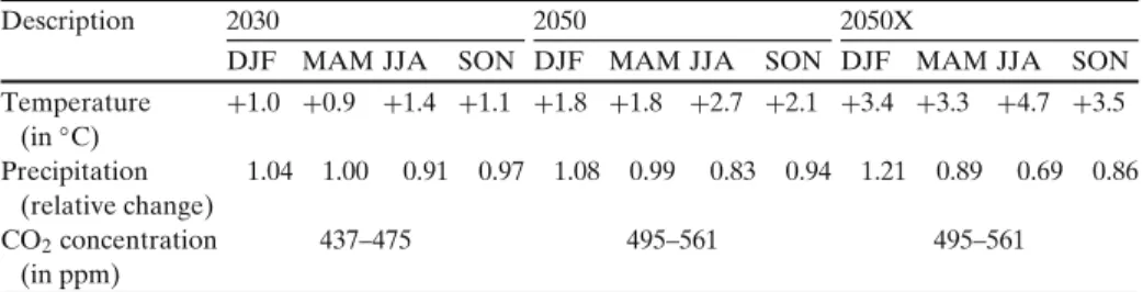
Table 1 Description of climate scenarios
Description 2030 2050 2050X
DJF MAM JJA SON DJF MAM JJA SON DJF MAM JJA SON Temperature +1.0 +0.9 +1.4 +1.1 +1.8 +1.8 +2.7 +2.1 +3.4 +3.3 +4.7 +3.5 (in◦C) Precipitation 1.04 1.00 0.91 0.97 1.08 0.99 0.83 0.94 1.21 0.89 0.69 0.86 (relative change) CO2concentration 437–475 495–561 495–561 (in ppm)
Scenarios for Northern Switzerland. CO2concentrations for the base scenario range from 339 to
379 ppm. CO2concentrations vary randomly within the defined range for each climate scenario
Source: IPCC (2000) and Frei (2005)
DJF December–February, MAM March–May, JJA June–August, SON September–November
The last scenario represents a rather extreme assumption of climate change, whereas the first two scenarios assume moderate changes in climatic conditions (Table1).
Based on today’s weather data and the anomalies of temperature and precipita-tion, sets of future weather data are generated using the stochastic weather generator LARS-WG (Semenov et al.1998). To enable meta-modeling analysis and avoid dis-tortions due to dynamic effects, all simulations are conducted using identical starting conditions. We assume a representative soil for the Swiss Plateau that is character-ized by a texture with 38% clay, 36% silt, 26% sand, as well as by a soil organic matter content at 2.6% weight in the top soil layer (5 cm) and 2.0% in lower soil layers.
Sowing dates and expected dates of maturity are given in Table2. For the climate change scenarios, we used earlier sowing dates because this reduces negative effects of climate change such as increased heat and drought stress. As a consequence of increased temperatures, maturity periods are shorter in the climate change than in the Base scenario. Thus, sowing and harvesting dates as well as the length of the maturity period are expected to change considerably in the future.
The management scenarios for the CropSyst simulations include application of nitrogen and irrigation water. Depending on the applied amount of nitrogen, three to four fertilizer applications are made at different stages of the cropping season. The annual amount of applied nitrogen ranges from 0 to 320 kg ha−1. To simulate irrigation, we chose the automatic irrigation option of CropSyst. Thus, irrigation is triggered as soon as soil moisture is lower than a specific user-defined trigger value. The degree of soil moisture is expressed as a value between 0 (permanent wilting point) and 1 (field capacity). When soil moisture falls below the previously defined
Table 2 Sowing and expected maturity dates
Climate scenario Base 2030 2050 2050X
Sowing date 10th May (130) 7th May (127) 4th May (124) 30th April (120) Expected day of 17th September 4th September 28th August 18th August
maturity (263) (250) (240) (230)
Expected length of 133 123 116 110
maturity period (days)
Numbers in brackets are days of year. Sowing dates for current and future climate follow Dubois et al. (1999) and Torriani et al. (2007a). Expected days of maturity are derived from CropSyst simulations
value, water is added to the soil until field capacity is reached with an upper limit of 20 mm per irrigation event. For each year, one simulation is conducted without application of fertilizer and irrigation. Furthermore, to set up an experimental design, the amount of fertilizer and the value that triggers irrigation was varied randomly. To allow for comparability of the results, the simulated experimental framework is equal for each climate scenario. This data simulation leads to individual data sets for the different climate scenarios that contain information of maize yield and the amount of applied input for each observation.4
2.2 Production and yield variation functions
This output from the biophysical simulation is used to estimate production and yield variation functions. These functions are simple analytical descriptions of yield and yield variability responses to nitrogen and irrigation, which are used to integrate these biological response processes in the economic allocation model. Thus, the esti-mated functions are the linkage between the biophysical model and the economic model. The per-hectare production function, Y = f (N, W), is fitted to a square root functional form:5
Y= α0+ α1· N1/2+ I · α2· W1/2+ α3· N + I · α4· W + I · α5· (N, W)1/2 (1) Y denotes maize yield (kg ha−1), N the amount of nitrogen applied (kg ha−1), W the irrigation water applied (in mm), and I is an indicator to distinguish rainfed(I = 0) and irrigated (I = 1) farming systems. The αi’s are parameters that must satisfy the subsequent conditions to ensure decreasing marginal productivity of each input factor: α1, α2> 0 and α3, α4< 0. Furthermore, if α5> 0, the two input factors are complementary. They are competitive if α5< 0, while α5= 0 indicates independence of the two input factors.
In order to take the effect of input application on both yield and yield variability into account, we use a Just and Pope (1978,1979) production function that allows inputs to influence both the mean and the variance of output:
Y= f(N, W) + h(N, W)ε (2)
f(N, W) and h(N, W) denote the production and yield variation function, respec-tively, and we assume E(ε) = 0 and σ (ε) = 1. Thus, f (N, W) and h(N, W) represent the expected yield level and the standard deviation of maize yields (σY(N, W)), respectively. Following Koundouri and Nauges (2005), we estimate this function in two steps. Firstly, the production function coefficients are estimated and the associated residuals are computed( ˆw = Y − ˆY). In a second step, the absolute values of these residuals are used to estimate the yield variation function. Thus, yield variation,σY(N, W), is defined as the absolute difference between observed yields (i.e. yields simulated with CropSyst) and expected yields (i.e. yield values on the
4Depending on the climate scenario, these data sets contain between 527 and 531 observations. Data sets are available from the authors upon request.
5The selection criteria for the applied functional forms and the estimation methodology are described in Finger and Hediger (2008) and Finger and Schmid (2008).
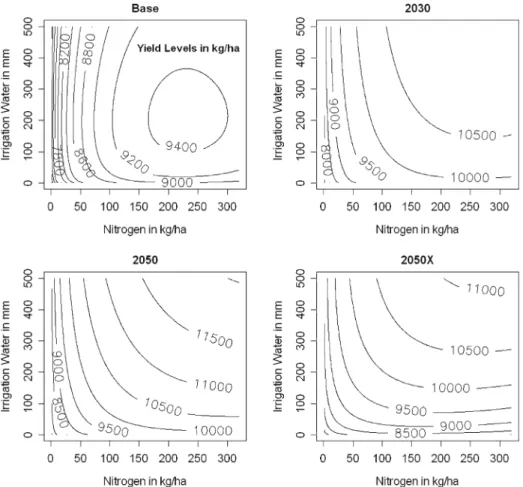
Fig. 1 Contour plots of the production functions: crop yield as function of nitrogen and irrigation
water
production function) in our analysis. The following specification is used to estimate the relationship between yield variability and input use:
σY(N, W) = β0+ I · β1· W0.5+ β2· N0.5 (3) Shifts in the intercept,β0, capture effects of changes in weather conditions on yield variation across different climate scenarios.β1sandβ2quantify the influence of irri-gation and nitrogen application on yield variation. An input is risk decreasing if βi< 0 and risk increasing if βi> 0, respectively.
For each climate scenario, a single production and yield variation function is esti-mated. The estimation results6of these functions are presented as contour plots in Figs.1and2.
Contour plots (i.e., isoquants) for the production functions show that future maize yields, ceteris paribus, exceed current levels (Fig. 1). For constant levels of
Fig. 2 Contour plots of the yield variation functions: crop yield variability as function of nitrogen
and irrigation water
nitrogen application without irrigation, yield levels increase from the Base to the 2050 scenario, but decrease from the 2050 to the 2050X scenario. Increasing yield levels are caused by higher CO2 concentrations and the applied shifts in sowing date. For the 2050X scenario, temperature increases and reductions in the amount of summer rainfall offset the benefits of increased CO2 concentrations. Moreover, it shows that irrigation water becomes a more important production factor in the future. In current climatic conditions, the crop yield response to irrigation water is small because water is no limiting factor in maize production at the Swiss Plateau. Increasing temperatures and lower amounts of summer rainfall in the climate change scenarios reduce the water available to the plant and thus increase the yield responses to irrigation water. While crop yields are nearly independent from irrigation water in the Base scenario, the production factors nitrogen and irrigation water become more complementary in the climate change scenarios. This indicates that future maize yields might exceed current levels if sufficient water availability is ensured by supplemental irrigation.
In Fig. 2, contour plots of the yield variation functions are presented. It shows that nitrogen application increases, but irrigation reduces, ceteris paribus, yield
variability. Moreover, climate change increases yield variability. For constant levels of nitrogen application without irrigation, yield variability increases from the Base and 2030 scenarios to the 2050 and 2050X scenarios. However, the propensity of irrigation to reduce maize yield variability increases from the Base to the 2050X scenario because increases in the applied amount of irrigation water lead to larger reductions of yield variability in the climate change scenarios than in the Base scenario. Thus, expanded application of irrigation might counteract climate changed induced increases of yield variability in the future.
2.3 The economic model
The production and yield variation functions are integrated in the economic model to derive the optimal input allocation for different climate scenarios. To this end, the economic model is based on the maximization of the certainty equivalent (CE).7 This is a certain level of payoff which provides a (risk averse) decision maker with the same benefit as a higher but uncertain level of payoff, and is defined as follows:
CE= E(π) − RP (4)
Where E(π) is the expected quasi-rent π (revenue minus variable costs) and RP is the risk premium, which is the difference between the expected quasi-rent and the certainty equivalent. The expected quasi-rent is defined as:
E(π) = pE(Y(N, W)) − ZNN− ZWW (5)
Where ZN and ZW stand for the input prices for nitrogen N and irrigation water
W, respectively, p stands for the output (maize) price, and Y(N, W) denotes the production function.
Following Di Falco et al. (2007) and Pratt (1964), we define the risk premium in our analysis as RP= 0.5 γ σ2
π/E(π). Where γ is the coefficient of relative risk
aversion. We choose constant coefficient of relative risk aversion (CCRA), equal to 2, that represents a typical (moderate) form of risk averse behavior and implies decreasing absolute risk aversion (Di Falco and Chavas 2006). By focusing on the variability of production and assuming constant price levels, the variance of the quasi-rent can be expressed as follows: σ2
π= p2σY2(N, W), where σY(N, W) is the
standard deviation of maize yields. Accordingly, our optimization problem is defined as follows:
max
N,W CE= E(π(N, W)) − 0.5 γ p 2σ2
Y(N, W)/E(π(N, W)) (6)
The certainty equivalent is maximized subject to the production function constraint Y= f (N, W). Input prices are restricted to variable costs. Thus, total variable costs are defined as the variable nitrogen costs (nitrogen applied x nitrogen price) plus the variable irrigation costs (irrigation water applied x irrigation water price). Other costs are assumed constant and thus irrelevant for the optimal input combination.
7General discussions on the certainty equivalent maximization approach, the here used methodology and underlying assumptions are given, for instance, in Chavaz (2004), Di Falco and Chavas (2006), and Pratt (1964).
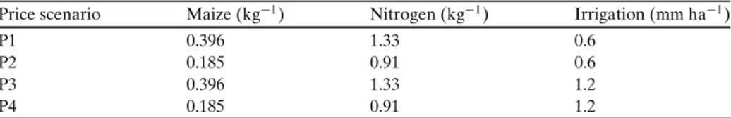
Table 3 Price scenarios (in CHF)
Price scenario Maize (kg−1) Nitrogen (kg−1) Irrigation (mm ha−1)
P1 0.396 1.33 0.6
P2 0.185 0.91 0.6
P3 0.396 1.33 1.2
P4 0.185 0.91 1.2
Current price levels for maize and nitrogen in Switzerland and the EU refer to the year 2006, following Hartmann et al. (2007) and Finger and Schmid (2008)
To compare irrigation and rainfed farming, Eq.6is solved for both irrigation and non-irrigation farming independently. If rainfed farming is assumed, production and yield variation functions only contain nitrogen but no irrigation water. The farmer’s economic benefit of the adoption of irrigation farming, expressed in monetary values, is the difference between optimal (i.e. maximum) certainty equivalents for irrigated farming, CE∗(I = 1), and rainfed farming, CE∗(I = 0):
DCE= CE∗(I = 1) − CE∗(I = 0) (7)
This measure is used in our analysis to assess the expected relative advantage of irrigation farming.
2.4 Price scenarios
In order to derive optimal levels of input, output and utility, information about input and output prices is required. Current price levels and price scenarios for maize, nitrogen and irrigation water are given in Table3.
In the price scenario P1 all price levels are assumed to remain on current levels. Because this implies agricultural prices that are much higher in Switzerland than in other European countries, we additionally employ the price scenario (P2) that assumes current maize and nitrogen prices observed in the European Union. This scenario reflects expected decreases in price levels if market liberalization, e.g. with the European Union, takes place.
Furthermore, we combine these two price scenarios with the assumption of higher water prices caused, for instance, by higher withdrawal fees or increasing use of ground- instead of surface water in the future. In drought years, as it was the case in 2003, access to surface water might be restricted and groundwater has to be used instead, leading to higher withdrawal fees and pumping costs (ProClim2005). This combination of a higher water price with the two price scenarios P1 and P2 leads to the scenarios P3 and P4 (see Table3). In addition, we provide a sensitivity analysis in assessing the effect of different water prices on the on-site economic benefits of irrigation farming as well as on the optimal amount of irrigation water.
3 Results and discussion
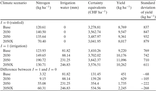
For the price scenario P3, Table4 shows optimal factor inputs, yield levels, yield variation, coefficients of variation and certainty equivalent income levels for both rainfed and irrigated farming under different climate conditions—i.e., for the Base scenario and the 3 climate change scenarios. It shows increasing yield levels for both
Table 4 Optimal input levels, certainty equivalents, yields and yield variation
Climate scenario Nitrogen Irrigation Certainty Yield Standard (kg ha−1) water (mm) equivalents (kg ha−1) deviation
(CHF ha−1) of yield (kg ha−1) I= 0 (rainfed) Base 120.61 0 3,278.81 8,769 837 2030 140.50 0 3,562.74 9,547 847 2050 135.64 0 3,487.97 9,361 932 2050X 70.40 0 3,041.95 8,017 879 I= 1 (irrigation) Base 123.93 81.82 3,410.26 9,220 769 2030 149.65 88.14 3,702.02 10,176 742 2050 190.72 231.25 3,842.37 11,096 710 2050X 130.71 246.83 3,576.51 10,262 611
Difference between I= 1 and I = 0
Base 3.32 81.82 131.45 451 −68
2030 9.15 88.14 139.28 629 −105
2050 55.08 231.25 354.4 1,735 −222
2050X 60.31 246.83 534.56 2,245 −268
The price scenario reported is P3. The coefficient of variation is calculated as the ratio of the yield variation and the yield level. 2030, 2050, 2050X denote the climate scenarios described in Table1
irrigated and rainfed farming from the Base to the 2030 scenario. Thereafter, yield levels are expected to decrease in rainfed farming systems. In particular, the yield level in the 2050X scenario is expected to be considerably below the current level. Moreover, the relative yield variability (i.e. the coefficient of variation) in rainfed production systems is expected to increase with more pronounced climatic changes.
In irrigation farming systems, future yields are expected to be above current levels because climate change provides an economic incentive to expand irrigation activities. Furthermore, increases in the optimal amount of applied irrigation water reduce yield variability in the future. As a consequence, also relative yield variability is expected to decrease in irrigated maize farming systems.
A comparison of optimal input levels of nitrogen between rainfed and irri-gated farming systems reveals different adaptation strategies. In rainfed production systems, reduced summer rainfalls lead to a reduction of the optimal production intensity from the Base and the 2030 scenarios to the 2050 and 2050X scenarios. In contrast, an increased application of nitrogen, i.e. a more intensive production, is an optimal response to climate change if irrigation is available.8
By integrating the possibility to adjust production intensity, our modeling ap-proach avoids the overestimation of economic losses due to climate change. Even though optimal yield levels and yield variations between irrigated and rainfed farming systems considerably differ for the climate change scenarios, the differences in certainty equivalents between those farming systems remain relatively small (Table4).
8Adaptation strategies towards more intensive production by increasing nitrogen application might be limited in practice due to cross compliance components in agri-environmental policy.
a) Rainfed Maize Production
Changes in Yield Levels (%)
-10 0 1 0 2 0 3 0 4 0 2030 2050 2050X P1 P2 P3 P4 Climate Scenarios Price Scenarios
Changes in Yield Variability (%)
-40 -30 -20 -10 0 1 0 2 0 2030 2050 2050X CV = 0.09 0.08 0.09 0.08 0.10 0.10 0.10 0.10 0.11 0.11 0.11 0.11
b) Irrigated Maize Production
Changes in Yield Levels (%)
-10 0 1 0 2 0 3 0 4 0 2030 2050 2050X Climate Scenarios Price Scenarios P1 P2 P3 P4
Changes in Yield Variability (%)
-40 -30 -20 -10 0 1 0 2 0 2030 2050 2050X CV = 0.06 0.07 0.07 0.08 0.05 0.06 0.06 0.08 0.05 0.06 0.06 0.07
Fig. 3 Relative changes to the base scenario: yield levels, absolute and relative yield variability for
three climate change and four price scenarios. Changes are relative to the base scenario. CV denotes the coefficient of variation. 2030, 2050, and 2050X denote climate- and P1–P4 denote price scenarios that are described in Tables1and3, respectively
Expected changes, relative to the Base scenario, in yield levels and yield variability for all price scenarios are summarized in Fig.3. In rainfed production, yield levels are higher in the 2030 and 2050 scenarios but lower in the 2050X scenario. Moreover, yield variability is expected to increase for almost all scenarios.9 However, the expected increase in relative yield variability is relatively small. The coefficient of variation (CV) increases, in maximum, from 0.09 in the base to 0.11 in the 2050X scenario. A higher maize price (comparing the P1 and the P2 price scenario) leads to higher yield levels and higher yield variability as the optimal amount of nitrogen application is augmented.
For irrigated maize production, future yield levels are expected to increase and yield variability is expected to decrease for all price scenarios. As previously dis-cussed for the yield variation functions, irrigation becomes more important in coping
9No differences between the scenarios P1/P3 and P2/P4 exist for rainfed production because water prices are not relevant.
with the climate change induced increases of farming risk. Moreover, the optimal amount of irrigation water increases for climate change scenarios due to an increasing evapotranspiration as well as due to the fact that irrigation water and nitrogen be-come more complementary with climate change (Fig.1). Thus, climatic changes lead to higher incentives for the expansion of irrigation activities that increase, ceteris paribus, yields and decrease yield variability. However, it shows that the results for irrigated farming are highly sensitive to changes in price levels. A decreasing maize price (comparing P1 and P2) as well as an increase of the water price (comparing P1/P3 and P2/P4) reduce the incentives to expand irrigation activities and thus result in smaller yield increases and smaller decreases of yield variability.
These results are in line with other studies for Europe: climate change is expected to lead to small increases in the productivity of crops, particular in north- and middle European regions—however, climate change might also increase agricultural production risks (for overviews see Alcamo et al.2007, and Olesen and Bindi2002). In order to analyze whether the increasing differences in yield levels and yield variability between irrigated and rainfed maize production might result in a frequent adoption of irrigation farming systems in the future, differences in certainty equiva-lents (DCE) are analyzed (see Eq.7). These differences reflect the expected annual economic benefits enabled by the adoption of irrigation farming. The DCE increases constantly from the 2030 to the 2050X scenario for all price scenarios, as shown in Fig.4.
Differences in Certainty Equivalents (DCE) in CHF/ha
0 200 400 600 800
Base
2030
2050
2050X
Climate Scenarios Price ScenariosP1
P2
P3
P4
DCE relative to CE (rainfed): 4% 6% 4% 4% 2% 17% 9% 10% 5% 24% 16% 18% 10%Fig. 4 Absolute and relative differences of certainty equivalents between irrigated and rainfed maize
farming. Relative differences are given in percent of the certainty equivalents in rainfed production. 2030–2050X denote climate and P1–P4 denote price scenarios that are described in Tables1and3, respectively
For the price scenario P1, future DCEs exceed the current value considerably. Higher temperatures and reductions of summer rainfalls increase, ceteris paribus, the profitability of irrigation in maize farming. However, reduced output prices (scenario P2) as well as higher water prices (P3, P4) result in much smaller expected rises in DCE. Especially for the price scenario P4, which assumes a low maize but high water price, future DCEs exceed current levels only for the 2050X scenario. The ratio of future DCEs to the corresponding certainty equivalents in rainfed production, range between 2% and 24% and increase constantly from the 2030 to the 2050X scenario.
In our modeling approach, estimated economic benefits of irrigation farming are already reduced by considering other adaptation options, i.e. shifts in sowing dates and changes in production intensity.
To compare the estimated benefits with the cost of the adoption of irrigation farming we consider cost calculations of 3 irrigation projects at the Swiss Plateau that have been recently realized.10These calculations show annual fixed costs (amor-tization, maintenance, etc.) of irrigation systems between about 800 and 2,000 CHF per hectare and year.11They are highly sensitive to the assumed asset depreciation rates, which might be larger in practice than assumed in our assessment.12Moreover, the effective adoption costs will be heterogeneous among irrigation projects due to differences, for instance, in farm size, soil and farm characteristics, access to irrigation water as well as infrastructure endowments (Kulshreshtha and Brown1993; Negri et al.2005). Thus, the above estimates of annualized fix costs indicate that the adop-tion costs the most likely exceed the estimated economic benefit for current as well as future climatic conditions (cf. Fig.4). As a consequence, our results suggest that future adoption rates of irrigation in maize farming systems will remain small even in changed climatic conditions.
This result can be relevant for other cases of agricultural adaptation to climate change: Even though irrigation seems to be a promising adaptation option to avoid yield reductions and increases in yield variability in the face of climate change (e.g. Akpalu et al. 2009; Fuhrer and Jasper 2009; Fuhrer et al. 2006; Mendelsohn and Dinar2003; OcCC2007,2008; Rosegrant et al.2009; Torriani et al.2008), it might not necessarily be economic viable.
The development of governmental support (e.g. share of covered costs, allocation practice) will also be a key driver of farmers’ adoption decisions in the future. At present, up to 50% of the adoption costs for an irrigation system can be covered by national and cantonal bodies.13 However, the current practice of these support payments at the Swiss Plateau is restrictive and focused on cooperative projects. Altogether, our results indicate that the future demand for irrigation water in Swiss maize production might be determined by the development of price levels and governmental support rather than by climate change.
10Personal communication Andreas Schild, Swiss Federal Office for Agriculture, Bern.
11Current water withdrawal fees range from unique user fees to annual fees and differ considerably across cantons, both with respect to the level of fees and the period that is charged for (Weber and Schild2007).
12The assumed asset deprecation period is 10 years for mobile equipment such as motors and pumps, and 15 years for fixed installed equipment such as pipelines.
13In addition, investment loans—free of interest—are provided by the Swiss Federal Office for Agriculture to partially finance the remaining investment costs.
Relative Change in Water Price (in % from 0.06 CHF/m3)
Differences in Certainty Equivalents (in CHF/ha)
-50% -25% 0% +25% +50% +75% +100% +125% +150% +175% +200% +225% +250% 100 200 300 400 2030 2050 2050X Climate Scenarios
Relative Change in Water Price (in % from 0.06 CHF/m3)
Optimal Amount of Irrigation Water (mm per ha)
-50% -25% 0% +25% +50% +75% +100% +125% +150% +175% +200% +225% +250% 150 300 450 600 2030 2050 2050X Climate Scenarios
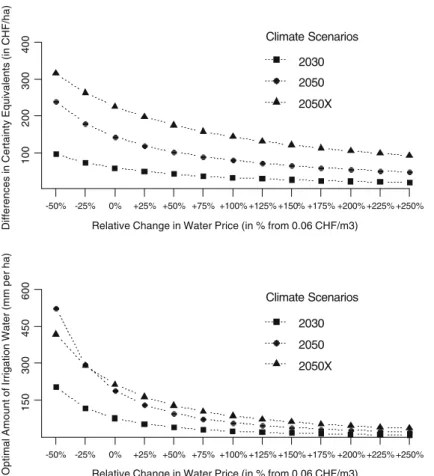
Fig. 5 Sensitivity analysis: changing water prices. Calculations are based on price scenario P2. 2030,
2050 and 2050X denote climate scenarios that are described in Table1
Finally, the future profitability of irrigation and the demand for irrigation water in maize farming systems are expected to be sensitive to water prices. To analyze these sensitivities, we show in Fig.5the DCE levels and the optimal amounts of irrigation water for different water prices. Assuming current EU prices for maize and nitrogen (price scenario P2), we vary the water price stepwise in a range of−50% to +250% of the current level. Higher water prices might reflect enhanced competition for water among different economic sectors or an intensified use of ground-water. Moreover, higher withdrawal fees might reflect the internalization of negative externalities such as, for instance, water pollution from nutrients and pesticides, habitat damages by abstraction of water as well as impacts on quantity and quality of soils (Baldock et al.
2000).14In contrast, decreasing withdrawal prices might reflect further subsidization of pumping costs by providing support to electricity or fuel costs.15
14In Switzerland, potential environmental damages of irrigation are limited to some extent due to strict obligations in agricultural cross compliance measures as well as in the bill on water protection. 15Currently, Swiss farmers are partially exempted (via reimbursement) from fuel taxes.
Figure5shows that decreasing water prices result in an over-proportional increase of the privately optimal amount of irrigation water applied per hectare. In contrast, increasing water prices gradually offset higher certainty equivalent levels in irrigated vis-a-vis rainfed maize production for all climate scenarios. In addition, the optimal amount of irrigation water sharply decreases for higher water prices. Thus, increasing water prices might outweigh climate change induced incentives for the adoption of irrigation in Swiss maize farming.
In contrast, the analysis of farmers’ reactions to increasing irrigation water prices given in other studies show much more moderate irrigation water demand elasticities than indicated by our sensitivity analysis. In particular for low water prices, farmers’ water demand may be much more influenced by other determinants—such as agri-cultural policy, product prices, and structural factors—than by the water price, (Garrido 1999; Gómez-Limón and Riesgo 2004). Moreover, higher water prices do not necessarily result in reduced water demand because farmers change their management practice (e.g. adjusting the timing of operations) and cropping patterns (e.g. using crops with lower water requirements) instead. Water price increases might even lead to—counterintuitive—increases in the water demand. Higher water prices can induce the adoption of more efficient irrigation technologies that increase marginal benefits of water use and thus increase the water demand (Garrido1999).
We are aware that risk attitudes can differ between farmers and over time, in par-ticular in presence of agricultural policy reforms (e.g. Koundouri et al.2009). Thus, it is necessary to conduct sensitivity analysis also with regard to the assumed parameter of relative risk aversion. To this end, we analyze the effect of changes in the coeffi-cient of relative risk aversion in the range of 0 to 4 (assuming price scenario P1), which represents risk neutral farmers and typical forms of risk behavior (Di Falco et al.2007), on the differences in certainty equivalents between irrigated and rainfed conditions as well as on the optimal amount of irrigation water applied per hectare. The results of this sensitivity analysis are displayed in Fig.6. It shows that increasing risk aversion leads to increases in the optimal amounts of irrigation water applied as well as increasing differences in certainty equivalents between irrigated and rainfed conditions. Thus, as expected, more risk averse farmers use more irrigation water and have higher incentives for the adoption of irrigation farming. However, in the here presented analysis price changes (e.g. Fig.5) tend to have a larger influence on the results than changes in risk attitudes.
The here presented analysis is focused on the mean and variability of yields. However, both input use and climate change might also affect higher moments of crop yield distributions. Thus, further research should also account for downside risk aversion (see e.g. Di Falco and Chavas 2006) and the potential impact of climate change on the skewness of crop yield distributions.
In our model, water is assumed to be allocated perfectly, without any losses, for instance, due to runoff. Depending on the irrigation system (e.g. flood-, sprinkler-, or drip-irrigation), the water use efficiency of irrigation (i.e. the ratio of net irrigation water and the amount of water that has to be withdrawn) might be substantially smaller in reality than our implicitly assumed value of 1 (cf. Zilberman et al.1997). Hence, the marginal productivity and thus the economic benefits of irrigation are overestimated in our model. Moreover, short and long-term on-farm damages of irrigation such as salinization, nutrient leaching or erosion are not considered in our model. In other words, the dynamic processes of irrigation-induced losses of
Fig. 6 Sensitivity analysis:
changing coefficients of risk aversion. Calculations are based on price scenario P1. 2030, 2050 and 2050X denote climate scenarios that are described in Table1
Coefficient of Relative Risk Aversion
Differences in Certainty Equivalents (in CHF/ha)
0 0.5 1 1.5 2 2.5 3 3.5 4 200 400 600 800 200 400 600 800
Optimal Amount of Irrigation Water (in mm per ha)
2030 2050 2050X Climate Scenarios:
Differences in Certainty Equivalents Optimal Amount of Irrigation Water
soil productivity are not considered here. As a consequence, long-term benefits of irrigation are overestimated.
To overcome these shortcomings, future research shall address the issues of technological choice and investments in irrigation systems as well as the irrigation-induced dynamics of soil productivity. Moreover, the role climatic extreme events such as heat waves and droughts (see Fuhrer et al. 2006; Schär et al.2004) need to be considered in an extension of our integrated assessment model that combines biophysical and economic approaches. Furthermore, this should be combined with an approach that is based on a geographic information system (cf., Döll2002; Liu et al.2007) to map the expected impacts of climate change on crop production at the Swiss Plateau under consideration of site-specific soil and climatic properties.
Because average soil and climatic properties are considered in our model, the presented results reflect average impacts of climate change on maize production that might underestimate site-specific impacts of climate change due to differences, for instance, in soil, climatic and production conditions. This needs to be particularly taken into account when assessing the role of irrigation as a farmers’ adaptation strategy to climate change.
4 Conclusions and policy recommendations
The impact of climate change on the maize production at the eastern Swiss Plateau is expected to be small if simple adaptation options such as shifts in sowing dates and adjustments in the production intensity are taken into account. Decreasing yield
levels in rainfed farming systems must only be expected from rather extreme climatic changes. But, rainfed maize production might face increasing yield variability in the future.
To cope with these threats of increasing yield variability and possible decreases in yield levels, irrigation constitutes a further adaptation option which farmers might adopt. In maize farming, it increases yield levels and decreases yield variability under current and future climate conditions. The differences in yield levels and yield variability between irrigated and rainfed farming systems will be even higher with more pronounced climatic changes. But, the expected economic benefits of adopting irrigation will be rather small in the future, particularly if lower crop prices due to market liberalization are taken into account. Indeed, our analysis shows that the economic benefits of the adoption of irrigation in Swiss maize farming are not only sensitive to changes in climatic conditions but also to the development of output and water prices.
Furthermore, the adoption of irrigation farming will be influenced by the devel-opment of governmental support. Currently, up to 50% of the investment costs are covered by national and cantonal bodies. Thus, changes in institutional and market conditions rather than changes in climatic conditions will influence the future devel-opment of maize production in general, and the adoption of irrigation in particular. Accordingly, technological developments (Ewert et al.2005) and the evolution of agri-environmental policies (Finger 2008, 2009) might also far outweigh climate change induced effects on crop production. Thus, strategic designs and valuations of long-term investments in irrigation facilities and capacities have to simultaneously consider combinations of climate, market and institutional risks.
Our results suggest furthermore that an expansion of governmental support for irrigation systems in maize farming systems—e.g. by higher shares of costs coverage or by less restrictive allocation practices—might not be necessary for the entire eastern Swiss Plateau region. Rather, a combination of other adaptation measures at the field and farm level can help farmers to benefit from climate change and to reduce the need for irrigation in Swiss maize production. In order to stabilize or increase yield and income levels, farmers might use, for instance, shifts in sowing dates, production intensity adjustments, changes in fallow and tillage practices, as well as changes and diversifications in cropping patterns. Moreover, higher production and income risks might be covered with farm income diversification and with financial market instruments such as insurances or weather derivatives (Risbey et al. 1999; Smit and Skinner2002; Torriani et al.2008).
The subsidization of irrigation systems might even lead to an inefficient use of other adaptation measures even though these other measures might be more cost effective and less environmental harmful. For instance, the adoption of an alternative crop that is more suitable for warm and dry climatic conditions might be hindered if maize irrigation systems are subsidized. Any governmental support should take potential crowding-out effects into account if different strategies that reduce future production risks are assessed and compared. This requires a comprehensive assess-ment of the costs and benefits of irrigation projects and the developassess-ment of adequate policy frameworks. Such assessment should comprise economic, social and environ-mental dimensions (e.g., Riesgo and Gómez-Limón2006). A systematic development of national and cantonal strategies is required that can benefit from experiences of other countries in supporting irrigation and water pricing. In particular, policies that
affect new irrigation projects16should be based on some basic prerequisites that are developed by Garrido (2002) and can be summarized as follows:
New irrigation projects should be mainly financed by the users, not by the govern-mental bodies. Accordingly, only projects that are financially viable on their own should be considered by the farmers. In addition, any subsidization should be trans-parent and based on clear evaluations that include also environmental impacts and resource sustainability issues. Water pricing should be based on full cost recovery (including environmental damages) and take opportunity costs of water use into account.
Following these principles, government policies can encourage the efficient use of water and lower environmental damages and pollution in the future and guide farmers in selecting the most appropriate and economically efficient adaptation strategies to climate change.
Acknowledgements This work was supported by the Swiss National Science Foundation in the
framework of the National Centre of Competence in Research on Climate (NCCR Climate). We would like to thank Jürg Fuhrer, Bernard Lehmann and two anonymous reviewers for the helpful comments.
References
Akpalu W, Hassan RM, Ringler C (2009) Climate variability and maize yield in South Africa: results from GME and MELE methods. IFPRI Discussion Paper 843, IFPRI, Washington
Alcamo J, Moreno JM, Nováky B, Bindi M, Corobov R, Devoy RJN, Giannakopoulos C, Martin E, Olesen JE, Shvidenko A (2007) Europe. In: Parry ML, Canziani OF, Palutikof JP, van der Linden PJ, Hanson CE (eds) Climate change 2007: impacts, adaptation and vulnerability. Contribution of Working Group II to the fourth assessment report of the Intergovernmental Panel on Climate Change. Cambridge University Press, Cambridge, pp 541–580
Baldock D, Caraveli H, Dwyer J, Einschütz S, Petersen JE, Sumpsi-Vinas J, Varela-Ortega C (2000) The environmental impacts of irrigation in the European Union. Report to the Environment Directorate of the European Commission
Bates BC, Kundzewicz ZW, Wu S, Palutikof JP (eds) (2008) Climate change and water. Technical paper of the Intergovernmental Panel on Climate Change. IPCC Secretariat, Geneva, p 210 Bravin E, Monney P, Mencarelli-Hofmann D (2008) Klimaveränderung: Welche Zunahme der
Bewässerungskosten ist tragbar? Yearb Socio Econ Agric 2008:133–160 Chavaz J-P (2004) Risk analysis in theory and practice. Elsevier, San Diego
Christensen JH, Carter TR, Giorgi F (2002) PRUDENCE employs new methods to assess European climate change. Eos Trans AGU 83:147
Di Falco S, Chavas J-P (2006) Crop genetic diversity, farm productivity and the management of environmental risk in rainfed agriculture. Eur Rev Agric Econ 33(3):289–314
Di Falco S, Chavas J-P, Smale M (2007) Farmer management of production risk on degraded lands: the role of wheat variety diversity in the Tigray region, Ethiopia. Agric Econ 36(2):147–156 Döll P (2002) Impact of climate change and variability on irrigation requirements: a global
perspec-tive. Clim Change 54(3):269–293
Dubois D, Zihlmann U, Fried PM (1999) Burgrain: Erträge und Wirtschaftlichkeit dreier Anbausysteme. Agrarforschung 6:169–172
Ewert F, Rounsevell MDA, Reginster I, Metzger MJ, Leemans R (2005) Future scenarios of European agricultural land use—I. Estimating changes in crop productivity. Agric Ecosyst Environ 107(2–3):101–116
16An increasing demand for irrigation facilities in the future is particularly expected in Swiss vege-table, fruit and potato production due to climatic changes and increasing quality requirements (Bravin et al.2008; Weber and Schild2007).
Finger R (2008) Impacts of agricultural policy reforms on crop yields. EuroChoices 7(3):24–25 Finger R (2009) Evidence of slowing yield growth—the example of Swiss cereal yields. Food Policy
35(2):175–182. doi:10.1016/j.foodpol.2009.11.004
Finger R, Hediger W (2008) The application of robust regression to a production function compari-son. Open Agric J 2:90–98
Finger R, Schmid S (2008) Modeling agricultural production risk and the adaptation to climate change. Agric Financ Rev 68(1):25–41
Frei C (2005) Die Klimazukunft der Schweiz—Eine probabilistische Projektion. OcCC—Organe consultatif sur les changements climatiques, Bern
Fuhrer J, Jasper K (2009) Bewässerungsbedürftigkeit von Acker- und Grasland im heutigen Klima. Agrarforschung 16(10):396–401
Fuhrer J, Beniston M, Fischlin A, Frei C, Goyette S, Jasper K, Pfister C (2006) Climate risks and their impact on agriculture and forests in Switzerland. Clim Change 79:79–102
Garrido A (1999) Agricultural water pricing in OECD countries. Organisation for Economic Co-operation and Development (OECD), Paris
Garrido A (2002) Transition to full-cost pricing of irrigation water for agriculture in OECD coun-tries. Organisation for Economic Co-operation and Development (OECD), Paris
Gómez-Limón JA, Riesgo L (2004) Irrigation water pricing: differential impacts on irrigated farms. Agric Econ 3:47–66
Hartmann M, Haller T, Althaus P (2007) PreDaBa—Ein Tool zur Entwicklung von Preisszenarien. Agrarforschung 14:78–82
IPCC (2000) Special report on emission scenarios. A special report of Working Group III for the Intergovernmental Panel on Climate Change. Cambridge University Press, Cambridge Just RE, Pope RD (1978) Stochastic specification of production functions and economic implications.
J Econom 7:67–86
Just RE, Pope RD (1979) Production function estimation and related risk considerations. Am J Agric Econ 61:276–284
Koundouri P, Nauges C (2005) On production function estimation with selectivity and risk consider-ations. J Agric Resour Econ 30(3):597–608
Koundouri P, Laukkanen M, Myyrä S, Nauges C (2009) The effects of EU agricultural policy changes on farmers’ risk attitudes. Eur Rev Agric Econ 36:53–77
Kulshreshtha SN, Brown WJ (1993) Role of farmers’ attitudes in adoption of irrigation in Saskatchewan. Irrig Drain Syst 7:85–98
Liu J, Williams JR, Zehnder AJB, Yang H (2007) GEPIC—modelling wheat yield and crop water productivity with high resolution on a global scale. Agric Syst 94(2):478–493
Mendelsohn R, Dinar A (2003) Climate, water, and agriculture. Land Econ 79:328–41
Negri DH, Gollehon NR, Aillery MP (2005) The effects of climatic variability on US irrigation adoption. Clim Change 69:299–323
OcCC (2007) Klimaänderung und die Schweiz 2050. OcCC—Organe consultatif sur les changements climatiques, Bern
OcCC (2008) Das Klima ändert—was nun? Der neue UN-Klimabericht (IPCC 2007) und die wichtigsten Ergebnisse aus Sicht der Schweiz. OcCC—Organe consultatif sur les changements climatiques, Bern
Olesen JE, Bindi M (2002) Consequences of climate change for European agricultural productivity, land use and policy. Eur J Agron 16:239–262
Parry ML, Rosenzweig C, Iglesias A, Livermore M, Fischer G (2004) Effects of climate change on global food production under SRES emissions and socio-economic scenarios. Glob Environ Change 14:53–67
Pratt JW (1964) Risk aversion in the small and in the large. Econometrica 32(1–2):122–136 ProClim (2005) Hitzesommer 2003—Synthesebericht. ProClim—Forum for Climate and Global
Change, Bern
Riesgo L, Gómez-Limón JA (2006) Multi-criteria policy analysis for public regulation of irrigated agriculture. Agric Syst 91:1–28
Risbey J, Kandlikar M, Dowlatabadi H, Graetz D (1999) Scale, context, and decision making in agricultural adaptation to climate variability and change. Mitig Adapt Strategies Glob Chang 4:137–165
Rosegrant MW, Ringler C, Zhu T (2009) Water for agriculture: maintaining food security under growing scarcity. Annu Rev Environ Resour 34:205–222
SBV (2006) Statistische Erhebungen und Schätzungen über Landwirtschaft und Ernährung. Schweizer Bauernverband (SBV, Swiss Farmers’ Union), Brugg, Switzerland
Schär C, Vidale PL, Luthi D, Frei C, Haberli C, Liniger MA, Appenzeller C (2004) The role of increasing temperature variability in European summer heatwaves. Nature 427(6972):332–336 Semenov MA, Brooks RJ, Barrow EM, Richardson CW (1998) Comparison of the WGEN and
LARS-WG stochastic weather generators for diverse climates. Clim Res 10:95–107
Smit B, Skinner MW (2002) Adaptation options in agriculture to climate change: a typology. Mitig Adapt Strategies Glob Chang 7:85–114
Stöckle CO, Donatelli M, Nelson R (2003) CropSyst, a cropping systems simulation model. Eur J Agron 18:289–307
Torriani DS, Calanca P, Schmid S, Beniston M, Fuhrer J (2007a) Potential effects of changes in mean climate and climate variability on the yield of winter and spring crops in Switzerland. Clim Res 34:59–69
Torriani DS, Calanca P, Lips M, Ammann H, Beniston M, Fuhrer J (2007b) Regional assessment of climate change impacts on maize productivity and associated production risk in Switzerland. Reg Environ Change 7:209–221
Torriani DS, Calanca P, Beniston M, Fuhrer J (2008) Hedging with weather derivatives to cope with climate variability and change in grain maize production. Agric Financ Rev 68(1):67–81 Weber M, Schild A (2007) Stand der Bewässerung in der Schweiz—Bericht zur Umfrage 2006. Swiss
federal office for agriculture, Bern
Zilberman D, Chakravorty U, Shah F (1997) Efficient management of water in agriculture. In: Parker DD, Tsur Y (eds) Decentralization and coordination of water resource management. Kluwer, Boston, pp 221–246