Revisiting Pseudo Invariant Calibration Sites (PICS) Over Sand Deserts for Vicarious Calibration of Optical Imagers at 20 km and 100 km Scales

HAL Id: hal-02134057

https://hal.archives-ouvertes.fr/hal-02134057

Submitted on 20 May 2019

HAL is a multi-disciplinary open access

archive for the deposit and dissemination of

sci-entific research documents, whether they are

pub-lished or not. The documents may come from

teaching and research institutions in France or

abroad, or from public or private research centers.

L’archive ouverte pluridisciplinaire HAL, est

destinée au dépôt et à la diffusion de documents

scientifiques de niveau recherche, publiés ou non,

émanant des établissements d’enseignement et de

recherche français ou étrangers, des laboratoires

publics ou privés.

Distributed under a Creative Commons Attribution| 4.0 International License

Revisiting Pseudo Invariant Calibration Sites (PICS)

Over Sand Deserts for Vicarious Calibration of Optical

Imagers at 20 km and 100 km Scales

Cedric Bacour, Xavier Briottet, Francois-Marie Breon, Françoise

Viallefont-Robinet, Marc Bouvet

To cite this version:

Cedric Bacour, Xavier Briottet, Francois-Marie Breon, Françoise Viallefont-Robinet, Marc Bouvet.

Revisiting Pseudo Invariant Calibration Sites (PICS) Over Sand Deserts for Vicarious Calibration

of Optical Imagers at 20 km and 100 km Scales. Remote Sensing, MDPI, 2019, 11 (1166), pp.1-28.

�10.3390/rs11101166�. �hal-02134057�

Remote Sens. 2019, 11, 1166; doi:10.3390/rs11101166 www.mdpi.com/journal/remotesensing

Article

Revisiting Pseudo Invariant Calibration Sites (PICS)

Over Sand Deserts for Vicarious Calibration of

Optical Imagers at 20 km and 100 km Scales

1 _{NOVELTIS, 153 rue du Lac, 31670 Labège, France;}

2 _{ONERA, The French Aerospace Lab, 2 Avenue Edouard Belin, 31055 Toulouse, France;}

Xavier.Briottet@onera.fr(X.B.), Francoise.Viallefont@onera.fr(F.V.-R.)

3 _{Laboratoire des Sciences du Climat et de l’Environnement, LSCE/IPSL, CEA-CNRS-UVSQ, Université}

Paris-Saclay, F-91191 Gif-sur-Yvette, France; francois-marie.breon@lsce.ipsl.fr

4 _{European Space Agency, Keplerlaan 1, PB 299, NL-2200 AG, Noordwijk, The Netherlands;}

Marc.Bouvet@esa.int

* Correspondence: cedric.bacour@noveltis.fr

Received: 29 March 2019; Accepted: 13 May 2019; Published: 15 May 2019

Abstract: In-flight assessment of the radiometric performances of space-borne instruments can be

achieved by means of vicarious calibration over Pseudo-Invariant Calibration Sites (PICS). PICS are chosen for the high temporal stability of their surface optical properties combined with a high spatial homogeneity. A first list of the main desert PIC sites was identified 20 years ago for the calibration of medium/coarse spatial resolution instruments in the solar spectral range (400–2500 nm). They are located in the Saharan desert and in the Arabian Peninsula. Six of them have since been endorsed by the CEOS/WGCV/IVOS as reference Calibration/Validation test sites. In this study, we have revisited the list of desert PIC sites at the global scale with the aim of (1) assessing if these twenty PICS are still “optimal”, in terms of temporal stability and spatial uniformity, and using up-to-date multi-spectral remote sensing data, and (2) identifying new calibration sites distributed over other areas of the world. We verified that the original sites remain very relevant, although alternate locations in their close vicinity have slightly better characteristics. We proposed four additional targets with similar characteristics, some of which may offer easier logistical access. In order to support radiative transfer simulations of satellite sensor measurements over the sites, we assessed the abilities of several semi-empirical models to reproduce the spectro-directional signatures of six IVOS sites and the four new candidate sites, and we derived climatologies of the main atmospheric properties (trace gas column load and aerosol optical depth).

Keywords: calibration; sand desert PICS; surface optical properties; BRDF; AOD; cloud fraction;

trace gas climatology

1. Introduction

Vicarious calibration of space-borne sensors uses targets of opportunity for the estimate of the relationship between the radiance and the measured signal. It is used to monitor radiometric drift over time, once the instruments are in orbit, as well as to enable inter-comparisons and cross calibration of different sensors. The “target of opportunity” sites, selected mainly for their radiometric temporal stability (they are referred hereafter to as Pseudo-Invariant Calibration Sites - PICS) and high reflectance, are mostly desert sites. A list of the main desert PICS that could be exploited for the calibration of medium/coarse spatial resolution instruments in the solar spectral range (400–2500 nm) was identified 20 years ago by Cosnefroy [1] (and are referred further to as the Cosnefroy sites). Among the twenty original PICS, six have been endorsed by the CEOS/WGCV/IVOS subgroup (Committee on Earth Observation Satellites/ Working Group on Calibration & Validation/ Infrared and Visible Optical Sensors) as reference Cal/Val test sites [2,3]. They are all located in the

Sahara: Algeria3, Algeria5, Libya1, Libya4, Mauritania1 and Mauritania2. They have been extensively used for developing / improving the calibration method [4–7], and for operational calibration / radiometric inter-comparison of space-borne sensors [8–13].

Their radiometric properties aside, these Saharan sites have one major drawback: they are difficult to access logistically which hampers any attempt of ground truth characterization. Indeed, they are remotely located from roads and towns, and geopolitical contexts may also limit their accessibility. This list of sites in Sahara is not exhaustive and other areas have also been considered [14,15]. There are other desert calibration sites distributed worldwide [16,17], some being instrumented, but they have generally lower spatial extent and are thus more suited to high spatial resolution sensors.

Practically, the three major properties that are considered when assessing the suitability of desert sites for vicarious calibration purposes are (1) the stability of their optical properties over time; (2) their spatial uniformity over large areas; and (3) their high reflectance level [1,16]. Temporal evolutions of surface reflectance due to variations in vegetation or soil moisture are limited over the selected desert PICS because of a very low rainfall rate and occurrence (although rainfall was shown to impact reflectances over the Sonora desert [18]). The temporal stability of PICS in a given instrument channel is commonly quantified by ratioing the temporal standard deviation of the radiance or reflectance (at-surface or at-sensor level) by the temporal mean over a time series. The selected desert PIC sites have a low temporal variability (hence a high temporal stability) ranging between 1% to 4% over the 400–2500 nm range [15] as measured in terms of top of atmosphere (TOA) reflectance. The most stable ones are Libya4 and Niger1 (temporal stability below 2% depending on the spectral band) [12]. Other sites in the Sonoran Desert (USA), in the Dunhuang Desert (China), in the Simpson Desert (Australia), and in the Barreal Blanco (Argentina), also exhibit comparable low

temporal spectral variabilities (below 3–4% in the visible near-infrared) [19]. Their spatial extent is,

however,smaller than the twenty PICS identified by Cosnefroy [1], the size of which is about 100 ×

100 km². The typical spatial extents of desert PICS that are considered range typically from 100 km [5,7,10] to 20 km [11,20]. Indeed, spatial uniformity over large areas is required to reduce the impact of mis-registrations but also coupling effects with the environment. Regions of interest (ROI) of smaller size may be less suited for vicarious calibration due to an increased variability of the surface optical properties [21].

The reflectivity of the surface is another important characteristic to account for in order to reduce the impact of atmospheric uncertainties. Surface reflectances higher than 0.3 [22,23] or in the range of 0.3–0.4 [24] are recommended. Flat target reflectance is also sought to reduce cross calibration uncertainty for instruments with different response profiles [25] but also to reduce the impact of potential on-orbit shifts of the spectral response functions [23]. In addition, weak directional reflectance effects are required in order to reduce their impact on multi-temporal inter-calibration or to inter-compare sensors overpassing a given PICS with different solar angles. Flat surfaces are thus favoured so as to minimize shadowing effects. Desert PICS are composed of dunes of different shapes (linear, transverse, conical) and their characteristics in terms of inter-dunes distances (varying from a few hundred meters at Niger2, to 2–3 km for Algeria2 [1]), and dune heights (that vary typically from about 10 m at Libya1 and Niger2, to 100 m at Algeria2 and Algeria3) may induce different bidirectional signatures depending on the site. The orientation of dunes may also generate a loss of the symmetry of the directional reflectance with respect to the principal planes, as seen at Libya4 [21] although it is also the PICS exhibiting the highest temporal stability. Directional effects that are stable in time and well reproduced by BRDF (Bidirectional Reflectance Distribution Function) models are desired for PICS given that the correction of surface anisotropy effects is traditionally achieved by normalizing the observed surface reflectances into a standard observation geometry using a priori BRDF models.

The observed spectral temporal stability of PICS, as quantified by at-sensor radiance measurements, also depends on the stability of the atmosphere conditions. The predominant factors that impact atmospheric transmission in the solar spectral range are atmospheric absorption by trace gas and absorption/diffusion by aerosols. Temporal variations of trace gas and aerosols may be

attributed to those of the surface optical properties if not well characterized. Water vapour (H2O) and

ozone (O3) in particular have a rather high spatio-temporal variability that is linked to the water cycle

and the stratospheric chemistry, whereas the other trace gases absorbing in the solar spectral range (carbon dioxide, di-oxygen, methane) are well mixed in the atmosphere. The main absorption bands

of H2O are located around 720, 820, 940 nm, and, with broader features, at 1150, 1380 and 1870 nm;

O3 strongly absorbs the incoming radiation between 550 and 650 nm. The contribution of methane,

with absorption bands around 1660 and 2300 nm, is lower than that of H2O, O2 and O3. Over sand

deserts, aerosols were shown to decrease the observed radiance in the visible but increase it in the near infra-red [23]. Teillet [22] estimated that for very clear (resp. hazy) atmosphere with aerosol optical depth (AOD) of 0.06 (resp. 0.33) at 550 m, an uncertainty on aerosol optical thickness of 5% induced a retrieval error on the surface reflectance of 1% (resp. 5%). Lower retrieval errors are expected at higher wavelengths. Note that, even if one could know the aerosol optical depth with precision, the uncertainty on the aerosol type may result in a significant uncertainty on the TOA reflectance. To minimize the radiative impact of aerosols and trace gases, and hence ensure an accurate estimation of the reflectance or radiance, Cook [23] recommended that selected sites should be located at high altitude (to minimize water vapour as well as aerosol load), far from the ocean (to minimize the influence of atmospheric water vapour and the impact of thin clouds - that may vary depending on the season), and far from urban and industrial areas (to minimize anthropogenic aerosols). Finally, the selection of calibration sites imposes a low probability of cloud coverage in order to enable frequent acquisitions and increase the probability of the satellite instruments to monitor the site at the time of overpass. Note that the larger the area size, the higher the probability of contamination by clouds..

The objective of this study is twofold: (1) assessing the “optimality” of the original twenty PICS determined by Cosnefroy [1] using up to date remotely sensed data while, simultaneously, (2) identifying alternate sand desert calibration sites distributed world-wide. Identifying several PICS for in flight calibration activities is crucial as it alleviate accessibility issues and as more sites are selected, the more potential biases associated with a given site will be smoothed out. The “optimality” criteria are here defined in terms of temporal stability of the surface reflectances in the visible and near infrared combined to the spatial homogeneity of the sites, focusing on large spatial scales of 20

km and 100 km. While the PICS definition in Cosnefroy [1] relied on "only" 6 months of coarse

Meteosat-4 data (with three images available per month with a spatial resolution of 2.5 km at nadir), our analysis uses remotely sensed data at higher temporal/spatial/spectral resolutions covering a longer time period to assess more finely their optical properties. To do so, we developed a two-stage selection procedure: first, we performed a search at the global scale to identify candidate large scale areas (400×400 km²); second, we characterized the spectral temporal stability and spatial homogeneity of these areas. The global scale iteration relies mostly on the analysis of PARASOL (Polarization and Anisotropy of Reflectances for Atmospheric science coupled with Observations from a Lidar) [26]. The characterization of the temporal stability and spatial homogeneity of the candidate regions is performed at a higher spatial resolution using MODIS MCD43A3 white-sky albedo (WSA) at 500 m over the period 2011–2015. Note that while most previous studies used TOA reflectances for identifying desert PICS [1,5,16], our approach relies on surface reflectance products, already corrected from the atmospheric effects. For the major identified PICS, we also characterized their anisotropy (magnitude of the directional effects) and atmospheric properties to check a posteriori their suitability for vicarious calibration. Finally, to support radiative transfer simulations of satellite sensor measurements over the sites, we derived climatologies of the main trace gas and of the aerosol optical depth, and assessed the ability of several semi-empirical BRDF models to represent PICS spectro-directional signatures.

Section 2 presents the data and BRDF models used for PICS characterization. The two-stage identification procedure is described in Section 3. The results of the PICS identification are presented in Section 4. The PICS properties (spectro-directional reflectance and atmosphere climatologies) are provided in Section 5. The last section discusses issues and perspectives associated with the results.

2.1. Surface Optical Property Data

2.1.1. Coarse Spatial Resolution

The global scale search for candidate areas at coarse resolution relies on the analysis of PARASOL reflectance products. The PARASOL instrument monitored the Earth’s surface in six channels in the visible and near infrared (490, 565, 670, 765, 865 and 1020 nm) at coarse resolution (~7 km) and provided unique multi-directional monitoring of the surface by combining up to 16 observations for a single pixel during an orbit [26]. By aggregating multi-temporal acquisitions at a monthly scale, a near-complete sampling of the BRDF for a given target with viewing zenith angles up to 60° is generated. Only one year of data (2008) was used for the global search iteration, and further for the characterization of PICS’ spectro-directional reflectance variations. The data were freely downloaded through the ICARE distribution and processing centre (http://www.icare.univ-lille1.fr/parasol/overview).

2.1.2. Medium Spatial Resolution

MODIS MCD43A3 white-sky albedo (WSA) products, combining observations from Aqua and Terra, available at 500 m were used to characterize the temporal stability and spatial homogeneity at 20 / 100 km resolutions over 400×400 km² candidate regions. WSA products are chosen over black-sky albedo or normalized reflectance products as WSA minimizes the impact of the surface anisotropy. MCD43A3 products are freely available from NASA's Land Processes Distributed Active Archive Center (LP DAAC) at http://e4ftl01.cr.usgs.gov/. Daily WSA values are derived from the inversion of a kernel-driven semi-empirical BRDF model based on the RossThick-LiSparse kernel functions [27–29] over a 16-day running period. In order to reduce the volume of data to download and process, we limited our analysis to the data in the red and near infrared (670 and 865 nm) provided every 8 days over the 2011–2015 period. The MODIS MCD43A3 products are provided in a Sinusoidal projection (equal-area which preserves distances along the horizontals). Only pixels with the best quality flag (0: processed, good quality (Full BRDF inversions)) were kept for processing.

2.2. Atmosphere Property Data

2.2.1. Aerosols and Clouds

We used MODIS aerosol MYD04_L2 products from Aqua (collection 6, available at 10 × 10 km², 16-day resolutions) [30] to determine the aerosol optical depth at 550 nm (AOD – “Deep Blue Aerosol Optical Depth” variable), cloud fraction (CF) and Angström coefficient, over the selected sites. The period considered is 2003–2015. The AOD estimates retrieved with the deep blue algorithm are used because it is better suited for surfaces with high reflectance levels such as sand deserts [31,32]. The cloud fraction (expressed in percentage) corresponds to the number of the 1-km pixels identified as cloudy (using 1 × 1km² cloud mask product) divided by the total number of 10-km pixels (https://modis-atmos.gsfc.nasa.gov/products/cloud/faq). The cloud fraction parameter derived from both day and night retrievals is selected.

In order to discriminate the types of aerosol (among dust, sea salt, organic matter, black carbon, and sulfate), the MACC (Monitoring Atmospheric Composition and Climate) re-analysis [33] over the 2003–2012 period is used (http://apps.ecmwf.int/datasets/data/macc-reanalysis/levtype=sfc/). It is derived from the assimilation of satellite data (including MODIS AOD) into a global chemistry and transport model. This re-analysis provides the total AOD, as well as the AOD of each of the five aerosol types, therefore enabling the calculation of their relative contribution. The 3-hourly data provided at 1° × 1° resolution are selected, but only the noon data to reduce the amount of the data to process.

MODIS MYD08_M3 (collection 6) products [34] from the Aqua instrument are used to derive the monthly climatology of column integrated water vapour (“Atmospheric_Water_Vapor_Mean_Mean” variable) and ozone (“Total_Ozone_Mean_Mean”) over selected sites. The products are already provided at a monthly resolution, on a 1° × 1° grid. All the data over the 2003–2015 period were processed.

2.2.3. Meteorological Fields

Three weather data derived from re-analyses are selected to build the climatology of the rainfall

rate (convective + stratiform) and surface pressure (as a proxy of O2 at the first order) fields over

selected PICS, in order to ensure their consistency:

- CRU-NCEP (Climate Research Unit -National Center for Environmental Prediction) weather

data [35] available at 0.5° × 0.5° / 6-hours resolutions over the period 1989–2012.

- CERA-SAT (Coupled ECMWF ReAnalysis – Satellite eras) data from ECMWF (European Centre

for Medium-Range Weather Forecasts) covering the recent period 2008–2016, with products available at 0.5° × 0.5° / 3-hours resolutions (https://www.ecmwf.int/en/forecasts/datasets/reanalysis-datasets/cera-sat).

- GSWP3 (Global Soil Wetness Project Phase 3) data available at 0.5° × 0.5° / 3-hours resolutions,

over the 1989–2011 period (http://search.diasjp.net/en/dataset/GSWP3_EXP1_Forcing) .

2.3. Ancillary Data

GTOPO30 Digital Elevation Model data (https://lta.cr.usgs.gov/GTOPO30) available at 1 km are used to characterize the “flatness” of the candidate areas. The IGBP (International Geosphere-Biosphere Programme) vegetation classes at 1 km [36] are used to quantify the thematic homogeneity within PARASOL 7-km pixels.

2.4. BRDF Models

Several semi-empirical BRDF models are applied during the PICS selection stage to assess the reproducibility of pixels’ directional signature and also to quantify the magnitude of the directional effects for the final list of sites. These models are described in the following sections.

2.4.1. Linear Models

Six widely used kernel driven BRDF models are considered. They express land surface reflectance as the sum of three kernels representing basic scattering types [37,38]: an isotropic

component that varies spectrally, a geometric-optical surface scattering kernel (F1), and a volumetric

scattering kernel (F2). To this end, the “Ross Thick Li Sparse reciprocal combination” model, hereafter

referred to as “Ross-Li”, is used for the processing of MODIS land surface measurements [39]. The F2

kernel is based on Ross [40] and assumes a large optical thickness. We also considered the version modified by Maignan [38], referred to as “Ross-Li-HS”, to account for the hot spot effect in the volumetric F2 kernel: the reflectance increase in the retro-solar direction is parameterized as a function of the phase angle and a characteristic angle  (set to 1.5°) related to the ratio of scattering element size and the canopy vertical density. Then, the Roujean model [37] is also evaluated, which differs

from Ross-Li by the F1 kernel, and finally an alternate version, “Roujean-HS” based on a F2 kernel

modified by Maignan [38] to describe the hot spot effect. All six kernel driven models depend on three parameters, weighting each kernel, that have to be estimated from observations. The modified Walthall model [41,42] has also been evaluated. This model depends on four tuning parameters that weight each of the four terms depending on the illumination and observation angles established from empirical considerations.

The RPV (Rahman-Pinty-Verstraete) model is a product of three functions [43]: the first one is a combination of the view and illumination zenith angles (depending on two parameters to adjust), an Henyey-Greenstein function accounts for the phase function of the scattering elements (depending on one tuning parameters), and the third one accounts for the hot spot (depending on one parameter). In total, the model has four tuning parameters. The Snyder model [44] is a linear combination of one isotropic, two geometric, two volumetric and one specular kernels, with seven parameters to be tuned. Finally, we consider different formulations of the Hapke models which are the most widespread type of BRDF models in planetology to characterize physical properties of natural surfaces [45]. Their strength relies on the possibility to relate some of their input parameters to physically measurable quantities. Here, three versions of the “Hapke” model type are considered: IMSA (Isotropic Multiple Scattering Approximation [46]), AMSA (Anisotropic Multiple Scattering Approximation [47]), and the version referred to here as AMSA-P (Anisotropic Multiple Scattering Approximation and Porosity) which introduces an additional parameter K related to porosity in AMSA [48]. IMSA and AMSA rely on six parameters to be tuned; AMSA-P, on seven.

3. Methodology

3.1. PICS Identification Procedure

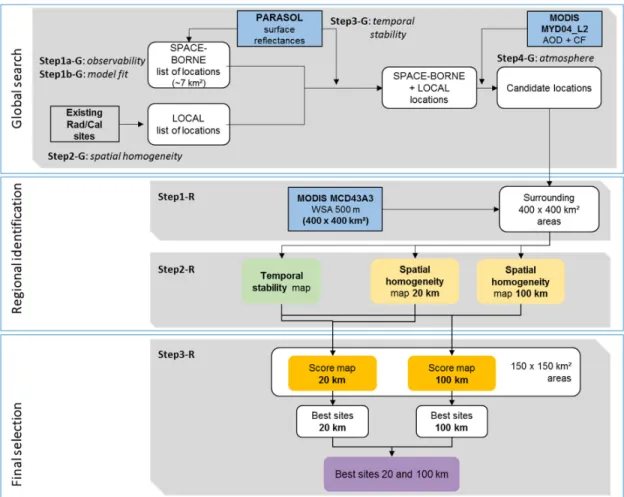
The procedure to identify possible PIC sites is depicted in Figure 1. First, a search at the global scale was performed with the aim to identify candidate areas of about 400 × 400 km² for which a refined characterization of the surface properties was performed at a second stage. The first stage relied on coarse scale PARASOL observations to infer a first estimate of a few characteristics (observability, reproducibility of the directional signatures, temporal stability of the surface reflectance over one year) of land desert pixels at coarse spatial resolution, and on MODIS MYD04_L2 AOD and cloud fraction products to characterize mean atmosphere properties (and hence the observability of the surface from space). The second stage relied on MODIS WCD43A3 WSA data to characterize the temporal stability of the surface at 500 m and the spatial homogeneity of selected areas at 20 × 20 km² and 100 × 100 km². The final stage consisted of combining these metrics in order to identify the most relevant locations. The analysis, both for PARASOL and MCD43A3, relies mostly on surface reflectance at 670 and 865 nm.

Figure 1. Flowchart of the selection steps used for identifying the most relevant sand desert PIC sites

for 20 km and 100 km scale applications.

3.1.1. Metrics

The spatial homogeneity of the areas of interest is defined on a pixel per pixel basis by measuring

the variability (standard deviation) σ of the surface reflectance _ within its neighborhood, as in

Cosnefroy [1]. The spatial homogeneity (in %) of a given pixel is measured by:

𝑆𝐻𝑜𝑚_(𝑋𝑘𝑚) = 100 × 𝜎(𝜌− 𝜌, )

𝜌_, (1)

with 𝜌, the mean reflectance in spectral band  over its surrounding neighborhood within X

km distance: 20 km (±40 pixels from either side of the considered pixel using WSA products at 500 m) or 100 km (±200 pixels).

The temporal stability (in %) characterizes the variability of a pixel reflectance relative to the averaged reflectance (_,) over the whole of the time series:

𝑇𝑉𝑎𝑟_ = 100 ×𝜎







The final site identification was based on scores combining temporal stability and spatial homogeneity maps derived from MODIS MCD43A3 products. Given that the spatial homogeneity maps correspond to spatially smoothed metrics, we also defined a spatially smoothed temporal stability as:

𝑇𝑉𝑎𝑟_(𝑋𝑘𝑚) =1

𝑛 𝑇𝑉𝑎𝑟 (3)

With n the number of pixels within the sliding window considered over 20 km / 100 km scales. Finally, three scores were defined to identify the best locations at 20 km, at 100 km, and at the two resolutions:

𝑆𝑐𝑜𝑟𝑒(



𝑆𝑐𝑜𝑟𝑒(



𝑆𝑐𝑜𝑟𝑒(







The weighting coefficient α was assigned a value of 2 so as to give more importance to the temporal stability criterion which is a site property of higher priority than spatial uniformity (the impact of the value of α on the site identification is discussed in Section 6.3). Note that in the following, we did not used strong threshold values on these metrics to screen the less desirable locations; rather, the identification procedure aimed at seeking for locations that provides optimal (i.e., minimal) values of these metrics, based on their distribution.

3.1.2. Global Scale Iteration

A four-step selection procedure was applied to establish a first list of relevant areas at the global scale. It relied mostly on space-borne PARASOL data but also considered existing calibration sites (including the 20 Cosnefroy PICS).

Monthly PARASOL data over year 2008 were used to establish a first list of relevant coarse resolution desert pixels (~7 km) from a global search. We sought for potential calibration pixels distributed all over the globe verifying several selection criteria: (1) the pixels should be thematically homogeneous desert areas, (2) the surrounding areas should be as flat as possible to minimize directional effects associated with topography variations as well as environmental effects, (3) their optical properties should be stable in time, and (4) their spectro-directional signatures should be reproducible using semi-empirical BRDF models. Regarding the latter criterion, poor fit could indeed be explained by contaminations by atmospheric effects (unresolved aerosols for instance) or changes in the surface condition within a month (effect of soil moisture on the reflectance levels after precipitations, greening/senescence of vegetation, etc.) which are features to be avoided for PIC sites. PARASOL data were processed only for pixels (~7 km) corresponding to (i) 100% of the IGBP "Barren or sparsely vegetated" class at 1 km, and to (ii) “flat” areas. The “flatness” of any pixel was here characterized as the standard deviation of the topography over its 60 × 60 km² surrounding area based on GTOPO30 data; pixels with a standard deviation exceeding 50 m were discarded.

• Step1-G (identification of candidate locations from PARASOL): The processing of PARASOL

observations is performed in two successive steps:

- Step1a-G (observability): A first screening was performed by selecting only the pixels which are

seen more than four days a month, and with more than 5 months respecting that criterion. Indeed, the number of observations is an indicator of the pixel observability: low observation numbers are likely due to cloud coverage or atmospheric effects (aerosols) precluding their monitoring.

- Step1b-G (reproducibility of the directional signatures): First, the Ross-Li-HS model was inverted

that the surface optical properties remain stable within a month, which is the main criterion for sand PICS. The Ross-Li-HS model was selected a priori based on the results of Maignan [38], showing it provides the best fitting capacities over various land surfaces (vegetation and soil) among several semi-empirical kernel driven models. From the optimized model, we derived the monthly normalized reflectances in the red and near infrared bands, which are used to quantify the temporal stability of the surface properties over one typical year. We attributed to each pixel a score that quantifies the overall quality of fit (characterized by the Root Mean Square Difference – RMSD) weighted by the number of measurements available per month. Then, filtering based on the (i) quality of fit and (ii) temporal stability of the inferred normalized reflectances was performed to retain the locations providing the best compromise between these quality scores. This filtering was performed country by country in order to identify candidate locations distributed world-wide (a global search would have otherwise favored too many sites over Sahara or Saudi Arabia): For each country, we kept a maximum of 20 locations with fitting scores falling in the upper 15th percentile of their associated distribution and with temporal stability at 670 and 865 nm within their 30th _percentile.

• Step2-G (existing Rad/Cal sites): the list of candidate locations was completed by already existing

calibration sites as listed in Berthelot [25]. For the site coordinates available, we performed a simple appraisal of their spatial homogeneity at a 20 km scale by a visual inspection of corresponding Google Maps images, and we discarded the ones that were obviously too heterogeneous. We also discarded sites where less than nine months were monitored by PARASOL for at least four days, as lower numbers indicate low site observability (note that the observability criterion was deliberately relaxed as compared to Step1-Ga: five months with acquisitions at least on four days). Monthly PARASOL observations over 2008 were then retrieved for the sites identified in order to apply the next processing step.

• Step3-G (temporal stability): for the locations inferred from Step1-G and Step2-G, we retained

those exhibiting the highest temporal stability of the normalized reflectances inferred from the inversion of the RossLi-HS model over monthly PARASOL data. The screening was performed on the averaged value of TVar (Equation 2) over all channels but the one at 490 nm (which usually provides a lower sensor signal-to-noise than the others due to both higher atmospheric scattering and lower reflectance levels). Only the locations with an averaged TVar value below the 25th percentile of the distribution over all candidate locations were retained.

• Step4-G (atmosphere properties): A final screening was performed depending on the atmosphere

characteristics of the selected sites. For each location the median values and standard deviation of the Deep Blue AOD at 550 nm and of the cloud fraction were estimated based on the MYD04_L2 products. The locations whose AOD standard deviation and median values were above the 85th percentile of the corresponding distribution were removed. In addition, locations with median cloud coverage value above the 85th percentile were also removed together with those with more than 50% of the observations with a cloud fraction above that value.

• Step1-R: We identified ~400 × 400 km² areas encompassing the locations selected in the previous step, and retrieved the corresponding MODIS MCD43A3-WSA products described earlier. The MODIS products were re-projected into the World Geodetic System 84 to facilitate the geo-referencing across sites, using an increment in latitude and longitude that was the closest possible to the original resolution of the products (0.00462° which is about equivalent to 500 m). The re-projection was performed using the Gdal library in Python.

• Step2-R: For each area, the temporal stability (Equation 2 and Equation 3) was then quantified and also for the spatial homogeneity at 20 km and 100 km (Equation 1) of each pixel. In order to reduce the computational time, we further limited the processing to 150 × 150 km² areas (~300× 300 pixels at 500 m resolution) surrounding the locations exhibiting the highest spatial uniformity at 20 km (estimated from a visual appraisal of the maps generated, see Section 4.2).

• Step3-R: The scores combining temporal stability and spatial uniformity were then determined over these 150 × 150 km² areas (Equation 5 to 7). Finally, the “optimal” locations were identified as those providing the best scores at 20 km, 100 km, and for both resolutions. The final location is determined, over the 30 pixels that minimize a given score, as the barycenter of the highest point density.

We focused the analysis on the metrics estimated at 865 nm.

3.2. Characterization of Surface Reflectance Anisotropy

3.2.1. BRDF Model Inversion

The BRDF models were fitted against the monthly PARASOL observations described earlier. We applied a different optimization procedure depending on the model linearity. For linear models, the weighting parameters K of each kernel were optimized so as to minimize the RMSD between measurements and model outputs using a simple matrix inversion

𝐊 = (𝐅 𝐅) 𝐅 𝐘, (7) where Y is a 1xN matrix representing the column vectors of the N observations and F an mxN matrix

representing corresponding N simulations for each of the m kernel. For non-linear models, the optimization was performed using the curve_fit non-linear least square function of the Scipy library for Python. In order to minimize the impact of the set of initial parameter guesses on the solution, 10 optimizations were run with different initial guesses. The retained final solution was the one leading to the lower RMS difference between model and data. In case of convergence issues, we did not consider the corresponding observation data in the analysis.

The magnitude of the directional variations of the surface reflectance was quantified for each of the final PIC sites, in each PARASOL band. To do so, one BRDF model was fitted over the whole of PARASOL available over the year 2008 (for each band). In order to remove observations possibly impacted by remaining contamination by atmospheric effects, only 80% of the observations providing the best agreement with the model were kept. The model was then inverted again on this subset in order to determine a "yearly model" (with associated parameters) for each site.

From these retrieved BRDF model parameters, a typical directional reflectance signature was then computed for a sun zenith angle equal to that of the average over all available observations. The site anisotropy is quantified as the relative variability of the reflectance 𝜌 in the principal plane, for

view zenith angles (VZA) less than 60°, and excluding those observations that are less than 10° from backscatter as they may be impacted by the hot spot effect.

The magnitude of the directional effects in each waveband  is then expressed (in %) as a

function of the averaged reflectance 𝜌 over all considered viewing geometries as:

𝐵𝑅𝐷𝐹𝑚𝑎𝑔𝑛𝑖𝑡𝑢𝑑𝑒(



𝜌_ (8)

4. Results of the Identification of PIC Sites

4.1. Global Scale Search

About 74 000 PARASOL pixels were identified after Step1a-G, spreading over 40 countries worldwide. The fitting scores and temporal stabilities at 670 nm per country are shown in Figure 2 as boxplots characterizing the distribution of the two metrics. Pixels located in China, Kazakhstan, Mongolia, Turkmenistan, United States and Uzbekistan exhibit higher temporal variability (i.e., lower temporal stability). These countries are also associated with the lowest fitting scores. The filtering approach at Step1b-G based on the joint removal of pixels (i) with directional signatures not well reproduced by the Ross-Li-HS BRDF model and (ii) low temporal stability of the retrieved normalized reflectances (in the red and near infrared bands) led to a significant decrease of the number of candidate pixels to only 473.

Figure 2. For about 74 000 pixels spanning 40 countries, boxplots by country: (Top) the score of fit of

the monthly PARASOL directional observations by the Ross-Li-HS BRDF model at 670 nm, and (Bottom) the temporal variability over one year (2008) of the normalized reflectances at 670 nm. The boxplot extends from the 25th and 75th percentile of the value distribution, with a line at the median. The number of pixels considered for each country is provided in parentheses.

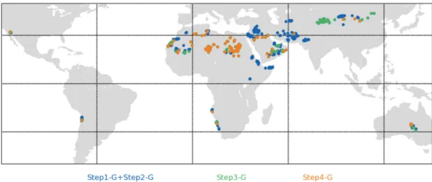
The list of pixels inferred from PARASOL was completed by 78 existing calibration sites

(Step2-G) [25], including the twenty Cosnefroy sites. They are located in Algeria (6 sites), Arabia (9),

Australia (5), China (25), Egypt (3), Iraq (2), Libya (8), Mali (1), Mauritania (3), Namibia (3), Niger (4), Sudan (5), Tunisia (1), USA (2), and Yemen (1). Figure 3 illustrates how candidate locations are screened along the successive screening steps. The screening of the locations based on the temporal stability performed at Step3-G reduced the number of candidate locations to 178. The discarded locations were mainly located in Middle East, Central Asia, China and in the Horn of Africa, as depicted by the blue dots in Figure 3. The threshold value of the 25th percentile of the TVar values averaged over all PARASOL bands but 490 nm was 0.013. The screening performed at Step4-G on the AOD and cloud fraction variables removed 63 locations (green dots in in Figure 3), most of them being located in China, as well as Mauritania and Arabia. Noteworthy, the Cosnefroy PICS Mali1 and Arabia2 were among the discarded locations, due to AOD loads (median values of 0.39 and 0.41) exceeding the estimated threshold on the median AOD values (0.38). The threshold values for selection related to AOD standard deviation and median CF values were 0.36 and 0.09, respectively. The screening resulted in a shortened list of 115 candidate locations (orange dots in Figure 3).

Figure 3. Candidate locations inferred from the global scale processing along the successive screening

steps: Step1-G+Step2-G (blue), Step3-G (green) and Step4-G (orange).

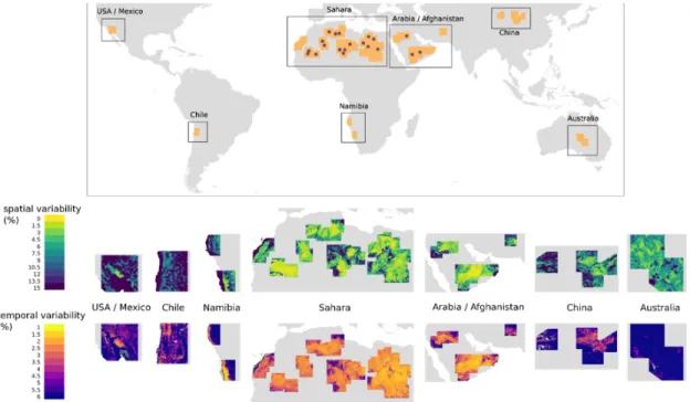
4.2. Regional Scale Search

We then identified 71 regions of 400 × 400 km² encompassing the 115 locations identified in the previous step and retrieved the corresponding MODIS WCD43A3-WSA data (Step1-R). The temporal stability (Equation 2) and spatial homogeneity (Equation 1) were computed at 20 km resolution for each component pixel. The resulting maps are presented in Figure 4 (from WSA data at 865 nm), grouped over large regions. The temporal stability and spatial homogeneity maps usually present similar spatial patterns. The regions selected in Sahara and Arabian Peninsula are those exhibiting the highest spatial uniformity (spatial variability at 20 km below 3% typically) and temporal stability (temporal variability below 2%) over large spatial extents. Similar spatial uniformity values may be found in the USA (region overlapping South California, Arizona and Mexico), Chile, northern Namibia and western China, but they spread over much smaller areas. This also holds for the temporal stability. While the selected regions in Australia present relatively high spatial uniformity over large spatial scales (with variability at 20 km below 6% typically), their optical properties are more unstable over time (temporal variability at 865 nm above 8%). A threshold value of temporal

stability set at 3% thus excludes all regions not located in the Sahara and Arabian peninsula, but one located in the southern part of Namibia where a narrow band parallel to the coast exhibits about as high a spatial uniformity and temporal stability as the Saharan and Arabian regions. Note that the map of the spatial uniformity at 100 km is even more restrictive in terms of candidate areas (results not shown). Indeed, only a few regions in south east Arabia, Mauritania, Algeria, Libya and Niger, present large a spatial extent with spatial variability below 3%, the lowest values being found for Arabia and Mauritania at 100 km.

Figure 4. Maps of the a) spatial uniformity at 20 km and b) temporal stability, inferred from MCD43A3

– WSA products at 865 nm and zoomed over large regions of interest . The locations of the 20 PIC sites identified by Cosnefroy [1] are shown as dots on the global map at the top.

For the calculation of the scores (at 20 km and 100 km) at Step2-R, we focused on 60 areas of 150 × 150 km² corresponding to those exhibiting the highest spatial uniformity and temporal stability over large surfaces. They are thus located in Namibia, Sahara and Arabian Peninsula. For 20 of these areas, their center corresponds to one of the 20 Cosnefroy’s PIC sites.

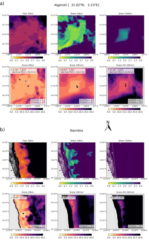
The identification of the optimal locations, i.e., those providing the best scores at 20 km and 100 km, are illustrated for one Cosnefroy’s PIC site (Algeria5) and for Namibia in Figure 5. The figure shows the maps of temporal stability, spatial homogeneities and scores over 150 × 150 km² areas. These two regions present pixels with similar high spatial homogeneity at 20 km (below 2%) but are distributed over larger surfaces in the case of Algeria. The central part of the Algeria region (around the Algeria5 PICS) also presents contiguous pixels with high spatial homogeneity at 100 km, below 3%. By contrast, the region in Namibia is more heterogeneous and does not offer any pixel with a spatial variability at 100 km below 4%. On another hand, the coastal band in Namibia displays a higher temporal stability (relative variation between 1–2%) than the Algerian region (between 2–3%). For Algeria5, there are several distant pixels, among the 30 best ones selected over the whole region, that have low score values at 20 km (corresponding to “ideal” locations with low temporal variability and low spatial heterogeneity). The barycenter is located 78 km at the north west of the original Algeria5 site. The difference in terms of the score value is low (0.05). For the score at 100 km and the score combining the two resolutions, the optimal locations are even closer to the original PICS (less than 15 km away from it). In particular, at 100 km, the performances of the pixels surrounding Algeria5 cannot be distinguished. The location identified in Namibia (25°S; 15.25°E) provides a better

(lower) score at 20 km than the optimal location near Algeria5. It is explained by its higher temporal stability whereas its spatial homogeneity is slightly lower than for the Algerian site.

Figure 5. For a) the region surrounding Algeria5 PIC site and b) the identified region in Namibia,

maps of the temporal stability at 20 km (TVar) and spatial homogeneity (SHom) at 20 and 100 km (top), and scores (in %) at 20, 100, and 20+100 km (bottom), inferred from 865 nm WSA data. For each score map, the best location is shown as a star, and its (lat, lon) coordinates and score value are provided. For Algeria5 (shown as the square at the center of the score maps), are also indicated the corresponding score and the distance of the “best” location. The grey dots correspond to the 30 coordinates with the highest scores.

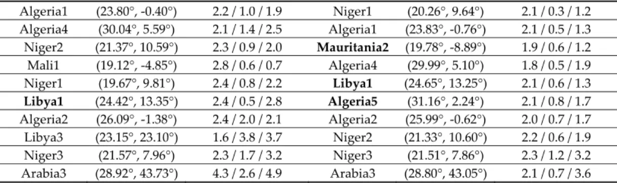
4.3. Performances of the 20 Cosnefroy PICS

The performances, in terms of temporal stability and spatial homogeneity, of the 20 PICS defined by Cosnefroy [1] are compared to those of the optimal locations in their vicinity (within a 150 km distance) relative to the score combining the two resolutions considered (𝑆𝑐𝑜𝑟𝑒(865𝑛𝑚|20 + 100𝑘𝑚)) (Table1 and Table 2). The sites that provide the best performances with respect to that score are Arabia2, Sudan1, Arabia1 and Egypt1. Their ranking is similar considering either the original or the optimal locations. Their high temporal stability (at 20 km) combined to their high spatial homogeneity at the two resolutions (below the 25th percentile of the distribution of each metrics) explain their high ranking. Five of the six IVOS sites (Algeria3, Mauritania1, Libya4, Mauritania2, and Algeria5) have temporal stability and spatial homogeneity values mostly below the median values of the corresponding distributions over all twenty sites. Although Libya1 exhibits a high spatial homogeneity at 20 km (value below the 25th percentile), it has poorer temporal stability and spatial uniformity at 100 km (above the 75th percentile of the respective distributions). The optimal locations in their vicinity provide only marginal improvements of these metrics: the improvement in temporal stability is only of 8.0% in average (ranging from 1.9% for Libya4 to 12.6% for Mauritania1); it is an average of 9.1% for the spatial homogeneity at 20 km (from 4.3% for Libya4 to 14.1% for Mauritania1), and of 8.9% for the spatial homogeneity at 100 km (from 0.5% for Algeria5 to 19.3% for Libya1). Over all sites, the improvements are slightly higher: 12.5% on average for TVar(20km), 18.9% and 9.8% for SHom(20km) and SHom(100km), respectively (using WSA at 865 nm). The lowest improvements are found for Niger3 (4% for SHom(100km), while no change is seen in the temporal stability at 20km) and Libya4 (4.3% for SHom(100km)). For all metrics considered, the highest improvements are obtained for Arabia3 (51.4% for the temporal stability at 20 km, and 56.6% and 30.7% for the spatial homogeneity at 20 km and 100 km). It is noteworthy that this site provides rather poor performances for all metrics. As seen in Figure 4, it is the site located in the northern part of Saudi Arabia which falls into a transition zone with changing and high temporal variabilities.

Table 1. For the original 20 PICS identified by Cosnefroy [1] and the "optimal" locations in their

vicinity providing the best scores at 20+100 km (at 865 nm), values of the 25th/ 50th/ 75th percentiles of the distribution of the following metrics: temporal stability at 20 km (TVar(20km)), spatial homogeneity at 20 km (SHom(20km)) and at 100 km (SHom(100 km)).

TVar(20km) (%) SHom(20km) (%) SHom(100km) (%)

Original locations 2.1 / 2.2 / 2.3 0.6 / 0.8 / 1.2 1.5 / 1.9 / 2.3

Optimal locations 1.8 / 2.0 / 2.1 0.4 / 0.5 / 0.7 1.1 / 1.3 / 1.8

Table 2. Performance metrics for the original 20 PICS identified by Cosnefroy [1] and the

corresponding "optimal" locations in their vicinity (providing the best scores at 20 + 100 km): temporal stability at 20 km (TVar(20km)), the spatial homogeneity at 20 km and at 100 km (SHom(20km) and SHom(100km)). The metrics are calculated from WSA at 865 nm. The sites are sorted based on the score values at 20 + 100 km (𝑆𝑐𝑜𝑟𝑒(865𝑛𝑚|20 + 100𝑘𝑚)). The six sites in bold are the IVOS sites.

Original PICS locations Optimal locations

name (lat, lon)

TVar(20km) / SHom(20km) / SHom(100km) (%)

name (lat, lon)

TVar(20km) / SHom(20km) / SHom(100km) (%) Arabia2 (20.13°, 50.96°) 1.6 / 0.3 / 1.1 Arabia2 (20.19°, 51.63°) 1.4 / 0.2 / 0.4 Sudan1 (21.74°, 28.22°) 1.6 / 0.8 / 1.6 Sudan1 (22.11°, 28.11°) 1.5 / 0.5 / 1.2 Arabia1 (18.88°, 46.76°) 1.7 / 1.1 / 1.8 Arabia1 (19.80°, 47.07°) 1.4 / 0.4 / 1.4 Egypt1 (27.12°, 26.10°) 2.2 / 0.6 / 1.1 Egypt1 (26.61°, 26.22°) 1.9 / 0.5 / 0.9 Libya2 (25.05°, 20.48°) 2.2 / 0.6 / 1.3 Libya3 (23.22°, 23.23°) 1.4 / 0.4 / 3.1 Algeria3 (30.32°, 7.66°) 2.1 / 0.9 / 1.8 Libya2 (25.08°, 20.77°) 2.0 / 0.4 / 1.1 Mauritania1 (19.40°, -9.30°) 2.2 / 0.8 / 1.3 Algeria3 (30.63°, 7.83°) 2.0 / 0.7 / 1.4 Libya4 (28.55°, 23.39°) 2.1 / 0.7 / 1.7 Mauritania1 (19.51°, -8.57°) 1.9 / 0.6 / 0.9 Mauritania2 (20.85°, -8.78°) 2.2 / 0.6 / 2.1 Mali1 (19.14°, -5.77°) 2.2 / 0.3 / 0.6 Algeria5 (31.02°, 2.23°) 2.2 / 0.9 / 1.8 Libya4 (28.67°, 23.42°) 2.1 / 0.6 / 1.0

Algeria1 (23.80°, -0.40°) 2.2 / 1.0 / 1.9 Niger1 (20.26°, 9.64°) 2.1 / 0.3 / 1.2 Algeria4 (30.04°, 5.59°) 2.1 / 1.4 / 2.5 Algeria1 (23.83°, -0.76°) 2.1 / 0.5 / 1.3 Niger2 (21.37°, 10.59°) 2.3 / 0.9 / 2.0 Mauritania2 (19.78°, -8.89°) 1.9 / 0.6 / 1.2 Mali1 (19.12°, -4.85°) 2.8 / 0.6 / 0.7 Algeria4 (29.99°, 5.10°) 1.8 / 0.5 / 1.9 Niger1 (19.67°, 9.81°) 2.4 / 0.8 / 2.2 Libya1 (24.65°, 13.25°) 2.1 / 0.6 / 1.3 Libya1 (24.42°, 13.35°) 2.4 / 0.5 / 2.8 Algeria5 (31.16°, 2.24°) 2.1 / 0.8 / 1.7 Algeria2 (26.09°, -1.38°) 2.4 / 2.0 / 2.1 Algeria2 (25.99°, -0.62°) 2.0 / 0.7 / 1.7 Libya3 (23.15°, 23.10°) 1.6 / 3.8 / 3.7 Niger2 (21.33°, 10.60°) 2.2 / 0.6 / 1.9 Niger3 (21.57°, 7.96°) 2.3 / 1.7 / 3.2 Niger3 (21.51°, 7.86°) 2.3 / 1.2 / 3.2 Arabia3 (28.92°, 43.73°) 4.3 / 2.6 / 4.9 Arabia3 (28.80°, 43.05°) 2.1 / 0.7 / 3.6

4.4. Identification of New Sites of Interest

The metrics determined above for the original 20 PICS were used as benchmarks for assessing the relevance of additional sites. We identified four sites based on their score values (at 20+100 km for all sites except Namibia where only the 20 km resolution is considered) and that are not in the “close” vicinity (see Section 4.3) of the 20 Cosnefroy sites. The values of their temporal stability and spatial homogeneity metrics at 865 nm are provided in Table 3. They generally provide performances

below the 50th _{percentile estimated from the original Cosnefroy PIC sites, and below the 75th}

percentile for their updated locations (cf. Table 1). The site in Namibia shows poor performances at 100 km, as already highlighted in Figure 5-b. It is located about 160 km south-east of Gobabeb (S23.55°, E15.03°). The site in Algeria remains close to Algeria3 (about 170 km away, in a north-easterly direction). The site in Arabia is located about 280 km west of Arabia3. The site in Sudan is 570 km away from Sudan1, towards the south west.

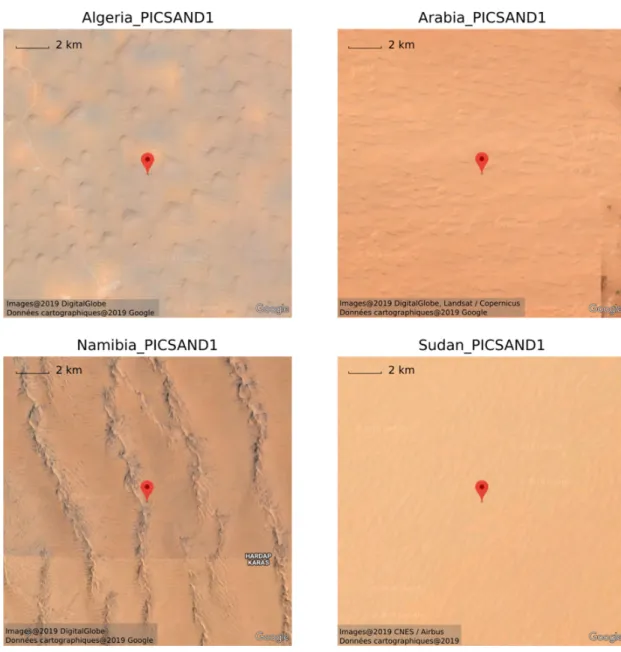
The landscape heterogeneity around the sites can be appraised qualitatively on Google Map images of 15 × 15 km² areas (Figure 6). Some artefacts are visible on some images, for instance, the image composed of different satellite overpass leading to strong latitudinal discontinuities for Namibia_PICSAND1 or clouds casting shadows at Arabia_PICSAND1. At the zoom level considered, Namibia_PICSAND1 appears the most heterogeneous site with North-South orientated dune structures.

Table 3. Auxiliary PIC sites providing high joint performances at 20 km and 100 km: name,

coordinates and values of the temporal stability at 20 km (TVar(20km)), the spatial homogeneity at 20 km and at 100 km (SHom(20km) and SHom(100km)).

Name (llat, lon)

TVar(20km) / SHom(20km) / SHom(100km) (%) Algeria_PICSAND1 (31.70°, 8.35°) 2.1 / 0.6 / 1.1 Arabia_PICSAND1 (29.26°, 40.91°) 1.9 / 0.5 / 2.2 Namibia_PICSAND1 (-25.00°, 15.25°) 1.2 / 0.9 / 5.3 Sudan_PICSAND1 (17.26°, 25.53°) 1.7 / 0.7 / 1.7

Figure 6. Google Map images of about 15 × 15 km² around the four sites identified. The screenshots were acquired on February 2019.

5. PICS Properties

The surface and atmospheric properties are characterized below for the six IVOS sites that are the most commonly used (Algeria3, Algeria5, Libya1, Libya4, Mauritania1, Mauritania2) and for the four candidate sites identified above.

5.1. Characterization of Surface Spectro-Directional Reflectance

5.1.1. Fitting Performance of the BRDF Models

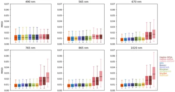
Before quantifying the magnitude of the directional effects of the ten sites considered, the fitting performances of the BRDF models were evaluated against monthly PARASOL data in each band. Observations around the hot spot direction (phase angle lower than 10°) were removed for the model optimization. The residual RMSD between the calibrated model and the observations averaged over all sites are presented as boxplots for each waveband in Figure 7.

The Snyder and RPV models generally provide the best fitting performances in all wavebands for all sites. The fitting performances of Ross-Li-HS, followed by Ross-Li/Roujean/Roujean-HS are

slightly lower than those of Snyder and RPV: the median RMSD values obtained with Ross-Li-HS are between 5% to 12% higher than Snyder depending of the waveband, between 6%–12% for RossLi, and between 5 and 16% for the two versions of the Roujean model. The “superiority” of the Snyder and RPV models over the other models is smoothed out in the blue band and in the near infrared at all sites but Namibia_PICSAND1, where Snyder and RPV show higher fitting performances in all PARASOL bands.

Although the fitting capacities of the Walthall model may be slightly superior to these semi-empirical kernel-driven models in the blue and green bands, its performances are lower in the red and near infrared bands. The three versions of the Hapke model provide the lowest fitting performances, with RMSD values increasing with wavelength. This is likely attributed to a higher non-linearity of the model as compared to the other models, associated with a higher number of parameters to optimize. Note that in several cases, the curve_fit optimization routine (with its default parameterization) reported convergence issues with the Hapke and Snyder models.

Noticeably, the residual RMSD in the blue is higher than the RMSD in the near infrared bands. This is attributed to unresolved atmospheric effects (aerosols in particular) that the models are not designed to capture. This higher noise in the measurements also levels out the fitting performances between models.

Figure 7. For each PARASOL band, boxplots of RMSD of fit for the BRDF models relative to the

monthly data averaged over all 10 selected PICS. The median RMSD values are shown as black horizontal bars. In each waveband, the models are sorted by increasing order of the median RMSD values.

5.1.2. Magnitude of the Directional Effect

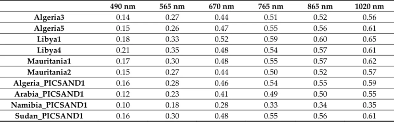
The quantification of the directional effect magnitude was performed with the Ross-Li-HS model because its linear form makes it easy to use. Figure 8 shows the variation of the relative magnitude of the directional effects relative to the mean reflectance for the 10 studied PICS. All of the selected sites exhibit reflectance variations due to surface anisotropy that is below 10%. The directional effects decrease with increasing reflectance levels (typically from the visible to the near-infrared). The lowest BRDF effects, in all PARASOL bands, are found for the two sites in Mauritania and for Sudan_PICSAND1. The site in Namibia exhibits, at the same time, higher surface anisotropy and lower reflectance levels (Table 4). In particular, its mean normalized reflectance at 670 nm is 0.28 and 0.34 at 865 nm, when the lowest values over the other sites are, respectively, of 0.41 and 0.50 (both for Arabia_PICSAND1). Note that the value of the normalized reflectances provided in Table 4 for the IVOS sites slightly differ from other sources (for instance Lacherade [5]) depending on the data and method used to infer them.

We hence checked a posteriori the relevance of those sites for vicarious calibration: they exhibit low directional effects (about 5% on average, and below 10%) and high surface reflectances which are above the threshold of 0.3 [14, 15, 23] after 670 nm.

Figure 8. For the 10 selected PIC sites, variation of the relative magnitude of the directional effects as

a function of the averaged reflectance over yearly data in each PARASOL band.

Table 4. Values of the normalized reflectance in PARASOL bands at nadir viewing and for a sun

zenith angle at 30°, estimated with the Ross-Li-HS model fitted over yearly PARASOL observations.

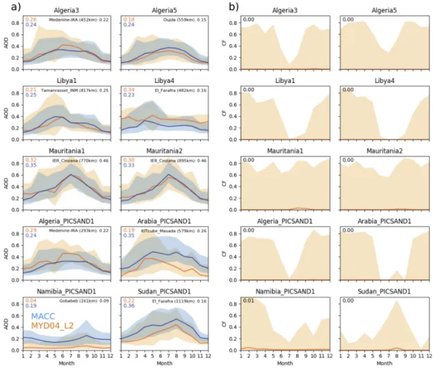
490 nm 565 nm 670 nm 765 nm 865 nm 1020 nm Algeria3 0.14 0.27 0.44 0.51 0.52 0.56 Algeria5 0.15 0.26 0.47 0.55 0.56 0.61 Libya1 0.18 0.33 0.52 0.59 0.60 0.65 Libya4 0.21 0.35 0.48 0.54 0.57 0.61 Mauritania1 0.17 0.30 0.48 0.55 0.57 0.62 Mauritania2 0.15 0.27 0.44 0.50 0.52 0.57 Algeria_PICSAND1 0.16 0.28 0.46 0.54 0.55 0.59 Arabia_PICSAND1 0.12 0.23 0.41 0.49 0.50 0.55 Namibia_PICSAND1 0.10 0.18 0.28 0.33 0.34 0.35 Sudan_PICSAND1 0.16 0.30 0.48 0.55 0.56 0.61 5.2. Atmosphere Characterization

The monthly climatologies (monthly medians) of aerosol optical depth (AOD) and cloud fraction (CF) derived from MODIS MYD04_L2 and MACC products are shown in Figure 9. For MYD04_L2 (~0.1° resolution), we considered all observations within a 0.2° lat/lon distance from the considered PICS; For the MACC data (1° resolution), we considered the grid cells containing the PICS. The “typical” monthly values are determined as the median of all data within each month. The AOD climatologies derived from the two datasets agree generally well in terms of median AOD and seasonality, the maximum AOD values being reached in spring or summer depending on the site. Discrepancies are, however, noticeable for Libya4 and for the four sites identified in this study: AOD

estimates inferred from MYD04_L2 are higher than the MACC estimates at Libya4 and Algeria_PICSAND1 while the opposite is observed at the three other sites. MYD04_L2-derived climatology also produces weaker amplitudes at Libya4 and Namibia_PICSAND1 than MACC. For all sites considered, the median AOD along a typical year is below 0.35. The Mauritanian sites have the highest AOD (from the two datasets). The other sites have median AOD values typically about 0.25-0.3, with the noticeable exception of Namibia_PICSAND1 which exhibit the lowest AOD (below 0.2, depending on the dataset). High AOD values (above 0.6) can be reached in spring or summer. Values above 1 in the two products possibly indicate occurrence of sand storms.

The AOD composition derived from the MACC products indicates that dust is the dominant aerosol type for all sites. The dust fractions are: 49% for Namibia_PICSAND1, 52% for Libya4, 55% for Algeria_PICSAND1, 59% for Algeria5, 62% for Algeria3, 63% for Arabia_PICSAND1, 70% for Sudan_PICSAND1 and Libya1, 74% for Mauritania2 and 76% for Mauritania1. The second contributor to AOD is sulfate: it is on the order of 15% for the two sites in Mauritania and Namibia_PICSAND1, 20% for Libya1 and Sudan_PICSAND1, 25% for Algeria3 and Algeria5, and 30% for Algeria_PICSAND1, Arabia_PICSAND1 and Libya4. The contributions of black carbon and organic matter are below 5%, except for Namibia_PICSAND1 (8% and 18%, respectively). The contribution of sea salt is below 10% for all sites, with some site variability. The highest values are found for Namibia_PICSAND1 (9%), and Algeria5 and Algeria_PICSAND1 (both about 8%). The median values of the Angström coefficient inferred from MYD04_L2 are 0 for all sites but two, indicating rather coarse aerosols. The exceptions are Arabia_PICSAND1 and Namibia_PICSAND1 with median value of 0.91 and 0.58, respectively, indicating a strong contribution by non-desert aerosol types. For the latter site, located about 15 km from the Namibian shores, the main source of uncertainty for the correction of aerosols is likely related to the type of aerosols. Indeed, Namibia_PICSAND1 is strongly affected by aerosols generated by fires within the African continent during the dry season that starts in May-June, as depicted by the contribution of black carbon and organic matter aerosol types. There are no such fires in the vicinity of the Arabia_PICSAND1 site, but anthropogenic contribution from Europe and the Indian subcontinent does contribute to the fine aerosol mode.

The monthly median cloud fraction (CF) is usually close to 0 and the monthly mean (not shown) shows a low seasonality. This guarantees that the sites are observable most of the year. CF can, however, reach high values (above 0.6) which may preclude the monitoring of a particular site. The

seasonality of the 90th _{CF percentile informs about the optimal time window for the site observations:}

for seven sites out of 10, the lowest CF values are obtained in July–August. Note that the opposite is seen for Sudan_PICSAND1 where the highest CF values are seen in summer. However, although these periods have the lowest cloud coverage, they are also often associated with high aerosol loads. The seasonality of CF for Namibia_PICSAND1 is more pronounced than for the other sites, and shows higher values from January to April; these months should therefore be avoided for in-flight calibration.

Figure 9. For the 10 selected PIC sites, monthly climatologies (median values) of (a) AOD (derived

from MYD04_L2 - orange - and MACC - blue - products), and (b) CF (from MYD04_L2). For each are displayed the median values plus-minus the 10th _{and 90}th _{percentile of the value distribution for each}

month. The top-left numbers correspond to the median values over a typical year. For AOD, the median value retrieved at the closest AERONET stations is indicated.

The seasonal cycle of the O3 atmospheric content (total column) has an amplitude that is typically

10% of the median value (Figure 10). Then, intra-month variability (standard deviation) is roughly of the same order. The sites show different seasonalities with higher values in winter for all sites but the two sites in Mauritania and Sudan_PICSAND1. For those, the higher values are reached in summer.

All sites also show a pronounced seasonality of the column-integrated H2O. The amplitude and the

intra-month variability are on the order of the median value. The maximum values are obtained in summer (July/August for sites in the Northern Hemisphere, January/December for the Namibia site).

Figure 10. Monthly climatologies (monthly medians) of the column integrated ozone (Dobson units)

and water vapour (cm) derived from MYD08_M3 for the 10 selected sites.

The mean number of days in a year with rainfall rate above 0 varies depending on the meteorological forcing used. In particular, CRU-NCEP provides the lowest values over all sites. The mean number of days in a year with rainfall, averaged over WSGWP3 and CERASAT outputs, varies between 7 (Libya1) and 35 (Algeria5) days. This highlights that the occurrence of rainfall is low for all sites. The sites in Libya in particular (11 days a year for Libya4) are less impacted by precipitation. For sites in Algeria, Libya, Arabia, the occurrence of rainfall is more important from November to February. For the Mauritanian sites and Sudan_PICSAND1, however, rainfall is rare in winter months and more frequent in August and September. For Namibia_PICSAND1, rainfall mostly occurs in January and February.

Surface pressure is a good proxy for the well mixed gases in the atmosphere (in particular CO2

and O2). Although the three meteorological forcings exhibit systematic differences in terms of surface

pressure magnitude which is due to differences in the mean altitude of the grid cells of the various products, we are mostly interested here in the typical surface pressure seasonality which is consistent between products. The amplitude of the variation of surface pressure is usually below 1% with respect to the average, with higher values in the winter months (January and December for sites in the Northern Hemisphere, July and August for Namibia_PICSAND1). Libya4 and Arabia_PICSAND1 show slightly higher variations (about 1.01% and 1.4%, respectively, depending on the forcing products).

6. Discussion

6.1 Remotely Sensed Products

In this work, we designed an approach to identify desert PICS distributed world-wide based on computational considerations, relying essentially on space-borne observations of their surface reflectance. The identification procedure and the determination of PICS optical properties relied on complementary informations from the PARASOL and MODIS instruments. The benefit of PARASOL is mostly related to its acquisition of multi-directional data, which provides a much more detailed description of the directional signature of the surface than MODIS does. MODIS, however, provides higher spatial and temporal monitoring over a longer time period. To evaluate the directional effects of the surface, we used one typical year (2008) of PARASOL observations. Given that (i) the study focuses on very stable targets, with negligible year-to-year variations and that (ii) the temporal variation of the directional signatures are even smaller than those of the overall reflectance, the choice of only one year of data for PARASOL has a negligible impact on the conclusions. As there is no overlapping period between PARASOL and MODIS observations used, we implicitly made the assumption that the desert targets do not vary significantly between 2008 and 2011.

Note that the reflective solar bands of the MODIS instrument are calibrated against an on-board solar diffuser and regular moon observations [49], and not on the desert sites analyzed here. The PARASOL satellite that carried the POLDER sensor was part of the Aqua Train and therefore shares its orbit characteristics: It was sun-synchronous with an equator crossing time around 1:30. The absolute calibration of PARASOL was based on the molecular scattering, whereas the inter-band calibration used glint viewing [50]. Bright stable targets, such as the desert sites analyzed here were used to monitor the multi-temporal evolution of the instrument calibration. Therefore, the absolute calibration of both PARASOL and MODIS is independent of the desert sites investigated here, and there is therefore no direct risk of circular reasoning that could impact our analysis.

6.2 Investigated Areas

The global search aimed at minimizing the amount of space-borne data to process in the second stage for characterizing spectral temporal stability and spatial uniformity at high (500 m) spatial resolution considering 20 km and 100 km scales. By the same logic, we limited our investigations to 400 × 400 km² and then 150 × 150 km² regions of interest after successive selections. In addition, we did not seek additional sites too close to already existing PICS. In order to distribute candidate space-borne pixels across the globe in Step1b-G, we applied a screening on a country basis by retaining a maximum of 20 locations per country. Although this approach is somewhat simplistic (and easy to implement), a more complex approach (for instance, selecting sites by X-degree by X-degree boxes) would have provided similar results given the goal of that preliminary processing step (identifying

400 × 400 km2 _{areas and determining their temporal stability and spatial uniformity).}

The selection procedure focused on spatially limited regions and did not rely on hard threshold values on temporal stability and spatial uniformity (at 20 km and 100 km scales) metrics to screen less appropriate areas, but rather aimed at identifying the “optimal” ones based on the distribution of those metrics over all regions investigated. In doing so, we may have excluded some regions also relevant for vicarious calibration scales. We did not quantify the impact of the size of the search regions (400 km and 150 km) on the final site selection, which was out of scope of the study. However, the possible excluded regions would most likely be in the Sahara and Arabian Peninsula, which would be fully redundant (same advantages and disadvantages) with the sites that were selected here.

Our selection procedure did not retain many existing Rad/Cal sites [25] that have a smaller spatial extent. The Simpson Desert region identified in Helder [16], although its spatial extent is about 100 km wide, was not retained because of lower temporal stabilities, as compared to the other regions. The spatial extent criterion was relaxed for the site in Namibia. The reason is that due to several ongoing initiatives for space-borne instrument calibration purposes based on collaboration between the Gobabeb Research Center and various European entities (e.g., European Space Agency / Centre National d'Etudes Spatiales (France) / National Physical Laboratory (UK)), the Namibian desert now offers relatively easy logistical access compare to other CEOS/WGCV/IVOS locations, making it an attractive alternative to establish new PICS and access them to characterize their sand properties.

Modern high spatial resolution sensors may be calibrated over much smaller dimension targets than the ones considered in this study. Relaxing the constraint on the spatial scale would then likely extend the number and the distribution over the globe of sand desert areas suitable for vicarious calibration.

6.3. Definition of Identification Metrics

The identification of PICS based on temporal stability and spatial uniformity metrics relied on WSA data at 865 nm. We obtained very similar results with the 670 nm products. In the definition of the score metrics, we chose to give two times more weight to temporal stability over spatial uniformity (𝛼 weighting coefficient set to 2). The reason is that temporal stability is the primary criterion that is required for PICS. The selected regions display spectral temporal stabilities over