HAL Id: hal-03209237
https://hal.archives-ouvertes.fr/hal-03209237
Submitted on 28 Apr 2021HAL is a multi-disciplinary open access archive for the deposit and dissemination of sci-entific research documents, whether they are pub-lished or not. The documents may come from teaching and research institutions in France or abroad, or from public or private research centers.
L’archive ouverte pluridisciplinaire HAL, est destinée au dépôt et à la diffusion de documents scientifiques de niveau recherche, publiés ou non, émanant des établissements d’enseignement et de recherche français ou étrangers, des laboratoires publics ou privés.
Satellite-Derived LAI over the High-Latitude Northern
Hemisphere. Part I: Uncoupled DGVMs
Guillermo Murray-Tortarolo, Alessandro Anav, Pierre Friedlingstein, Stephen
Sitch, Shilong Piao, Zaichun Zhu, Benjamin Poulter, Soenke Zaehle, Anders
Ahlström, Mark Lomas, et al.
To cite this version:
Guillermo Murray-Tortarolo, Alessandro Anav, Pierre Friedlingstein, Stephen Sitch, Shilong Piao, et al.. Evaluation of Land Surface Models in Reproducing Satellite-Derived LAI over the High-Latitude Northern Hemisphere. Part I: Uncoupled DGVMs. Remote Sensing, MDPI, 2013, 5 (10), pp.4819-4838. �10.3390/rs5104819�. �hal-03209237�
Remote Sensing
ISSN 2072-4292
www.mdpi.com/journal/remotesensing
Article
Evaluation of Land Surface Models in Reproducing
Satellite-Derived LAI over the High-Latitude Northern
Hemisphere. Part I: Uncoupled DGVMs
Guillermo Murray-Tortarolo 1,*, Alessandro Anav 1, Pierre Friedlingstein 1, Stephen Sitch 2, Shilong Piao 3, Zaichun Zhu 4, Benjamin Poulter 5, Sönke Zaehle 6, Anders Ahlström 7, Mark Lomas 8, Sam Levis 9, Nicholas Viovy 5 and Ning Zeng 10
1
College of Engineering, Mathematics & Physical Sciences, University of Exeter, Harrison Building, North Park Road, Exeter EX4 4QF, UK; E-Mails: A.Anav@exeter.ac.uk (A.A.);
P.Friedlingstein@exeter.ac.uk (P.F.)
2
College of Life and Environmental Sciences, University of Exeter, Amory Building, Rennes Drive, Exeter EX4 4RJ, UK; E-Mail: S.A.Sitch@exeter.ac.uk
3
Department of Ecology, Peking University, Beijing 100871, China; E-Mail: slpiao@pku.edu.cn
4
Department of Earth and Environment, Boston University, 675 Commonwealth Avenue, Boston, MA 02215, USA; E-Mail: zhu.zaichun@gmail.com
5
Laboratoire des Sciences du Climat et de l’Environnement, CEA CNRS UVSQ, Gif-sur-Yvette 91191, France; E-Mails: benjamin.poulter@lsce.ipsl.fr (B.P.); nicolas.viovy@lsce.ipsl.fr (N.V.)
6
Max Planck Institute for Biogeochemistry, P.O. Box 10 01 64, D-07701 Jena, Germany; E-Mail: szaehle@bgc-jena.mpg.de
7
Department of Physical Geography and Ecosystem Science, Lund University, Sölvegatan 12, SE-22362, Lund; E-Mail: anders.ahlstrom@nateko.lu.se
8
Department of Animal & Plant Sciences, University of Sheffield, Sheffield S10 2TN, UK; E-Mail: m.r.lomas@sheffield.ac.uk
9
National Center for Atmospheric Research, Boulder, CO80305, USA; E-Mail: slevis@ucar.edu
10
Department of Atmospheric and Oceanic Science, University of Maryland, College Park, MD 20740, USA; E-Mail: zeng@umd.edu
* Author to whom correspondence should be addressed; E-Mail: gnm202@ex.ac.uk;
Received: 15 August 2013; in revised form: 9 September 2013 / Accepted: 17 September 2013 / Published: 8 October 2013
Abstract: Leaf Area Index (LAI) represents the total surface area of leaves above a unit
area of ground and is a key variable in any vegetation model, as well as in climate models. New high resolution LAI satellite data is now available covering a period of several decades.
This provides a unique opportunity to validate LAI estimates from multiple vegetation models. The objective of this paper is to compare new, satellite-derived LAI measurements with modeled output for the Northern Hemisphere. We compare monthly LAI output from eight land surface models from the TRENDY compendium with satellite data from an Artificial Neural Network (ANN) from the latest version (third generation) of GIMMS AVHRR NDVI data over the period 1986–2005. Our results show that all the models overestimate the mean LAI, particularly over the boreal forest. We also find that seven out of the eight models overestimate the length of the active vegetation-growing season, mostly due to a late dormancy as a result of a late summer phenology. Finally, we find that the models report a much larger positive trend in LAI over this period than the satellite observations suggest, which translates into a higher trend in the growing season length. These results highlight the need to incorporate a larger number of more accurate plant functional types in all models and, in particular, to improve the phenology of deciduous trees.
Keywords: LAI; land surface models; growing season; trendy; northern hemisphere; phenology
1. Introduction
Leaf Area Index (LAI) is the number of leaf layers per unit area in an ecosystem. It is widely used in the coupling of land surface and atmospheric processes, such as radiation, precipitation interception [1] and gas exchange [2]. There are several methods to estimate LAI [3], including direct observation and the use of modern radiometers. However, at global scale satellite products are arguably the most important. LAI is a key variable of energy and water balance calculations in vegetation models [4]. It influences numerous model outputs such as net primary productivity (NPP), evapotranspiration (ET), the fraction of the light being absorbed by plants (FAPAR) and nutrient dynamics [5]. Land Surface Models (LSMs) have different approaches for calculating LAI, and while the use of plant functional types (PFTs) is widespread [6], there are important differences in the number of simulated PFTs, their spatial distribution and the representation of vegetation dynamics [7].
LSMs differ in the number of PFTs they include [8], and typically divide vegetation into between 4 and 16 PFTs. The number of PFTs and their parameterization leads to important discrepancies in the distribution of the vegetation types [9]. In addition, models vary in their representation of functional trade-offs and plant responses to the environment [10]. The former creates a trade-off between the number of modeled PFTs and their correct representation: using many PFTs leads to an increased uncertainty due to their parameterizations, while an insufficient number results in a misrepresentation of vegetation dynamics. One example of this is the ratio of evergreen to deciduous boreal forest in the Northern Hemisphere, or the ratio of evergreen forests to grasslands over the tropics; the distribution of these have important implications for future climate prediction, as shown by Sitch et al. [7,11].
There are several studies that have compared model results with satellite data [11–13]. Buermann et al. [12] compared the NCAR-CC3 model with satellite data and found that the model partitioning of latent and sensible heat fluxes create discrepancies in the CO2 fluxes, which lead to an
overestimation of the modeled growing season length (GSL). In another example, Richardson et al. [14] compared phenology measurements of ten forests sites in USA with fourteen vegetation models; they found that the models overestimated the length of the growing season, while correctly reproducing the CO2 fluxes due to an underestimation of the LAI peak. Finally, Randerson et al. [15] found that models
underestimate the carbon uptake during the growing season in boreal forest ecosystems due to tardiness in the LAI peak.
One of the main reasons for the lack of comparison between model outputs and satellite observations is data limitation. While satellites have been recording vegetation growth since the 1980s, the data were difficult to use due to frequent missing values. The first complete satellite global timeseries did not appear until 1991 [16,17]. These products were initially used to validate simple climatic models of vegetation distribution [12], but their usage has increased steadily in a range of applications. For example, they are used to estimate the biomass of grasslands [18], boreal forests [19] and mangroves [20].
During this time, LSMs continued to develop in sophistication and diversity [21]. While the core processes represented in these models remain similar, they vary greatly in their parameterization. This is particularly true in the responses to temperature and drought. Moreover, refined observational forcing data have become widely available. This allows LSMs to be run offline using observed climatology, as in this paper, or offline with self-generated climatology as part of an Earth-System-Model (ESM) (as in Part II of this study, Anav et al. [22]). Running offline allows the uncertainty corresponding to process representation to be isolated from climate-related uncertainties, which ultimately can be use to improve ESMs and future climatic projections. This evaluation is key in model development.
One important process that remains to be evaluated is the lengthening of the growing season over the Northern Hemisphere. This has been observed by several authors in satellite, modeled and field data [23,24]. Changes in seasonal variation and the mean values of LAI, mostly due to an increase in temperature at the beginning of the growing season, have important implications on the global carbon cycle. However, considerable uncertainty remains with regard to greening trends and the ability of models to reproduce satellite-derived trends.
With new and improved LAI data now available [25–28], a more precise validation of model output is imperative. The objective of this paper is to compare LAI from satellite-derived measurements with modeled output from a set of 8 LSMs over the Northern Hemisphere. We ask three questions to fulfill this objective:
Do uncoupled (LSMs) models correctly reproduce the spatial variability of LAI shown by satellite data over the Northern Hemisphere?
How does the length of the growing season in the different models compare with the satellite data? And where are the main discrepancies (onset or dormancy)?
What are the trends in LAI and the growing season over this period?
2. Materials and Methods
2.1. Model Data
We use monthly LAI output from eight LSMs from the TRENDY compendium [8]. The models differ in the way they simulate and parameterize several processes (Table 1, [6,29–35]) and in the way they
calculate LAI. All of the models were forced using the same observed climatic and CO2 data (corrected
CRU v3.1 merged with NCEP) and simulated two experiments over the last century:
S1: real CO2 growth and climate kept constant, recycling the first 10 years of the century.
S2: real CO2 and climate. In the present study we use the S2 simulations. All model outputs were
regridded to a common 1 × 1 degree grid. Although satellite data are available before 1986, we focus on the last 20 years of the 20th century simulations (1986–2005) to be consistent with the analyses of the coupled models (Anav et al., this issue [22]).
Table 1. Characteristics of the eight dynamic global vegetation models (re-drawn from
Sitch et al. [8]).
Model Name Abbreviation Spatial Resolution Number of PFTs Vegetation Fire dynamics Full Nitrogen Cycle References Community
Land Model 4CN CLM 0.5° × 0.5° 16 Imposed Yes Yes [29] Lund-Potsdam-Jena LPJ 0.5° × 0.5° 11 Dynamic Yes No [6]
LPJ-GUESS GUESS 0.5° × 0.5° 11 Dynamic Yes No [30]
ORCHIDEE-CN OCN 3.75° × 2.5° 12 Imposed Yes Yes [31]
ORCHIDEE ORC 0.5° × 0.5° 12 Imposed No No [32]
Sheffield-DGVM SDGVM 3.75° × 2.5° 6 Imposed Yes No [33]
TRIFFID TRI 3.75° × 2.5° 5 Dynamic No No [34]
VEGAS VEG 0.5° × 0.5° 4 Dynamic No No [35]
2.2. LAI Parameterization and Calculation
Models differ in the way they calculate LAI, but all of them reported 1-sided LAI and use self-calculated LAI, independent from the satellite measurements. Their main difference is the choice of imposed or dynamic vegetation. The former uses a land-cover map to generate PFT categories, while the latter generates PFT categories based on climatic and competition dynamics.
CLM4CN. The model has 16 PFTs. In this version the carbon-nitrogen cycling model simulates leaf carbon and specific leaf area to calculate the LAI for each PFT.
LPJ. The leaf area index is updated daily and depends on temperature, soil water, and plant productivity for each PFT. The models have 3 different phenology types (evergreen, summergreen, raingreen) and 11 PFTs.
LPJ-GUESS. The leaf area index is updated daily and depends on temperature, soil water, and plant productivity for each PFT. The models have 3 different phenology types (evergreen, summergreen, raingreen) and 11 PFTs.
ORCHIDEE. LAI is estimated based on temperature. It also uses a maximum LAI threshold after which no more carbon is allocated to the leaves.
OCN employs an approach based on the pipe-model for allocation, which results in much more rapid leaf development, and does not prescribe a maximum leaf area-rather, the maximal annual LAI is an emergent outcome of the NPP of the vegetation and the costs (roots, shoot) for maintaining the leaf area, which varies as a function of water and nitrogen stress.
SDGVM. LAI is calculated to optimize stem & root NPP. This is achieved through consideration of the net carbon balance of the bottom layer of the canopy. The fraction of NPP available for leaf production is adjusted each year based on this carbon balance. The rate at which this fraction is adjusted is PFT-dependent.
TRIFFID. LAI is calculated for each of the 5 PFTs, based on parameters describing the minimum, maximum and balanced LAI if full cover is reached. The actual LAI is then calculated as a function of the balanced LAI and the phonological status of the vegetation, which depends on temperature.
VEGAS. The model has five PFTs: broadleaf tree, needleleaf tree, C3 grass, C4 grass, and crop. Whether a tree PFT is deciduous or evergreen is dynamically determined, so it has essentially 7 functional types. Phenology is calculated for each PFT as the balance between growth and respiration. The actual leaf mass is calculated based on photosynthesis allocation, and then converted to leaf area index.
2.3. Satellite Data
The LAI data set used in this study was generated using an Artificial Neural Network (ANN) from the latest version (third generation) of the GIMMS AVHRR NDVI data for the period July 1981 to December 2010 at a 15-day frequency (Zhu et al. this issue [36]). The ANN was trained with best-quality Collection 5 MODIS LAI product and corresponding GIMMS NDVI data for an overlapping period of 5 years (2000 to 2004) and then tested for its predictive capability over another five year period (2005–2009). The average uncertainty of the MODIS LAI product is estimated to be 0.66 LAI units [24], though it varies depending on the mean LAI, and the data is for 1-sided LAI; further details are provided in Zhu et al. [36]. The 10 years of MODIS LAI/FPAR (2000–2009) was further processed to generate climatology. The ANN was further trained on the climatology fields. The NDVI3g data have now a 30-year history of development. The data was further regridded to the same 1 × 1 grid, using a linear interpolation; all missing values were filtered when average over a coarser resolution.
2.4. Study Region
The main focus of this study is the high northern extra-tropics. This area was chosen due to the fact that satellite data is more reliable over this region than others, because there are fewer clouds. Additionally, we want to study the response of phenology to temperature and there are no clear seasonal changes in vegetation growth over the tropics. Hence our study region comprises all the land areas north of 30°N. All results, with the exception of zonal LAI, are projected over a stereographic projection from the North Pole, with the latitude ranging from 30°N to 90°N.
2.5. Leaf Phenology Analyses
Growing season onset, dormancy and length were calculated based on the seasonal amplitude. LAI has been shown to have a normal distribution over the year in northern latitudes [37], so we consider the start of the growing season to be 20% of the maximum amplitude. This processes has been proven to be more stable for monthly data, compared to an approach based on sudden LAI changes.
In order to analyze changes in the growing season, we mask regions where there are minimal changes in LAI over the year (e.g., evergreen forests and mixed forest with a small deciduous component). These regions were defined as those where the difference between the maximum and minimum LAI amplitude is less than 0.5. We also masked regions where the LAI decreased in the middle of the summer (drought deciduousness), assuming those months to have constant LAI.
For the gridcells with enough variation, we calculated a critical threshold value (CT) above which we assume the plants to be photosynthetically active (Equation (1))
(1)
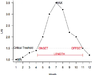
where LAI Min and Max represent minimum and maximum gridcell LAI over one year. The length of the growing season for each year was calculated as the number of months with an LAI value above this threshold; the onset is the first of these months and the dormancy is the last. Since part of the growing season occurs after the end of the year [38], we included the first three months of the following year in the calculations. Hence, the growing season offset can occur on the following year, having DOY higher than 365. Even when calculated monthly all results are presented in days (number of days passed until the end of the calculated month). The procedure was repeated for each gridcell, year and dataset. Mean length, onset and dormancy represent the average over the whole time period (Figure 1).
Figure 1. Growing season onset, dormancy (offset) and length calculation based on the
seasonal amplitude. A critical threshold value is calculated for each gridcell and each year based on the maximum and minimum Leaf Area Index (LAI).
In order to quantify the differences between the models and data we calculate the root mean square errors (Equation (2)) between each model and the satellite observations for each grid cell and all growing season variables, and the seasonal amplitude.
2.6. Temporal Trends
In order to calculate the temporal changes in annual average LAI and growing season length (GSL), linear trends were calculated for each gridcell for the whole time period. The values are presented as net change in both variables, in m2 m−2 and in days/year respectively. This approach has been used by other authors [34] giving important insights on the drivers of change.
3. Results
3.1. Mean LAI
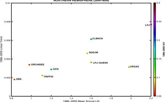
All of the models overestimate mean LAI, LAI trend and interannual variability (IAV) over the high-latitude Northern Hemisphere compared to the satellite observations (Figure 2). In general, models with the highest average LAI also have strong positive trends. This occurs regardless of whether the models use imposed or dynamic vegetation, or the number of PFTs implemented. Interestingly, models with a trend and average LAI closest to the satellite records, such as ORCHIDEE, OCN and TRIFFID have very different values of IAV, ranging from values similar to the satellite data up to 4 times higher. On the contrary, the most dissimilar models to the observations, such as LPJ and CLM4CN, have larger IAV.
Figure 2. Linear trend against average LAI for each model and satellite observations, with
IAV represented as colors. The data represents the whole high-latitude Northern Hemisphere (30°–90°) for the time period 1986–2005.
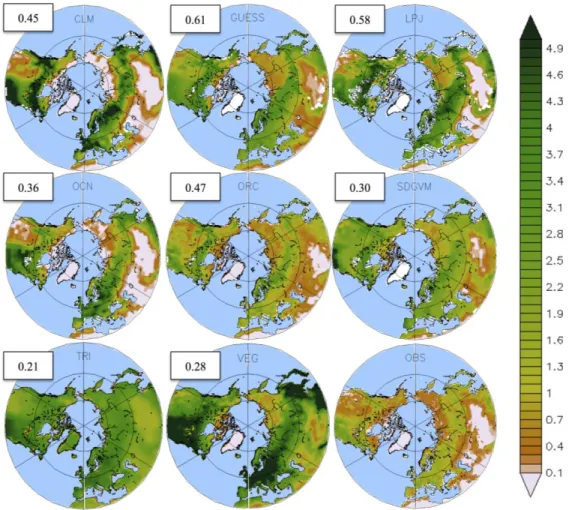
Looking at the spatial distribution of LAI, most of the models simulate the observed spatial distribution pattern (Figure 3). Peaks in LAI are evident over the boreal forest (55°–65°N) and the North American temperate forest (30°–55°N). The lowest values are found over the cold Gobi plateau and the Siberian Tundra. As noted above, there is a general overestimation of mean LAI in the models, relative to observations. LAI values range from 0 to 2.5 in the satellite data, while for the models they are as high as 5. Models and observations agree on values over the deserts and low-LAI regions but the differences
are higher (3–4) over the boreal region. As shown by spatial correlations, differences between satellite data and models are higher in VEGAS and TRIFFID, and smaller in LPJ and LPJ-GUESS (Figure 3). It is noteworthy that much of the discrepancies occur over evergreen vegetation, suggesting that the lack of regenerative vegetative states, fire and gap dynamics over this region lead to an overestimation of the number of fully grown trees on models, which ultimately means a much higher LAI than observed. However, satellite signal saturation—this is the inability of the satellite to distinguish between areas with high LAI- could be leading to an underestimation of LAI in dense forested areas such as the boreal forest, which might also account for the lower LAI over this area.
Figure 3. Spatially distributed annual mean LAI for 8 LSMs (1–8) and satellite observations
over the Northern Hemisphere (30°–90°N), for the period 1986–2005. Spatial correlations between each model and observations are given in the white boxes.
The seasonal amplitude patterns show large disagreements between the models and the satellite data (Figure 4). Most models overestimate the mean amplitude (RSME = 1.02–2.21), which is particularly evident over Europe and Eastern North America. The exception here is SDGVM, which displays little seasonality and performs better than the rest of the models in reproducing the satellite-derived observations. The RSME show that models using dynamic vegetation are less similar to observations than those using imposed vegetation. Regardless, most models correctly simulate the spatial variability of the seasonal amplitude; this is true for CLM, GUESS, OCN and VEGAS to some extent. TRIFFID shows almost no seasonality over this area, which is mainly driven by the omnipresence of the evergreen PFT over the Northern Hemisphere (not shown) (Figure 4).
Figure 4. Seasonal Amplitude in LAI for 8 LSMs and satellite observations for the Northern
Hemisphere (30°–90°N) for the period 1986–2005. Root mean square errors and spatial correlations between each model and the observations are given in the white boxes.
3.2. Growing Season
The growing season onset derived from LAI is broadly consistent across the models, with high correlations compared to the satellite data (>0.5) (Figure 5). In general the satellite observations show a later onset as latitude increases, remarkably similar to the thermal gradient. CLM, LPJ-GUESS, LPJ, SDGVM and, to a lesser extent, OCN, ORCHIDEE and VEGAS correctly reproduce this spatial pattern, as shown by the RSME and spatial correlations. This is not surprising as those models include a thermal limitation to photosynthesis and a snow scheme. TRIFFID shows no detectable onset above 50°N but has later values compared to the satellite below that threshold, likely due to the distribution of the evergreen PFT over the whole NH. Models that have the highest correlations with the satellite on the SA also show very similar values to the satellite on the onset, as shown by RSME (Figure 5).
Figure 5. Mean (1986–2005) growing season onset (day) for 8 LSMs and satellite
observations over the Northern Hemisphere (30°–90°N). Spatial correlations and root mean square errors between each model and the observations are given in the white boxes.
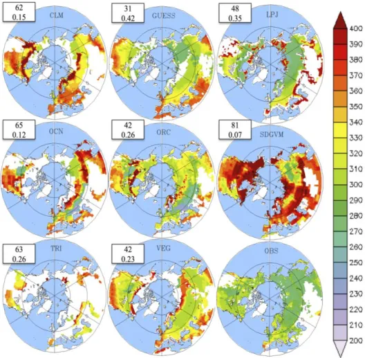
The discrepancies between the models and satellite observations are larger when considering the end of the growing season or dormancy (Figure 6). While the satellite data shows a latitudinal gradient, with the dormancy occurring earlier at higher latitudes, most models overestimate the dormancy day (RSME = 31–63). Out of the eight models, LPJ-GUESS, LPJ, ORCHIDEE and VEGAS have a similar dormancy distribution with minor discrepancies over the taiga and boreal forest, as shown by the spatial correlations. CLM, OCN and TRIFFID have patchy areas of agreement, while SDGVM has a much later dormancy than the satellite data. In some regions, particularly boreal deciduous forest, modeled dormancy can happen after the end of the year (DOY higher than 365). However, over these months the snow corrupts the satellite signal, leading to an underestimation of LAI. This partially explains why the dormancy date errors are larger than those of the onset.
All of the models predict a later dormancy date (day), particularly over the northern temperate region (30°–50°N) (Figure 6). This means that leaves in the models remain for longer than they should. However, the late dormancy is not in line with the vegetation photosynthetic activity. When the same methodology used to calculate the LAI-growing period was applied to gross primary productivity (GPP), we found that the dormancy began at 277 ± 7 days in the models, which is remarkably earlier than previously predicted by LAI (315 ± 10 days), even on the low-north latitudes
(287 ± 18). It is evident that all of the models keep inactive leaves for longer than they should, which does not have an impact on the C cycle but could potentially modify radiation and turbulent fluxes, therefore affecting planetary boundary layer dynamics.
Figure 6. Mean (1986–2005) growing season dormancy (day) for 8 LSMs and satellite
observations over the Northern Hemisphere (30°–90°N). Spatial correlations and root mean square errors between each model and the observations are given in the white boxes. DOYs above 365 represent DOYs of the following year.
There is a higher level of agreement in growing season length between the satellite data and the models than for dormancy dates (Figure 7). Surprisingly, the satellite observations display a very homogeneous length over regions > 50°N, with values between 120–150 days. Similar to the previous patterns, LPJ, LPJ-GUESS, CLM, ORCHIDEE and VEGAS have the highest agreement with the satellite data, as shown by the RSME and spatial correlations. Interestingly, the disagreement between models and observations occurs mostly over the lower latitudes of the Northern Hemisphere. OCN displays the same patchy agreement that shows on the onset and SDGVM displays the least agreement with an opposite GSL distribution. The length of the growing season has the highest error compared to the satellite data, where 6 out of 8 models display longer GSL, mostly driven by a late leaf shedding (Table 2).
When looking at the hemispheric mean values it is clear that all of the models overestimate the LAI, dormancy and length of the growing season (Table 2). Satellite LAI average for the Northern Hemisphere was 0.83, while LAI from the models varies between 0.98–2.16. Both growing season onset and dormancy
were later in all of the models, in some cases by more than a month. The effect of the late offset translates as an increased GSL, with values 9 to 180 days higher than the satellite data (Table 2). However, when the dormancy period is calculated based on GPP the modeled values become much closer to the observations, with an average GSL of 144 ± 15 days, compared to 184 days in the satellite data. This again suggests a decoupling between the active period of photosynthesis and leaves in the models.
Figure 7. Mean growing season length (1986–2005) in days for 8 LSMs and satellite
observations over the Northern Hemisphere (30°–90°N). Spatial correlations and root mean square errors between each model and the observations are given in the white boxes.
Table 2. Average LAI, growing season onset, dormancy and length for the Northern
Hemisphere for each model and the satellite observations. The values for dormancy and length based on GPP are presented in brackets.
Model LAI Onset (day) Dormancy (day) Length (days)
CLM 1.6 131 351 (288) 220 (164) LPJ_GUESS 1.6 125 314 (285) 189 (151) LPJ 2.2 130 319 (278) 189 (134) OCN 1.2 121 342 (268) 221 (142) ORCHIDEE 0.98 151 323 (268) 172 (134) SDGVM 1.56 122 374 (275) 252(145) TRIFFID 1.11 133 355 (274) 222(125) VEGAS 1.98 136 336 (277) 200 (139) LAI3g 0.83 111 295 184
3.3. Temporal Trends
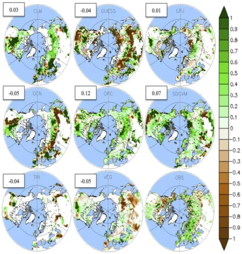
All models show a positive LAI trend in most of the Northern Hemisphere, which is consistent with the satellite observations (Figure 8). Nevertheless, there is little agreement on the spatial distribution of this phenomenon, with spatial correlation values between −0.05 and 0.12. In the satellite observation most of the greening occurs over 55°–90°N in Eurasia, while in models it is homogeneously distributed. More puzzling is the reduction of LAI in LPJ-GUESS, OCN and VEGAS, which could be explained by a decrease in precipitation over this region (not shown). As all models are forced using the same climate, consistent regional patterns must be driven by temperature or precipitation. The greening over the high latitudes occurs in all models and is driven by an increased temperature.
Figure 8. LAI linear trends over the period 1986–2005 for 8 LSMs and the satellite
observations. Spatial correlations between each model and the observations are given in the white boxes.
The models also show a general increase in the GSL albeit with a few areas where it decreases (Figure 9). However, similar to previous trends, there is little agreement over the spatial distribution. Clearly, models that perform better at calculating the GSL (both on the onset and dormancy) and average LAI more accurately reproduce observed linear trends (Figure 9). In most models, changes in the GSL match those of LAI. This is the case for CLM, OCN, ORCHIDEE, SDGVM and the satellite data, all of which use prescribed vegetation. LPJ, GUESS and VEGAS show an increased length over Eurasia and a decrease over North America, and their patterns resemble the precipitation trends for this
period (not shown). This discrepancy between LAI and GSL changes is difficult to explain but could be driven by vegetation shifts from deciduous to evergreen forests. Changes in the GSL in TRIFFID, while only occurring over a small area, match the observations.
Figure 9. Growing season length trends over the period 1986–2005 for 8 LSMs and the
satellite observations. Brown indicates an increase in the length of the growing season and green a decrease (days/year). In the white boxes, the values of the spatial correlation between each model and the satellite observations are given.
4. Discussion
The first important point to address is the validity of the satellite data. Satellite data does not represent true observations per se, but rather a model in itself. However, it is the closest product to observations, and available globally. It has been widely validated, but nevertheless there are some important issues that need to be considered. The satellite LAI product may have some problems detecting LAI in wintertime, since there is little sunlight in high latitudes. Sun angles are low and the satellite signals are heavily corrupted. Additionally snow cover affects reflection in winter and early spring. Hence, in the processing of any satellite data, there is a sun-angle cut-off. In these regions in the winter period
there is little or no data. This partially explains the difference with modeled dormancy dates. However, this does not matter since the soil during this time is frozen and the plants are not photosynthesizing, hence there are no changes in LAI. The methods used to detect the growing season will also ignore this period, since we are only interested in LAI when it starts to change, during the spring. In the region occupied by boreal forests, the same applies. The majority of the Boreal forests are photosynthetically inactive since they are covered in snow. They do however have green needles. These will begin to appear in late winter and early spring as radiation increases. The sun angles in some regions are above the processing cut-off limits and the satellite sensor will begin to register NDVI values. However the ground is still frozen and therefore there is no photosynthetic activity even if the air temperatures begin to rise above freezing during some hours of the day [36].
Over the boreal forest region (55°–65°N), all models exhibit an overestimation in LAI of 2–3 units compared to the satellite but also when compared with literature estimates [39]. We know that the satellite has an error precision of 20% at a pixel scale [40,41], field measurements have reported values around 2.7 ± 1.18 for the evergreen boreal forest [41] and 2.3 ± 0.6 for the deciduous forest [42]. The annual average over this region is around 1–2, which is inline with the satellite observations plus error. The average model values in this region are around 4, more similar to the expected maximum [39], than the expected mean (2.6–2.7). It seems that modeled LAI is higher all year round. These values are similar to the temperate forests, which suggests that having only one PFT for broadleaf forest might not be sufficient as is the case for TRIFFID, SDGVM and VEGAS. Moreover, models that include a wider range of PFTs, such as ORCHIDEE and LPJ-GUESS, are more similar to the satellite observations. Another possible explanation lies in the fact that models based on observed vegetation perform better than dynamic models. The lack of important ecosystem processes such as gap dynamics and fire, could be leading to the simulation of a mature forest state, which ultimately increases the PFT LAI.
There is great discrepancy in the calculation of the GSL with values that differ for more than a month, due to differences in the phenology module of each model. CLM4CN is one of the models that best predicts the GSL, since its LAI is derived from simulated leaf carbon and balanced with nitrogen [29]. More interestingly, models that use a thermal gradient to determine LAI (e.g., LPJ and LPJ-GUESS) [6,30] more accurately simulate the GSL than models with a more complex phenology, such as models where LAI is calculated from the leaf biomass (e.g., OCN [31], ORCHIDEE [32] and VEGAS [35]) or those that use a hydrological budget (e.g., SDGVM [32]). The exception is TRIFFID: while the model uses a thermal gradient for LAI [34], the introduction of a “chilling” phenology (leave shedding due to freezing) seems to overestimate the evergreen component in the Northern Hemisphere.
In spite of the differences in the phenology modules of the models, all predict an onset 15–20 days later than the satellite. Work by Jeong et al. [43] suggests that most models fail to calculate an adequate budburst due to the usage of mean air temperature threshold instead of accumulated heat variable, which generates better results. The authors also argue that the effect could come from the lack of representation of PFTs, which is consistent with our results–a higher number of PFTs leads to a better LAI and GSL representation. Another possible explanation is the overestimation of the effect of frozen soil thaw in the models.
All models predict a later dormancy, which occurs a month later than the satellite data. This happens due to all models having a constant leaf shedding over time once the temperature has reached a minimum certain threshold. While this might be true for the evergreen component, it creates a longer GSL for the
deciduous forest [44–46]. Moreover, the difference in the dormancy date between GPP and LAI clearly points out that models need to improve their LAI dormancy. While this might not have an impact on the C cycle, it could potentially alter the radiation and turbulent fluxes.
A longer growing season allows for a longer time of leaf growth, which explains the increasing LAI trend in the models, with the whole process being driven by temperature [47–49]. In most cases LAI plateaus at the maximum value, so if the growing season is longer, there are more days with maximum leaf area, which leads to a higher average value. This seems to be true for models with prescribed vegetation, although models that simulate dynamic vegetation follow the precipitation pattern more closely.
5. Conclusion
We compare LAI from eight different uncoupled LSMs against satellite data over the Northern Hemisphere, during the 1986–2005 period. This was achieved by calculating the mean LAI, seasonal amplitude and growing season variables (onset, dormancy an length). Our results show that all models overestimate LAI by 2–3 units, particularly over the boreal forest, relative to the satellite data and literature estimates. Models that include a high number of plant functional types (10–16) compare more favorably to the satellite data than those that only have a few (4–5). Models that calculate their phenology based on temperature perform better than those with complex photosynthetic modules. Likewise, models with prescribed vegetation more closely match observations than those that simulate it dynamically. Finally, all models overestimate the length of the by 4–40 days based on LAI compared with the observations, largely due to the dormancy date occurring 20–60 days later. This is inconsistent with the photosynthetic active period calculated by GPP, which was on average 3 months smaller. This highlights the need to improve the deciduous phenology in all models, particularly leaf shedding.
While vegetation models have developed a great deal, there is still a need for improvement. LAI is a key variable in all models and its correct representation, both temporarily and spatially, is key to predicting correct carbon fluxes. As the literature suggests, any overestimate in the length of the growing season and its trend is likely to affect albedo and have important effects on the radiation budget of the area. The satellite data represents a unique opportunity to test models against observational data and to determine where improvements can be made. Moreover, additional variables can be validated, allowing the identification of possible problems within the models.
Acknowledgments
We acknowledge the TRENDY-DGVM project that is responsible for all the data on DGVMs used in this work. We also thank Ranga Myneni for his valuable contribution and comments on the development of the paper and Xuhui Wang for is help on the methodology. The corresponding author also thanks the CONACYT-CECTI and the University of Exeter for their funding during the PhD studies. The National Center for Atmospheric Research is sponsored by the National Science Foundation.
Conflicts of Interest
References
1. Gomez-Peralta, D.; Oberbauer, S.F.; McClain, M.E.; Philippi, T.E. Rainfall and cloud-water interception in tropical montane forests in the eastern Andes of Central Peru. For. Ecol. Manag.
2008, 255, 1315–1325.
2. Running, S.W.; Coughlan, J.C. A general model of forest ecosystem processes for regional applications I. Hydrologic balance, canopy gas exchange and primary production processes. Ecol.
Model. 1988, 42, 125–154.
3. Bréda, N.J.J. Ground-based measurements of leaf area index: A review of methods, instruments and current controversies. J. Exp. Bot. 2003, 54, 2403–2417.
4. Knyazikhin, Y.; Martonchik, J.V.; Diner, D.J.; Myneni, R.B.; Verstraete, M.; Pinty, B.; Gobron, N. Estimation of vegetation canopy leaf area index and fraction of absorbed photosynthetically active radiation from atmosphere-corrected MISR data. J. Geophys. Res. 1998, 103, 32239–32256. 5. Landsberg, J.J.; Waring, R.H. A generalised model of forest productivity using simplified
concepts of radiation-use efficiency, carbon balance and partitioning. For. Ecol. Manag. 1997, 95, 209–228.
6. Sitch, S.; Smith, B.; Prentice, I.C.; Arneth, A.; Bondeau, A.; Cramer, W.; Kaplan, J.O.; Levis, S.; Lucht, W.; Sykes, M.T.; et al. Evaluation of ecosystem dynamics, plant geography and terrestrial carbon cycling in the LPJ dynamic global vegetation model. Glob. Change Biol. 2003, 9, 161–185. 7. Sitch, S.; Huntingford, C.; Gedney, N.; Levy, P.E.; Lomas, M.; Piao, S.L.; Betts, R.; Ciais, P.;
Cox, P.; Friedlingstein, P.; et al. Evaluation of the terrestrial carbon cycle, future plant geography and climate-carbon cycle feedbacks using five Dynamic Global Vegetation Models (DGVMs).
Glob. Change Biol. 2008, 14, 2015–2039.
8. Sitch, S.; Friedlingstein, P.; Gruber, N.; Jones, S.; Murray-Tortarolo, G.; Ahlstrom, A.; Doney, S.C.; Graven, H.; Heinze, C.; Huntingford, C.; et al. Trends and drivers of the regional-scale sources and sinks of carbon dioxide over the past two decades. Biogeosci. Discuss. 2013, in press.
9. Diaz, S.; Cabido, M. Plant functional types and ecosystem function in relation to global change.
J. Veg. Sci. 1997, 8, 463–474.
10. Diaz, S.; Cabido, M.; Casanoves, F. Plant functional traits and environmental filters at a regional scale. J. Veg. Sci. 1998, 9, 113–122.
11. Badeck, F.-W.; Bondeau, A.; Böttcher, K.; Doktor, D.; Lucht, W.; Schaber, J.; Sitch, S. Responses of spring phenology to climate change. New Phytol. 2004, 162, 295–309.
12. Buermann, W.; Dong, J.; Zeng, X.; Myneni, R.B.; Dickinson, R.E. Evaluation of the utility of satellite-based vegetation leaf area index data for climate simulations. J. Clim. 2001, 14, 3536–3550. 13. Maignan, F.; Bréon, F.-M.; Chevallier, F.; Viovy, N.; Ciais, P.; Garrec, C.; Trules, J.; Mancip, M.
Evaluation of a global vegetation model using time series of satellite vegetation indices. Geosci.
Model Dev. 2011, 4, 1103–1114.
14. Richardson, A.D.; Anderson, R.S.; Arain, M.A.; Barr, A.G.; Bohrer, G.; Chen, G.; Chen, J.M.; Ciais, P.; Davis, K.J.; Desai, A.R.; et al. Terrestrial biosphere models need better representation of vegetation phenology: Results from the North American carbon program site synthesis. Glob.
15. Randerson, J.T.; Hoffman, F.M.; Thornton, P.E.; Mahowald, N.M.; Lindsay, K.; Lee, Y.-H.; Nevison, C.D.; Doney, S.C.; Bonan, G.; Stöckli, R.; et al. Systematic assessment of terrestrial biogeochemistry in coupled climate–carbon models. Glob. Chang. Biol. 2009, 15, 2462–2484. 16. Prince, S.D. A model of regional primary production for use with coarse resolution satellite data.
Int. J. Remote Sens. 1991, 12, 1313–1330.
17. Myneni, R.B.; Ramakrishna, R.; Nemani, R.; Running, S.W. Estimation of global leaf area index and absorbed par using radiative transfer models. IEEE Trans. Geosci. Remote Sens. 1997, 35, 1380–1393.
18. Friedl, M.A.; Schimel, D.S.; Michaelsen, J.; Davis, F.W.; Walker, H. Estimating grassland biomass and leaf area index using ground and satellite data. Int. J. Remote Sens. 1994, 15, 1401–1420. 19. Chen, J.M.; Cihlar, J. Retrieving leaf area index of boreal conifer forests using Landsat TM
images. Remote Sens. Environ. 1996, 55, 153–162.
20. Green, E.P.; Mumby, P.J.; Edwards, A.J.; Clark, C.D.; Ellis, A.C. Estimating leaf area index of mangroves from satellite data. Aquat. Bot. 1997, 58, 11–19.
21. Prentice, I.C.; Bondeau, A.; Cramer, W.; Harrison, S.P.; Hickler, T.; Lucht, W.; Sitch, S.; Smith, B.; Sykes, M.T. Dynamic Global Vegetation Modeling: Quantifying Terrestrial Ecosystem Responses to Large-Scale Environmental Change. In Terrestrial Ecosystems in a Changing World; Canadell, J.G., Pataki, D.E., Pitelka, L.F., Eds.; Springer: New York City, NY, USA, 2007; pp. 175–192.
22. Anav, A.; Murray-Tortarolo, G.; Friedlingstein, P.; Sitch, S.; Piao, S.; Zhu, Z. Evaluation of land surface models in reproducing satellite Derived leaf area index over the high-latitude northern hemisphere. Part II: Earth system models. Remote Sens. 2013, 5, 3637–3661.
23. Xu, L.; Myneni, R.B.; Chapin, F.S. III; Callaghan, T.V.; Pinzon, J.E.; Tucker, C.J.; Zhu, Z.; Bi, J.; Ciais, P.; Tømmervik, H.; et al. Temperature and vegetation seasonality diminishment over northern lands. Nat. Clim. Change 2013, doi: 10.1038/nclimate1836.
24. Anav, A.; Menut, L.; Khvorostyanov, D.; V ovy, N. Impact of tropospheric ozone on the Euro-Mediterranean vegetation. Glob. Chang. Biol. 2011, 17, 2342–2359.
25. Yang, W.; Tan, B.; Huang, D.; Rautiainen, M.; Shabanov, N.V.; Wang, Y.; Privette, J.L.; Huemmrich, K.F.; Fensholt, R.; Sandholt, I.; et al. MODIS leaf area index products: From validation to algorithm improvement. IEEE Trans. Geosci. Remote Sens. 2006, 44, 1885–1898. 26. Gao, F.; Morisette, J.T.; Wolfe, R.E.; Ederer, G.; Pedelty, J.; Masuoka, E.; Myneni, R.; Tan, B.;
Nightingale, J. An algorithm to produce temporally and spatially continuous MODIS-LAI time series. IEEE Geosci. Remote Sens. Lett. 2008, 5, 60–64.
27. Ganguly, S.; Schull, M.A.; Samanta, A.; Shabanov, N.V.; Milesi, C.; Nemani, R.R.; Knyazikhin, Y.; Myneni, R.B. Generating vegetation leaf area index earth system data record from multiple sensors. Part 1: Theory. Remote Sens. Environ. 2008, 112, 4333–4343. 28. Ganguly, S.; Nemani, R.R.; Zhang, G.; Hashimoto, H.; Milesi, C.; Michaelis, A.; Wang, W.;
Votava, P.; Samanta, A.; Melton, F.; et al. Generating global Leaf Area Index from Landsat: Algorithm formulation and demonstration. Remote Sens. Environ. 2012, 122, 185–202.
29. Oleson, K.W.; Lawrence, G.B.; Flanner, M.G.; Kluzek, E.; Levis, P.J.S.; Swenson, S.C.; Thornton, E.; Feddema, J.; Heald, C.L.; Lamarque, J.; et al. Technical Description of Version 4.0
30. Smith, B.; Prentice, I.C.; Sykes, M.T. Representation of vegetation dynamics in the modelling of terrestrial ecosystems: Comparing two contrasting approaches within European climate space.
Glob. Ecol. Biogeogr. 2001, 10, 621–637.
31. Zaehle, S.; Friend, A.D. Carbon and nitrogen cycle dynamics in the O-CN land surface model: 1. Model description, site-scale evaluation, and sensitivity to parameter estimates. Glob. Biogeochem.
Cy. 2010, 24, doi: 10.1029/2009GB003521
32. Krinner, G.; Viovy, N.; de Noblet-Ducoudré, N.; Ogée, J.; Polcher, J.; Friedlingstein, P.; Ciais, P.; Sitch, S.; Prentice, I.C. A dynamic global vegetation model for studies of the coupled atmosphere-biosphere system. Glob. Biogeochem. Cy. 2005, 19, doi: 10.1029/2003GB002199. 33. Woodward, F.I. Vegetation-climate feedbacks in a greenhouse world. Philos. Trans. R. Soc. Lond.
B Biol. Sci. 1998, 353, 29–39.
34. Cox, P. Description of the TRIFFID Dynamic Global Vegetation Model; Techinal Note 24; Met Office: Berks, UK, 2001. Available online: http://climate.uvic.ca/model/common/HCTN_24.pdf (accessed on 23 April 2013).
35. Zeng, N.; Qian, H.; Roedenbeck, C.; Heimann, M. Impact of 1998–2002 midlatitude drought and warming on terrestrial ecosystem and the global carbon cycle. Geophys. Res. Lett. 2005, 32, doi: 10.1029/2005GL024607.
36. Zhu, Z.; Bi, J.; Pan, Y.; Ganguly, S.; Anav, A.; Xu, L.; Samanta, A.; Piao, S.; Nemani, R.R.; Myneni, R. B. Global data sets of vegetation Leaf Area Index (LAI)3g and fraction of Photosynthetically Active Radiation (FPAR)3g derived from Global Inventory Modeling and Mapping Studies (GIMMS) Normalized Difference Vegetation Index (NDVI3g) for the period 1981 to 2011. Remote Sens. 2013, 5, 927–948.
37. Piao, S.; Friedlingstein, P.; Ciais, P.; Viovy, N.; Demarty, J. Growing season extension and its impact on terrestrial carbon cycle in the Northern Hemisphere over the past 2 decades. Glob.
Biogeochem. Cy. 2007, 21, doi: 10.1029/2006GB002888.
38. Zhang, P.; Anderson, B.; Barlow, M.; Tan, B.; Myneni, R.B. Climate-related vegetation characteristics derived from Moderate Resolution Imaging Spectroradiometer (MODIS) leaf area index and normalized difference vegetation index. J. Geophys. Resea.-Atmos. 2004, 109, doi:10.1029/2004JD004720.
39. Asner, G.P.; Scurlock, J.M.O.; Hicke, J.A. Global synthesis of leaf area index observations: Implications for ecological and remote sensing studies. Glob. Ecol. Biogeogr. 2003, 12, 191–205. 40. Berterretche, M.; Hudak, A.T.; Cohen, W.B.; Maiersperger, T.K.; Gower, S.T.; Dungan, J.
Comparison of regression and geostatistical methods for mapping Leaf Area Index (LAI) with Landsat ETM+ data over a boreal forest. Remote Sens. Environ. 2005, 96, 49–61.
41. Wang, Y.; Woodcock, C.E.; Buermann, W.; Stenberg, P.; Voipio, P.; Smolander, H.; Häme, T.; Tian, Y.; Hu, J.; Knyazikhin, Y.; et al. Evaluation of the MODIS LAI algorithm at a coniferous forest site in Finland. Remote Sens. Environ. 2004, 91, 114–127.
42. Bonan, G.B. Importance of Leaf Area Index and forest type when estimating photosynthesis in boreal forests. Remote Sens. Environ. 1993, 43, 303–314
43. Jeong, S.-J.; Ho, C.-H.; Gim, H.-J.; Brown, M.E. Phenology shifts at start vs. end of growing season in temperate vegetation over the Northern Hemisphere for the period 1982–2008. Glob.
44. Hickler, T.; Smith, B.; Prentice, I.C.; Mjöfors, K.; Miller, P.; Arneth, A.; Sykes, M.T. CO2
fertilization in temperate FACE experiments not representative of boreal and tropical forests.
Glob. Change Biol. 2008, 14, 1531–1542.
45. Norby, R.J.; Sholtis, J.D.; Gunderson, C.A.; Jawdy, S.S. Leaf dynamics of a deciduous forest canopy: No response to elevated CO2. Oecologia 2003, 136, 574–584.
46. Iivonen, S.; Kaakinen, S.; Jolkkonen, A.; Vapaavuori, E.; Linder, S. Influence of long-term nutrient optimization on biomass, carbon, and nitrogen acquisition and allocation in Norway spruce. Can.
J. For. Res. 2006, 36, 1563–1571.
47. Lucht, W.; Prentice, I.C.; Myneni, R.B.; Sitch, S.; Friedlingstein, P.; Cramer, W.; Bousquet, P.; Buermann, W.; Smith, B. Climatic control of the high-latitude vegetation greening trend and pinatubo effect. Science 2002, 296, 1687–1689.
48. De Jong, R.; Verbesselt, J.; Zeileis, A.; Schaepman, M. Shifts in global vegetation activity trends.
Remote Sens. 2013, 5, 1117–1133.
49. Mao, J.; Shi, X.; Thornton, P.; Hoffman, F.; Zhu, Z.; Myneni, R. Global latitudinal-asymmetric vegetation growth trends and their driving mechanisms: 1982–2009. Remote Sens. 2013, 5, 1484–1497.
© 2013 by the authors; licensee MDPI, Basel, Switzerland. This article is an open access article distributed under the terms and conditions of the Creative Commons Attribution license (http://creativecommons.org/licenses/by/3.0/).