HAL Id: hal-02171334
https://hal-enpc.archives-ouvertes.fr/hal-02171334
Submitted on 10 Jul 2019HAL is a multi-disciplinary open access
archive for the deposit and dissemination of sci-entific research documents, whether they are pub-lished or not. The documents may come from teaching and research institutions in France or abroad, or from public or private research centers.
L’archive ouverte pluridisciplinaire HAL, est destinée au dépôt et à la diffusion de documents scientifiques de niveau recherche, publiés ou non, émanant des établissements d’enseignement et de recherche français ou étrangers, des laboratoires publics ou privés.
Imaging non-Brownian particle suspensions with X-ray
tomography: application to the microstructure of
Newtonian and visco-plastic suspensions
Stephanie Deboeuf, Nicolas Lenoir, David Hautemayou, Michel Bornert, F.
Blanc, Guillaume Ovarlez
To cite this version:
Stephanie Deboeuf, Nicolas Lenoir, David Hautemayou, Michel Bornert, F. Blanc, et al.. Imaging non-Brownian particle suspensions with X-ray tomography: application to the microstructure of Newtonian and visco-plastic suspensions. Journal of Rheology, American Institute of Physics, 2017, 62 (2), pp.643. �10.1122/1.4994081�. �hal-02171334�
HAL Id: hal-02171334
https://hal-enpc.archives-ouvertes.fr/hal-02171334
Submitted on 10 Jul 2019HAL is a multi-disciplinary open access
archive for the deposit and dissemination of sci-entific research documents, whether they are pub-lished or not. The documents may come from teaching and research institutions in France or abroad, or from public or private research centers.
L’archive ouverte pluridisciplinaire HAL, est destinée au dépôt et à la diffusion de documents scientifiques de niveau recherche, publiés ou non, émanant des établissements d’enseignement et de recherche français ou étrangers, des laboratoires publics ou privés.
Imaging non-Brownian particle suspensions with X-ray
tomography: application to the microstructure of
Newtonian and visco-plastic suspensions
Stephanie Deboeuf, Nicolas Lenoir, David Hautemayou, Michel Bornert,
Guillaume Ovarlez
To cite this version:
Stephanie Deboeuf, Nicolas Lenoir, David Hautemayou, Michel Bornert, Guillaume Ovarlez. Imag-ing non-Brownian particle suspensions with X-ray tomography: application to the microstructure of Newtonian and visco-plastic suspensions. Journal of Rheology, 2017. �hal-02171334�
1 2 3 4 5 6 7 8 9 10 11 12 13 14 15 16 17
Imaging
non-Brownian particle suspensions with X-ray
tomography:
application
to the microstructure of Newtonian and visco-plastic
suspensions
S. Deboeuf∗
Sorbonne Universit´es, UPMC Univ. Paris 06, CNRS, UMR 7190, Institut Jean Le Rond dAlembert, 75005 Paris, France
N. Lenoir
PLACAMAT, UMS 3626 CNRS-Univ. de Bordeaux, Pessac, France D. Hautemayou and M. Bornert
Universit´e Paris-Est, Laboratoire Navier (UMR 8205) CNRS, ENPC, IFSTTAR, F-77420 Marne-la-Vall´ee, France
F. Blanc
CNRS-University of Nice, LPMC-UMR 7336, 06108 Nice, France G. Ovarlez
Univ. Bordeaux, CNRS, Solvay, LOF, UMR 5258, F-33608 Pessac, France
(Dated: September 29, 2017)
Abstract
A key element in the understanding of the rheological behaviour of suspensions is their mi-crostructure. Indeed, the spatial distribution of particles is known to depend on flow history in suspensions, which has an impact on their macroscopic properties. These micro-macro couplings appeal for the development of experimental tools allowing for the rheological characterization of a suspension and the imaging of particles. In this paper, we present the technique we developed to image in three dimensions the microstructure of suspensions of non-Brownian particles, using X-ray computed tomography and sub-voxel identification of particle centers. We also give exam-ples of the information we can get in the case of Newtonian and visco-plastic suspensions, referring to Newtonian and visco-plastic suspending fluid. We compute three dimensional pair distribu-tion funcdistribu-tions and show that it is possible to get a nearly isotropic microstructure after mixing. Under shear, this microstructure becomes anisotropic in the shear plane (velocity-velocity gradi-ent plane), whereas it is almost isotropic in the two other planes (velocity-vorticity and velocity gradient-vorticity planes). When changing the plane of shear (from a squeeze flow to a rotation flow), the microstructure reorganizes to follow this change of shear plane. It is known that for Newtonian suspensions the anisotropy is independent on the shear rate; we show here that for a visco-plastic suspension it depends on it. Finally, we study the structuration close to boundaries and we evidence some particle alignment along both solid surfaces and, more surprisingly, along free interfaces.
I. INTRODUCTION
19
Many flowing materials encountered in nature (landslides, debris or lava flows, ...) or
20
raw materials produced in industry (concrete, batter, ...) are mixtures of dispersed solids in
21
a liquid. These systems are composed of a wide range of materials of various sizes, which
22
makes them complex to understand. In order to predict the behaviour and optimize the use
23
of these suspensions, a useful step is to identify model systems capable of reproducing the
24
phenomenology of interest and to understand the rheology of controlled suspensions. When
25
length scales between the coarser and the finer dispersed particles of a suspension are well
26
separated, a possible model system is a visco-plastic suspension of solid particles, referring to
27
a visco-plastic suspending fluid, i.e. of nonlinear viscosity with a yield stress. Indeed, from a
28
rheological point of view, a fresh concrete can be considered as coarse particles (sand, gravel)
29
suspended in a visco-plastic fluid (cement paste) [1, 2]. Even more simply, one can consider
30
a Newtonian suspension of solid particles as a model system, referring to a Newtonian
31
suspending fluid [3]. A lot can indeed be learnt from such materials: studying first the
32
interactions of multiple particles in a linear (Newtonian) fluid is crucial to understand their
33
interaction in a nonlinear medium [4, 5]. This knowledge can then be applied to materials
34
closer to applications such as cementitious materials [2, 6].
35
A key element in the understanding of the rheological behaviour of suspensions is their
36
microstructure [7, 8]. Indeed, the spatial distribution of particles in suspensions is known to
37
depend on the flow history – an anisotropic distribution is induced by shear –, which has an
38
impact on their properties [7, 9–14] – an anisotropic microstructure is at the origin of normal
39
stress differences and of viscosity variations during transient regimes. These micro-macro
40
couplings between microstructure and flow appeal for the development of experimental and
41
numerical tools allowing for the characterization of the rheology of a suspension and the
42
imaging of its microstructure. A lot of numerical studies used Stokesian dynamics equations
43
[8, 15–18]. The existing experimental techniques efficient for non-Brownian suspensions are
44
all based on optics. Non-Brownian particles are indeed too large to use scattering techniques
45
such as X-ray scattering or coherent diffraction imaging. For non transparent particles in a
46
transparent fluid, it is nevertheless possible to image the microstructure only near the free
47
surface [10] or near a transparent boundary. As we will demonstrate here, the proximity of a
48
boundary (a solid wall or a free interface) influences strongly the microstructure and makes
it different from the one in the bulk. The bulk microstructure can be obtained only for
50
specific suspensions, where particles and the fluid have the same optical index; a laser sheet
51
can then be used to light a plane embedding a fluorescent stain so as to visualize and identify
52
particles in two dimensions (2D) [11, 12]. Obtaining a three dimensional microstructure
53
then implies to displace the position of the laser sheet. Confocal microscopy can also be used
54
for micron-sized particles [18, 19], submitted to Brownian diffusion, that is in competition
55
with shear flow, quantified by the Peclet number (being the ratio of hydrodynamic over
56
thermal forces). Here we choose to use non intrusive X-ray techniques as a promising tool
57
to image in the bulk suspensions in three dimensions (3D).
58
In this paper, we present the technique we developed to image in 3D the microstructure
59
of suspensions of non-Brownian particles, using X-ray computed tomography (CT) and then
60
identifying by image analysis the particle centers with a sub-voxel resolution. All the details
61
to duplicate our technique are given. We give examples of the information we can get in the
62
case of Newtonian and visco-plastic suspensions. We compute 3D pair distribution functions
63
(pdf) and show that it is possible to get a nearly isotropic microstructure after mixing. Under
64
shear, this microstructure becomes anisotropic in the shear plane (velocity-velocity gradient
65
plane), whereas it is nearly isotropic in the two other planes (velocity-vorticity and velocity
66
gradient-vorticity planes). When changing the plane of shear (from a squeeze flow to a
67
rotation flow), the microstructure reorganizes to follow this change of shear plane. While it
68
is known that for Newtonian suspensions the anisotropy is independent on the shear rate, we
69
show that for a visco-plastic suspension it depends on it. Finally, we study the structuration
70
close to boundaries and we evidence particle alignment along both solid surfaces and more
71
surprisingly along free interfaces.
72
In Sec II, we present the principles of our study and we provide the details on the studied
73
suspensions and the set-up. Sec III is devoted to the X-ray tomography technique and to the
74
method we developed to identify particles center and compute pair distribution functions.
75
In Sec IV, we present various examples of the microstructure of Newtonian and visco-plastic
76
suspensions.
a) b) c)
FIG. 1. X-ray computed micro-tomography set-up (a and b) and dedicated parallel plates set-up (c). The sketch (a) shows the X-ray source (in white), the imaging device (in green), the rotation (in red) and translation (in blue) stages and the parallel plates set-up (in yellow).
II. MATERIALS AND METHODS
78
A. Goals and general principles
79
Our goal is to get enough information at the microstructure scale to guide developments
80
of micro-mechanical models for complex suspensions rheology. Thus, we need to image
81
particles in a flow cell and to characterize their spatial distribution for various flow histories.
82
Our system made of a suspension in a rheometrical set-up should allow for the
investiga-83
tion from small to large space scales, from the length of the dispersed particles to the whole
84
suspension. The flow cell should be large enough to be representative of a macroscopic shear
85
flow, to ensure that the material exhibits a bulk behaviour not influenced by finite size or
86
non local effects [20], and to get enough statistics for studying the microstructure. This
87
leads us to choose a rheometer equipped with a parallel plates geometry (Fig. 1c). In the
88
same time as doing rheology, we want to image the microstructure in 3D, even in the case
89
of non matched optical index materials. This leads us to use X-ray CT imaging, which is
90
efficient for many suspensions and geometries, as long as there is enough X-ray absorption
91
contrast between particles and the fluid.
92
The sample to image is placed on a rotating stage between an X-ray source and a 2D
93
imaging device (Fig. 1), which monitors the transmission of X-rays through the sample. In
94
our case, the imaging device was a PaxScan2520V flat panel detector from Varian, made of
95
a CSI scintillator and a matrix of 1920x1536 pixels (among which 1840x1456 are effective),
96
with a pixel width of 127 µm. This provides a 2D radiograph, accounting for the total
absorption along linear paths through the sample. A series of 2D radiographs for different
98
rotation angles of the sample (typically over 360◦ in a lab X-ray CT device) then allows for
99
the reconstruction of the 3D map of absorption coefficients [21–23]. If particles and the fluid
100
do not have the same absorption coefficient, we can finally achieve to detect the particles.
101
This map is discretized over elementary volumes called voxels (i.e. volumic pixels). The
102
achievable minimum voxel size is given by the ratio of the size of the imaged sample over
103
the number of pixels in the detector width. The typical width of the CCD detectors used
104
for X-ray CT is about 2000 pixels. Noting D, the diameter of the parallel plates geometry,
105
the minimum possible voxel size is D/2000. To identify precisely the particles center, their
106
diameter d should be at least 10 voxels, i.e. d & D/200. The gap size H between the plates
107
in the parallel plates geometry should contain at least 10 particles to avoid some finite size
108
effects, i.e. H & D/20, which is compatible with the study here but limits the possible
109
aspect ratios diameter/gap of the geometry to D/H . 20. We will show later that our
110
home-made algorithms allow us to refine particle centers positions at a sub-voxel resolution
111
of an order of d/100, that ultimately allows for a fine characterization of the microstructure.
112
Here (Fig. 2a), the diameter of the parallel plates geometry id D = 2cm, the gap of the
113
geometry is H = 2mm, the size of particles d is between 100µm and 200µm, the size of
114
voxels is 12µm and the final accuracy on the particles centers in most cases presented here
115
is 6µm, but it can be decreased down to 1µm if necessary.
116
X-ray CT imaging may demand a non negligible time for scanning. The time for one scan
117
depends of the X-ray set-up, the suspension properties and the chosen spatial resolution
(X-118
ray flux, number of radiographs, time exposure, ...). With our X-ray CT device and the
119
chosen spatial resolution, the whole sample can be scanned in 20 minutes but with a poor
120
signal-to-noise ratio. The results presented here are obtained from 1 hour-scan in order to
121
enhance the image quality. During the time of a scan, particles must not move within the
122
suspending fluid (i.e. displacement less than 1 voxel or even less, if subvoxel accuracy is
123
expected). This leads us to use first a visco-plastic fluid as a suspending fluid ensuring that
124
particles do not move as long as stresses are smaller than the yield stress. Then we apply to
125
our suspension a given shear history, then stop the flow and image the material at rest with
126
a frozen structure, which is supposed to be close to the structure under flow. The underlying
127
hypothesis is that relaxation of the microstructure at rest is negligible. This flow-arresting
128
technique was already used before for Brownian suspensions [18]. In a second time, we
FIG. 2. (a) Scheme of the parallel plates set-up: D and H are the plates diameter and gap, d is the particles diameter, Ω and ϑ are the rotational and translational velocities of the top plate. (b) Schemes of the rotational and squeeze shear flows: the suspension velocity uθ(r, z) and ur(r, z) are
aligned with the azimuthal and radial directions respectively. (c) A picture processed from X-ray slices showing the rough surface with grooves of the set-up’s plates.
succeed to use a Newtonian suspension with density-matched particles and fluid, to avoid
130
any buoyancy effects at rest. In principe, various types of suspensions may be imaged and
131
studied with our technique, as soon as particles or suspended objects do not move during the
132
time of a X-ray scan. For particles as small as a few µm, Brownian fluctuations may call for
133
even quicker X-ray micro-tomograph (e.g. Synchrotron source). In terms of concentration
134
of particles, we have successfully image in 3D suspensions at solid fractions as high as 50%
135
and it should be possible to go even higher.
136
TABLE I. Properties of particles and fluids used for the Newtonian and the visco-plastic suspen-sions: average diameter d of particles, viscosity η of the Newtonian fluid, elastic shear modulus G0, yield stress τy and consistency K of the visco-plastic fluid and density ρ of the fluid and
density-matched particles. PMMA Newtonian Density
d(µm) η(Pa.s) ρ 170 ± 12 1.3 1.19
PS Yield stress Density
d(µm) G0(Pa) τ
y(Pa) K (Pa.s0.5) ρ
B. Suspensions of non-Brownian particles
137
Two suspensions are studied here (Table I): one is composed of poly(methyl
methacry-138
late) (PMMA) spheres in a Newtonian fluid and the other is composed of polystyrene
139
(PS) spheres in a visco-plastic fluid. In both cases, particles and suspending fluids are
140
density-matched to avoid any buoyancy effects. The PMMA particles average diameter
141
is 170µm±12µm and the PS particles average diameter is 138µm±8µm. These diameters
142
were measured from optical pictures of bead samples. With such a size, particles are
non-143
Brownian and supposed to be non-colloidal. For all of experiments presented in this work,
144
the solid fraction φ of the suspensions was observed to be uniform within our rheological
145
set-up.
146
The Newtonian suspending fluid is an acrylic double matching liquid from Cargille Lab.
147
Its density is 1.19 and its viscosity 1300 mPa.s at 25◦C. The natural contrast of X-ray
148
absorption between particles and the fluid is sufficient to separate them in final X-ray CT
149
images.
150
The visco-plastic fluid, of density 1.05, is a concentrated emulsion of aqueous drops
151
dispersed at a 77.5% volume fraction (volume of dispersed phase over total volume) in a
152
continuous oily phase. Surfactant SPAN80 is added in dodecane oil at 7.5% in mass (SPAN80
153
mass over dodecane mass) and iodine sodium salt is added in water at 15% in mass (NaI
154
mass over H2O mass) to stabilize the emulsion and enhance contrast for X-ray imaging. The
155
droplets size is of order of 1µm, much smaller than the particles size. This ensures that the
156
emulsion is seen as a continuous material – a visco-plastic fluid – by the particles [2, 4, 5].
157
The behaviour of the visco-plastic fluid is well described by a Herschel-Bulkley law, relating
158
the shear stress τ to the shear rate ˙γ, with τy = 26Pa and K = 5.1Pa.s0.5:
159
τ = τy + K ˙γ0.5, if τ ≥ τy, (1)
valid in the steady flow regime, i.e. for stresses larger than the yield stress τy. The elastic
160
contribution to its behaviour is accounted for by the elastic shear modulus G0 = 250Pa.
161
More details on the rheology of both background (Newtonian and visco-plastic) fluids,
162
with and without particles, in [5] and [24] respectively.
a) b)
c)
FIG. 3. X-ray radiograph corresponding to the transmitted intensity of X-rays through the sample (the visco-plastic suspension) along one linear path (a), reconstructed horizontal slice encoding for X-ray absorption of voxels in the shear cell at a solid fraction φ ' 35% (b) and zoom of this slice (c) corresponding to the white rectangle drawn in (b). The scale bar drawn in (c) is 1mm long.
C. X-ray microtomography
164
In this study, we used the X-ray microtomography device of Laboratoire Navier, made
165
up of an Ultratom scanner designed and assembled by RX Solutions (Annecy, France) on
166
the basis of the specific requests of Laboratoire Navier. Using the commercial software Xact
167
developed by this company, based on the filtered retroprojection algorithm adapted to
cone-168
beam geometry [25], 3D images encoding for the X-ray absorption field are reconstructed
169
from the recorded 2D radiographs. Consistently with the definition of the final 3D images,
170
1440 radiographs have been recorded over 360◦. Note that for each rotation angle, 6
radio-171
graphs (with an exposure time for one radiograph of 1/3s) have been averaged to improve
172
the signal to noise ratio. The final 3D images had a resolution of 12µm and a definition of
173
1840x1840x170 voxels.
174
One of the advantages of this technique is that the spatial resolution can be isotropic,
con-175
trary to other scanning techniques, such as confocal microscopy, laser scanning or refractive
176
index matched scanning [12, 26–29]. This allows to get information on the microstructure
177
with the same accuracy in all planes. Figure 3 shows one example of a 2D radiograph of the
178
visco-plastic suspension confined between the two parallel plates and 12µm-thick horizontal
179
slices of the reconstructed 3D image for a solid fraction φ ' 35%.
D. Dedicated rheological set-up
181
The suspension is sheared at the macroscopic scale in a parallel plates geometry (Fig. 2a)
182
of diameter D = 2cm and gap H = 2mm (aspect ratio D/H = 10), controlled by a rheometer
183
(Kinexus, Malvern). The plates of the shear cell (Fig. 2c) are made rough to prevent slipping
184
of the suspension at solid boundaries. They have been treated as follow: each PMMA plate
185
was roughened thanks to sand-paper of roughness size 150µm, then a grid pattern of grooves
186
was imprinted thanks to a file with an edge (triangular lime). In the following, we will
187
compare some results with smooth PMMA plates and roughened PMMA plates.
188
To image a sample in 3D, 2D radiographs have to be recorded for many different view
189
angles, which means that X-rays have to be allowed to propagate through the sample for
190
all directions nearly perpendicular to the rotation axis, which would not be possible with
191
a standard rheometer (its body would block X-rays when placed between the source and
192
the detector). This leads us to build a dedicated parallel plates set-up, made of PMMA to
193
ensure a low X-ray absorption by the set-up (Fig. 1c). This set-up can be inserted in the
194
rheometer for shearing the material and characterizing its rheological response. After a given
195
shear history in the rheometer, it can then be blocked thanks to a chuck, removed from the
196
rheometer and carefully moved (to avoid any disturbance) to the X-ray CT set-up, where it
197
is put on the rotating stage for imaging. During the whole duration of X-ray imaging, the
198
parallel plates set-up is blocked. We checked that our ex-situ experiments (moved from the
199
rheometer to the X-ray CT set-up) lead to the same results as in-situ ones (for which both
200
shear and imaging are on the spot).
201
In a parallel plates geometry, when rotation is imposed to the top plate at a rate Ω
202
while keeping fixed the bottom plate (Fig. 2b), the force balance equation and boundary
203
conditions (no slip at the two plates) predict a simple shear of the fluid in the orthoradial
204
plane (θz), the single non-zero value of the shear rate tensor being:
205
˙γ(r) = 2dzθ(r) = Ωr/H, (2)
with an azimuthal velocity:
206
uθ(r, z) = Ωzr/H, (3)
(r, θ, z) being the cylindrical coordinates [30]. The rotational shear is not homogeneous but
207
depends linearly on the radial direction r. This analysis holds not only for Newtonian fluids,
but for complex fluids too.
209
In the same geometry of parallel plates, a squeeze flow can be imposed by translating
210
vertically one plate at a velocity ϑ (Fig. 2b). It can be approximated by a simple shear
211
flow in the radial plane (rz), in the case of a large aspect ratio D/H and of no slip at
212
solid boundaries [30–32]. In this case, the shear rate ˙γ(r, z) = 2dzr(r, z) is inhomogeneous
213
and a priori unknown: it depends on the rheology of the fluid of interest. Nevertheless,
214
a convenient approximation of the maximal shear rate, valid for a Newtonian fluid in the
215
lubrication approximation, is:
216
˙γ = 3Dϑ/(2H2). (4)
Note that by symmetry, the shear has a different sign in the upper and lower part of the
217
suspension through the central surface at z = 0.
218
In order to shear the material in a parallel plates geometry, it is first poured on the
219
bottom plate, then it is squeezed by the top plate to reach the required gap. So even if the
220
interest is in a rotational shear, the material generally experiences first a squeeze flow during
221
the loading of the fluid in the geometry, which might affect its initial state. That is why in
222
the following, we will investigate the impact of both flows on the suspension microstructure.
223
III. IMAGE ANALYSIS
224
An accurate identification of particle centers from the obtained 3D images is crucial for the
225
computation of pair vectors and pair distribution functions to characterize the microstructure
226
of the suspension. Thus, we choose to develop home-made algorithms to be able to identify
227
particles center at a sub-voxel resolution.
228
In all the text, the 3D images I we work with are fields of absorption coefficients encoded
229
as intensity levels without unit measurement. In practice, 16 bits images have been used
230
(grey levels between 0 and 216-1).
231
Figure 4 shows the typical greylevel profile of a particle: grey levels of all voxels in the
232
neighborhood of a particle are plotted against the distance r to the voxel considered to be
233
its center. Assuming the density of the particles to be uniform, one would have expected a
234
Heaviside-like shape for such plots, with a uniform grey level for r lower than the particle
235
radius (of the order of 6 voxels), corresponding to the absorption coefficient of PMMA or
236
PS, and another (larger) uniform grey level for larger r, corresponding to the absorption of
a) r ✁✂✄ ✲☎ ✆ ✝✞ ✵ ✺ ✶ ✟ ■ ★✠ ✡ ✷ ✸ ☛ ☞ ✻ b) ✌✍✎✏ ✑ ✒✓ ✔ ✕✖ ✗ ✘ ✙ ✚ ✛ ❢ ✜ ✢✣ ✥ ✦ ✧ ✩ ✪
FIG. 4. Absorption levels (without unit measurement, included between 0 and 216− 1) of voxels
over one particle and its close neighbourhood in the visco-plastic suspension at a solid fraction φ '40%, as a function of the distance r to its center, from the raw and filtered images I (a) and If (b)
the fluid.
238
Actual profiles first differ from ideal profiles because of natural random image noise, which
239
cannot be avoided, especially if fast imaging conditions are required. Such fluctuations are
240
indeed observed near r = 0, up to a distance of about 2 to 3 voxels, where grey levels are
241
essentially uniform on average but fluctuate randomly.
242
The second discrepancy with respect to the ideal situation takes the form of a gradual
243
increase of the average grey levels for r varying from about 3 to 7 voxels. While there
244
are still fluctuations associated to natural image noise, the smooth progressive increase of
245
the average grey level is due to the limited spatial resolution of the CT imaging device.
246
Indeed the grey level of a given voxel in the reconstructed image should be considered as
247
a spatial convolution of the physical absorption coefficient of the material (relative to the
248
spectrum of the polychromatic X-ray beam) with some kernel of small finite size. This
249
kernel characterizes the resolving power of the imaging system. For CT imaging systems,
250
it is sensitive to various parameters, such as the finite spot size of the X-ray source (which
251
can be evaluated to be about 8 µm for our imaging conditions), diffusion effects of the
252
scintillator, fill factor of the pixel matrix, blurring effects of electronic device,... A more
253
detailed discussion can be found in [33]. In the present setup, and considering the grey level
254
profile presented in figure 4, the radius of this kernel is likely to be of the order of 2 to 3
TABLE II. Values of the parameters `noise, rneigh, rmin and rsym used for image analyses, with d,
the diameter of particles
`noise rneigh rmin rsym
1 voxel ∼ 7 voxels ∼ 6 voxels ∼ 7 voxels
∼ d/10 0.6d 0.5d 0.6d
∼ 12µm ∼ 83µm ∼ 69µm ∼ 83µm
voxels, which explains that the sharp theoretical particle-matrix interface is degraded into
256
a smooth interface with a thickness of about 5 voxels.
257
A third discrepancy is for r larger than 7 voxels, where the profile seems to tend on
258
average to a uniform grey level, expected to be related to the absorption coefficient of the
259
fluid, but with much larger fluctuations than within the particles. This might be due to
260
other neighbor particles: the voxels that are close to the latter will exhibit a lower grey level
261
than those further away.
262
In the following, we will finally take advantage of these (slightly) inhomogeneous grey
263
level profiles of particles in order to determine accurately their position.
264
Below we describe the successive steps. First, we detect approximately particle centers
265
as the local minimum absorption and we get rid of false and multiple detections. Second,
266
we refine particle center positions at a sub-voxel resolution by using the symmetry of the
in-267
creasing absorption around the center. Finally, we explain how we compute pair distribution
268
functions.
269
A. Detection of particles
270
We process the 3D images with 3D morphological operations within Matlab. We use as
271
few as possible filtering operations and we introduce as few as possible tunable parameters,
272
whose values are not severely chosen, so that our method depends only slightly on the value
273
of parameters and is efficient for various solid fractions without changing the value of any
274
parameter.
275
First, we smooth the raw 3D image I by filtering high spatial frequency noise with a
a) b) c) d)
FIG. 5. Two dimensional (a, b) and three dimensional (c, d) images of the visco-plastic suspension of length about ∼ 1cm at a solid fraction φ ' 35% : raw images I (a, c) and filtered images If (b,
d)
Gaussian filter of characteristic size `noise = 1 voxel: If = f ∗ I with
277 f (x) = exp (−( x 2`noise )2)/ Z ∞ −∞ exp (−( x 2`noise )2)dx, (5)
where the symbol ∗ refers to the convolution operator: (f ∗ I)(x0) =
R∞
−∞f (x)I(x − x0)dx,
278
and If is the image we work with in the following steps (Fig. 4 and 5). This filtering
279
operation has a long-range effect even in the case of a small value for the length `noise, due
280
to the extended range of integration in the convolution operation; in practice, the integration
281
is realized over a size of 21x21x21 voxels, chosen after we checked that a larger size does not
282
change the value of If.
283
Second, we extract the positions of voxels showing a local minimum of absorption as a
284
first estimation of the particle centers.
285
False detections corresponding to local extrema in the air, the plates or the fluid, as well
286
as multiple detections (several centers for the same particle) are possible. In practice, they
287
represent less than 1% of all detections; however, we do get rid of these false and multiple
288
detections thanks to the two following steps.
289
• We first note that X-ray absorption coefficients of air µair, particles µparticles and
290
suspending fluids µf luid are well separated and sorted according to:
291
µair< µparticles < µf luid. (6)
To get rid of false detections, we build an histogram of the values of absorption of
292
the detected extrema (Fig. 6). In practice, we do not use the value of the extrema,
293
but the averaged value over a close neighbourhood around the extrema position, of
Absorption ×104 0 1 2 3 4 5 6 % 0 0.05 0.1 0.15 fluid particles air
FIG. 6. Histogram (in fraction) of absorption values (without unit measurement) averaged over a close neighbourhood of size rneigh around the detected extrema, for the visco-plastic suspension at
a solid fraction φ ' 35%, before selection of extrema identified as real particles.
size rneigh taken equal to 60% of the mean diameter of particles (Tab. II), to avoid
295
considering small dust (solid of tiny size). Also, this allows for a better separation
296
in the histogram. On the histogram, we clearly distinguish the absorption values
297
corresponding to particles, fluid and air. We kept only voxels of averaged absorption
298
values between µmin and µmax. In Figure 6, the width of the histogram results from
299 300
the macroscopic inhomogeneities of absorption in space (due to a phenomenon called
301
beam hardening) and likely bears the signature of particle distribution in space. False
302
detections corresponding to local extrema in the plates have the same absorption
303
value as particles, so a meticulous inspection of slices close to the plates and a manual
304
exclusion may be needed if necessary.
305
• We compute distances between possible particle center positions to get rid of multiple
306
detections. If two possible centers are closer than a threshold distance rmin, we keep
307
only the one of minimal absorption. In the case of perfectly monodisperse particles
308
and non-noisy images of infinite spatial resolution, rmin could be taken as 100% of
309
the diameter of particles. Since particles are slightly polydisperse and at this step
310
the accuracy of particle centers is only of ±1 voxel, we choose rmin equal to 50%
311
of the mean diameter of particles (Tab. II). Figure 7a shows the apparent volume
312
fraction φ∞ far from reference particles, computed from the number of neighbours
313
detected by unit volume, for different values of the threshold distance rmin. The
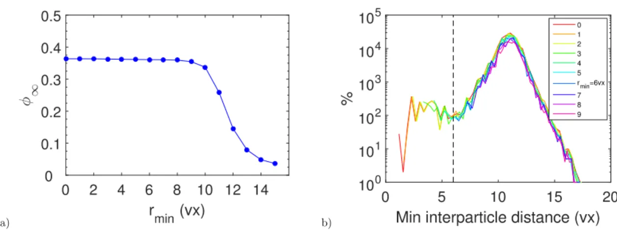
a) r ♠✁ ✥✂ ✄☎ ✵ ✷ ✹ ✻ ✽ ✶✆ ✝ ✞ ✟ ✠ ❄ ✡ ☛ ☞ ✌✍ ✎ ✏✑ ✒ ✓✔ ✕ ✖✗ ✘ ✙✚ b) ▼✛ ✜✢✣ ✤✦✧★ ✩✪✫✬ ✭ ✮✯✰✱ ✲✳ ✴✸✺ ✼✾✿ ❀❁ ❂ ❃ ❅❆ ❇ ❈ ❉ ❊ ❋ ● ❍ ■ ❏ ❑ ▲ ◆ ❖ P ◗ ❘ ❙ ❚ ❯ ❱ ❲ ❳ ❩ ❬ ❭ ❪ ❫ ❴ ❵ ❛❜ ❝ ❞❡ ❢❣ ❤ ✐ ❥
FIG. 7. a) Volume fraction φ∞(rmin) far from reference particles, computed from the number of
neighbours detected by unit volume, for different values of the threshold distance rmin (minimal
distance between two centers). b) Distribution of the interparticle distance for the identified first neighbours for all rmin ≤ 9. The visco-plastic suspension (a, b) has a solid fraction equal to
φ '36%.
value of rmin was varied excessively from 1 to 15 voxels corresponding to 0.1d and
315
1.3d, with d, the particle diameter. We see that for rmin < 9 voxel, the volume
316 317
fraction φ∞ is unchanged, and corresponds to the volume fraction of the prepared
318
particles in the suspension; for larger values of rmin, the measured volume fraction φ∞
319
decreases strongly, showing that some relevant particles are lost. Figure 7b shows the
320
distribution of inter particle distances for the identified first neighbors for all rmin ≤ 9.
321
All distributions are superimposed, but there is clearly an excess of neighbours at
322
small distances for rmin < 6, which likely corresponds to multiple centers for the same
323
particle. That is why rmin = 6 finally seems to be a good choice (Table II). Moreover
324
we checked that this choice allows to preserve the quality and quantity of the pdf.
325
Note that the values of the parameters rneigh, rmin, µmin, µmax (Tab. II) are not severely
326
chosen, ensuring no arbitrary exclusion or selection of particles and more importantly a low
327
influence of their values on our results. Finally, we do not observe any forgotten particle
328
when we systematically check some samples of 3D images.
B. Sub-voxel identification of particle centers
330
At this stage, the selected centers corresponding to exact voxel positions are identified
331
as particles. We then refine their positions at a sub-voxel resolution by using symmetry
332
properties of the absorption signal over a particle around its center (Fig. 4).
333
First, the filtered image If is linearly interpolated at the chosen sub-voxel spatial
resolu-334
tion to give Ivx(the resolution we want for the particles centers). The (tri)linear interpolation
335
lays on the following principle: the value of the voxel to interpolate (at the chosen position)
336
is taken equal to the average of the values of the (original) crossed voxels, weighted by the
337
relative partial crossed volumes.
338
Second, an algorithm searches the position (x0, y0, z0) in a range ±(δx0, δy0, δz0),
mini-339
mizing ∆I, built to quantify the asymmetry of the signal around this center, defined as:
340
∆I2 = X
∆r≤rsym
(Ivx(x0+ ∆x, y0+ ∆y, z0+ ∆z) − Ivx(x0− ∆x, y0− ∆y, z0− ∆z))2 (7)
for values of ∆r = p∆x2+ ∆y2+ ∆z2 smaller than a threshold r
sym, taken as 60% of the
341
mean diameter of particles (Tab. II).
342
A compromise between precision and computer time leads us to refine successively the
343
centers positions at 1 voxel first, then 1/2 voxel, until (1/2)n voxel, with n, the integer such
344
that the chosen spatial resolution is reached.
345
Figure 8a shows the variations of ∆I with the displacement ∆x of the center in the
x-346
direction in the range ±2 voxels, for different couple values (∆y,∆z) of the displacement of
347
the center in the y- and z-directions: there is indeed a minimum ∆Imin allowing to identify
348
the center. The same holds for ∆y and ∆z in the y- and z-directions. Figure 8b shows the
349
decrease of the minimum ∆Imin with n, the step of sub-voxel identification, what confirms
350
that the minimization and the sub-voxel refinement have still a physical sense till n = 5,
351
allowing to reach a resolution on the particles center position of (1/2)5 voxel = 0.375µm
352
' d/100. Note that n = −1 (Fig. 8b) corresponds to the case of no interpolation of the
353
images If, so that ∆Imin(n = −1) quantifies the asymmetry of the signal around the minimal
354
absorption voxel. For the results presented in this paper, a spatial resolution of 6µm ' d/20,
355
i.e. n = 1 is enough.
356
Figure 9 shows the original (non interpolated, i.e. at 1 voxel resolution, n = −1)
absorp-357
tion signal If (without unit measurement) over one particle as a function of distance from
a) ✧① ✁ ✂✄ ✲☎ ✆✝ ✵ ✶ ✷ ✞ ■ ✟ ✠ ✡ ☛☞ ✌ ✍ ✎✏ ✸ ✑ ✒✓ ✹ ✔ ✕✖ b) ♥ ✚✛ ✜ ✢ ✣ ✤ ✥ ✦ ✻ ★ ✩ ♠ ✪ ✫ ✬ ✭ ✮ ✯ ✰✱ ✳ ✴ ✼✽ ✾ ✿
FIG. 8. a) Variations of ∆I (Eq. 7) with the displacement ∆x of the center in the x-direction for the first step of sub-voxel identification n = 0. Each line corresponds to different couple values of the displacement of the center (∆y,∆z) in the y- and z-directions. b) Variations of ∆Imin with the
number of steps of sub-voxel identification n. ∆I(n = −1) quantifies the asymmetry of the signal around the minimal absorption voxel, i.e. without any interpolation of the image If . Note that
here ∆I was normalized by the number of voxels for which it has been computed to allow for a comparison at different sub-voxel resolutions
the center, for the initial center (determined from the local extrema) (Fig. 9a) and for the
359
centers refined successively with n = 0, 1, and 2 in Figure 9b, c and d respectively. We see
360
that for ∆r ≤ rsym the scattering of data (or asymmetry of the signal around its center)
361
decreases at each step of sub-voxel identification, that is quantified by ∆I. Even at 1 voxel
362
resolution (for n = 0), we already note that the center of symmetry (which is used to plot
363
Figure 9b) is not always the minimal voxel of absorption (which is used to plot Figure 9a).
364
C. Pair distribution functions
365
From particle positions within the parallel plates geometry, we are able to study how
366
particles are spatially distributed in the suspending fluid. In addition to information on the
367
structure of the suspension at the macroscopic scale from global positions of particles within
368
the geometry, we do get information on the microstructure of the suspension at the particle
369
scale from relative positions of particles (relative to each other) through the computation of
370
pair distribution functions [7].
371
The pair distribution function g(~r) is the probability of finding a particle pair separated
a) ✧r ✁✂ ✄ ✵ ✶ ✷ ✸ ✹ ✺ ✻ ✼ ✽ ✾ ☎ ✆ ■ ❢ ★✝ ✞ ✟ ✠ ✡ ☛ ☞ ✌ b) ✍✎✏✑✒ ✓ ✔ ✕ ✖ ✗ ✘ ✙ ✚ ✛ ✜ ✢ ✣ ✤ ✥ ✦ ✩ ✪✫ ✭ ✮ ✯ ✰ ✱ c) ✲✳✴✿❀ ❁ ❂ ❃ ❄ ❅ ❆ ❇ ❈ ❉ ❊ ❋ ● ❍ ❏ ❑ ▲ ▼◆ ❖ P ◗ ❘ ❙ ❚ d) ❯❱❲❳ ❨❩ ❬ ❭ ❪ ❫ ❴ ❵ ❛ ❜ ❝ ❞ ❡ ❣ ❤ ✐ ❥ ❦ ❧ ♠ ♥ ♦ ♣ q s
FIG. 9. Absorption levels (without unit measurement) of voxels over one particle and its close neighbourhood in the visco-plastic suspension at a solid fraction φ ' 40% as a function of the distance ∆r to its center, through the different steps (n = −1, 0, 1, 2 in a, b, c, d) of sub-voxel identification based on symmetrisation
by the vector ~r normalized by the mean particle density, so that the asymptotic value of g
373
for large values of ||~r|| is:
374
g(||~r|| → ∞) = 1, (8)
in the absence of macroscopic structure or long-range correlations. Equivalently, g(~r) is a
375
normalized probability of finding a (test) particle located at ~r0+ ~r with another (reference)
376
particle located at ~r0. This last definition suggests naturally how to compute g(~r): Nref
377
particles are subsequently chosen to be the reference particles; we identify the Npair test
378
particles separated by ~r from each reference particle, corresponding to the number of pairs
379
characterized by ~r in the region of interest.
380
In the following, ~r0 = (r0,θ0,z0) and ~r0 + ~r = (r,θ,z) are the cylindrical coordinates
381
(attached to the axis of the rheometer circular plates) of a reference and of a test particle
3D (-) and 2D (-+-) distances between closest neighbours in slices of different thicknesses (vx)
0 10 20 30 40 50 % 0 0.1 0.2 0.3 0.4 0.5 d/8 (3D) ∆=d (3D) 2*d (3D) d/8 (2D) ∆=d (2D) 2*d (2D)
FIG. 10. Histogram (in fraction) of the interparticle 3D (solid lines) and 2D (dashed lines with crosses) distances for the first neighbours identified in slices of different thicknesses ∆ = d/8, d and 2 ∗ d, with d, the particles’ diameter. The visco-plastic suspension has a solid fraction equal to φ ' 38%.
located in M0 and M .
383
To avoid any finite size or geometry effect on g(~r), that would introduce some bias –
384
for example underestimating the statistics in the direction of a boundary – test particles
385
shall be selected around their reference particle within an isotropic region (e.g. that does
386
not cross any boundary). To be able to study the microstructure even close to boundaries
387
(solid plates or free interfaces), we use adaptative spheres of variable radius, equal to the
388
minimal distance between the reference particle and the closest boundary, as the area where
389
searching test particles around a reference particle. In this case, we have to update the
390
number of reference particles Nref that is no more constant for all values of ~r, especially
391
for large values of ||~r||. This choice is an alternative to exclusion of regions of investigation
392
as in [14] and to a geometry-dependent correction introduced in the computation of g(~r) as
393
in [11].
394
The 3D pair distribution function g(~r) is a function of 3 scalar variables of size ∼ N3 in
395
the discretized space, with N , the number of voxels in a given direction of space. However,
396
for visualization, we generally plot the values of g(~r) taken in three orthogonal slices (data
397
of size ∼ N2). As relevant slices, we choose the cylindrical ‘planes’ attached to the axis of
398
the rheometer circular plates, as naturally suggested by the cylindrical symmetry of the
set-399
up and the flow. So, to reduce computation time, we generally compute only three 2D pair
distribution functions: gr in the orthoradial ‘plane’ (θz) normal to r (being a toroidal ring or
401
a cylinder), gθ in the radial plane (rz) normal to θ and gz in the horizontal plane (θr) normal
402
to z. So, the region where searching for test particles can be reduced to the intersection of
403
a sphere and the elementary cylindrical ‘plane’ of interest attached to the reference particle.
404
In practice, defining the elementary planes as strictly 2D slices of cylindrical coordinates
405
r = r0, θ = θ0 or z = z0 for a reference particle in M0(r0, θ0, z0) does not allow to sample
406
enough test particles and get enough statistics, so we affect elementary thicknesses to the
407
cylindrical ‘planes’. Whereas the definition of the thicknesses ∆z of horizontal planes (θr)
408
and ∆r of orthoradial ‘planes’ (θz) is obvious, the thickness of radial planes (rz) offers
409
several choices (see Appendix A). We choose the definition of:
410
∆h = r sin(θ − θ0), (9)
corresponding to a constant euclidean thickness (or minimal distance of M from the
ra-411
dial direction OM0), because it prevents a non symmetric pattern on the pair distribution
412
function gθ (see Appendix A). We checked the influence of the value ∆ of the thicknesses
413
of the planes ∆ = ∆z = ∆r = ∆h on our results. Figure 10 compares two distributions:
414
the 3D distances (real distance) and the 2D distances (projected in the slice) between first
415
neighbours of particles in an elementary cylindrical plane for different thicknesses ∆
be-416
tween d/8 and 2 ∗ d. The 3D distances are always equal or larger than d with a maximum
417
probability for d. But the 2D distances are not, because they do not represent well real 3D
418
distances in slices of thicknesses larger than d, as demonstrated by the distributions that do
419
not super-impose for ∆ > d. This leads us to choose for the thickness of elementary
cylin-420
drical ‘planes’ ∆ = d, with d the particle diameter, as a compromise between accuracy and
421
statistics. Moreover we checked that this choice allows to preserve the quality and quantity
422
of the pdfs.
423
Different choices for the characterization of the pair vector ~r ≡−−−→M0M (relative coordinates
424
between test and reference particles located in M and M0) are possible (see Appendix A).
425
Euclidean coordinates can in principle be chosen but we believe that non euclidean
coor-426
dinates, curvilinear projected along the cylindrical ‘planes’ aligned with the circular flow
427
streamlines, are more relevant to characterize the microstructure induced by a simple shear
428
flow. We choose for coordinates of the pair vector ~r = (ρ, `, ξ):
429
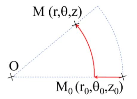
FIG. 11. Two particles M0(r0, θ0, z0) and M (r, θ, z) in the global cylindrical framework and
defini-tion of the pair vector ~r ≡ −−−→M0M characterizing their separation in curvilinear coordinates (along
circular flow lines): ~r = (ρ, `, ξ) = (r − r0, r(θ − θ0), z − z0)
as shown in Figure 11. This choice does not induce any bias in the symmetry of the pair
430
distribution functions gr, gθor gz(see Appendix A). Note that in the following, when showing
431
a 2D pdf g (gr, gθ and gz), we will use alternatively cartesian coordinates (couples among ρ,
432
` or ξ) or polar coordinates (ρ2d, φ2d) for a pair of particles in the plane of interest. In the
433
(θz), (rz) and (θr) planes, cartesian and polar coordinates are respectively related through
434
(ρ2dcos φ2d, ρ2dsin φ2d) = (`, ξ), (ρ, ξ) and (ρ, `).
435 436
Altogether, with the mean particle density (or number of particles per unit volume):
437
n0v= N/V = φ/(πd3/6), (11)
with the total number of particles N , the total volume of the suspension V , the particle
438
concentration (or solid fraction) φ, the particle diameter d, the formula for the 2D pair
439
distribution functions gr, gθ and gz in the (θz), (rz) and (θr) planes respectively (for spatial
440
resolutions δρ and δ`, δξ) are:
441
• gr(`, ξ) = Pr(`, ξ)/n0v, with Pr(`, ξ)δVr= Nrpair(` ± δ`/2, ξ ± δξ/2)/Nref,
442
• gθ(ρ, ξ) = Pθ(ρ, ξ)/n0v, with Pθ(ρ, ξ)δVθ = Nθpair(ρ ± δρ/2, ξ ± δξ/2)/Nref,
443
• gz(ρ, `) = Pz(ρ, `)/n0v, with Pz(ρ, `)δVz = Nzpair(ρ ± δρ/2, ` ± δ`/2)/Nref,
444
with Nref, the number of reference particles, and (ρ, `, ξ), the coordinates of a pair vector
445
defined in Eq. (10). While g refers to a pair distribution function, P refers to a probability
446
of finding a pair of particles and Npair to a number of pairs of particles. More precisely,
447
Npair
z (ρ±δρ/2, `±δ`/2) is the number of pairs of coordinates (ρ±δρ/2, `±δ`/2) in cylindrical
horizontal planes (θr) of thickness ∆z or equivalently the number of test particles in the
449
same horizontal plane than the reference particles (at z0), i.e. particles at z0 ± ∆z/2 ; the
450
same holds for Npair
r (` ± δ`/2, ξ ± δξ/2) and N pair
θ (ρ ± δρ/2, ξ ± δξ/2) with the thickness
451
∆r and ∆h of orthoradial plane (θz) and radial plane (rz) respectively. The elementary
452
sampling volumes (defining the spatial resolution for g in 2D) are equal to:
453
δVr = ∆rδ`δξ, δVθ = δρ∆hδξ, and δVz = δρδ`∆z. (12)
Here, the thickness of the ‘planes’ are chosen as ∆z = ∆r = ∆h = d and usually the spatial
454
resolution for pair distribution functions g is chosen as δρ = δ` = δξ = 1/2 voxel. Note
455
that these spatial averages may lead to some underestimate of peak values of g whether
456
there are large variations of g, that may lead to some discrepancies between theoretical and
457
experimental values. Finally, in three dimensions, the expression for the pdf g is:
458
g(~r ± δ~r) = Npair(~r ± δ~r)/N∞pair with N∞pair = Nrefn0vδV, (13)
N∞pair being the number of pairs separated by a vector ~r such that ||~r|| → ∞ in the sampling
459
volume δV in the space of pair vectors delimited by ~r ± δ~r.
460
In the following, the analysis of the microstructure will be generally realized, unless
spec-461
ified otherwise, far enough from the free interface and from the solid plates, to ensure not to
462
mix possible structurations near boundaries to bulk microstructure. In order to characterize
463
the microstructure for a roughly homogeneous simple shear, it has to be computed at a fixed
464
radial position R0 in the parallel plates geometry. In practice, to get a good precision of
465
the pdf, a toroidal region of sufficient thickness ∆R has to be analysed. As an example (see
466
Appendix B for details), if we want a precision ∆g = 10−2 on g(~r) and a spatial resolution
467
for the 2D pdf δV = ∆δ2 with ∆ = d = 140µm = 12vx and δ = 1vx = 12µm, for a solid
468
fraction φ = 35% (n0v = 244mm−3), we need at least 2. 104 reference particles in the region
469
of interest. This leads us to choose R0 = 0.72D/2 ± 0.12D/2, unless specified.
470
In the following, we now illustrate the potential of our technique by analyzing the
mi-471
crostructure of our suspensions near the horizontal solid plates, near the orthoradial free
472
interface, and in the bulk separately.
a) b)
FIG. 12. a) X-ray radiograph of a non sheared drop of a visco-plastic suspension at a solid fraction φ '35%. b) 3D plot of centers of all detected particle (in blue) and reference particles (in green) for the characterization of the microstructure
IV. MICROSTRUCTURE
474
A. Bulk microstructure of a non sheared visco-plastic suspension
475
First, we characterize the initial microstructure of a visco-plastic suspension poured on
476
the bottom plate of the rheometer, but before any loading and shear history. A suspension
477
is prepared by simply mixing ‘by hand’ the particles and the fluid in a cup with a spatula,
478
with the goal of achieving a mixing close to chaotic mixing. With this procedure, we aim to
479
prepare a material that is homogeneous and isotropic. It is then degased to remove possible
480
air bubbles (in a vacuum or in a centrifuge). Upon pouring, the visco-plastic suspension
481
has the shape of an irregular drop due to its yield stress (Fig. 12). Here, we analyze the
482
microstructure in a toroidal region (R0 = 0.36D/2 ± 0.30D/2 and Z0 = 2.4H ± 1.2H) inside
483
the drop far from solid surfaces and free interfaces (Fig. 12b).
484
In its initial configuration, we observe that the suspension has at first order an isotropic
485
microstructure: the pair distribution function g(~r) does not depend much on the direction
486
~r/||~r|| (Fig. 13 and 19). Figure 13 shows gr(`, ξ), gθ(ρ, ξ) and gz(ρ, `): they are roughly
487
the same in the three orthogonal 2D ‘planes’, with a circular symmetry in each 2D ‘plane’.
488
g(~r) mostly depends only on the distance ||~r||. Figure 14b shows the 1D scalar pdf g(||~r||):
489
g(||~r||) = 0 for (and only for) distances ||~r|| . d; it has a maximal value for ||~r|| ' d and a
490
second local maxima for ||~r|| ' 2d; then g tends to 1 for larger values of ||~r||.
491
Note that a closer inspection of the 2D pdfs (Fig. 13b) shows that they are not exactly
492
the same and not exactly isotropic: the averages of gr and gθ for distances ρ2d close to its
493
maxima (ρ2d = d ± d/6) as a function of φ2d (represented in a polar plot) are not perfectly
a) ✲✂ ✄ ❂❞ ☎✆ ✵ ✶ ✷ ✝✞ ✟✠ ✡ ☛ ☞ ✌ ✍ ✎ ✏ ✑ ✒ ✓✔ ✕✖ ✗ ✘ ✙ ✚ ✛ ✜ ✸ ❡ ✢ ✣ r ✤ ③ b) ❁ ✥ ❃ ✦ ✬ ✧ ★ ✻ ✩ ❄ ✪ ✫ ✯ ✰ ✱ ✳ ✴ ✹ ✺ ✼ ✽ ✿ ❅ ❆❇ ❈ ❉ ❊❋ ● ❍ ■❏ ❑ ▲ ▼ ◆ ❖ P ◗❘ ❙ ❚ ❯ ❱ ❲❳ ❨ ❩ ❬❭ ❪ ❫ ❴ ❛ ❜ ❝ ❢ ❤ ✐ ❥ ❦ ❧ ♠ ♥ ♦ ♣ q s t
FIG. 13. a) Three dimensional microstructure of a visco-plastic suspension in a non sheared con-figuration (drop) at a solid fraction φ ' 35%: 2D pair distribution functions gr(`, ξ), gθ(ρ, ξ) and
gz(ρ, `). b) Polar plots of < g(φ2d) >ρ2d=d±d/6in the three planes of interest (θz), (rz) and (θr)
a) ❣ r ✭❵❀✾✮ ❂ ❞ ✲✁ ✂✄ ✵ ✶ ✷ ☎ ✆ ✝ ✞✟ ✠✡ ☛ ☞ ✌ ✍ ✎ ✏ ✸ b) ✑ ✒ ✓ ✴✔ ✕ ✖ ✗✘ ✙ ✚ ✛✜ ✢ ✣ ✤✥ ✦ ✧ ★ ✩ ✪ ✫ ✬ ✯ ✰ ✱ ✳ ♥ ✹ ✺ ❡ ✻✼✽ ✿ ❁❃❄ ❅ ❆❇ ❈❉ ❊ ❋● ❍ ■ ❏ ❑ ▲ ▼ ◆ ❖ P ◗ ❘ ❙ ❚ ❯ ❱ ❲ ❳ ❨
FIG. 14. Numerical microstructure from a simulation of finite-size particles following a naive rule of exclusion and redistribution for a solid fraction φ ' 36%: a) 2D pair distribution function g(`, ξ) and b) 1D scalar pair distribution function g(ρ2d) super-imposed with the experimental 1D pdf for
a non sheared suspension
circular but bear a signature of a slight over-population of pairs of particles roughly aligned
495
with the gravity. This slight micro-structuration is not visible in the (θr) plane (on gz).
496
This may be attributed to vertical flows of the suspension when it is poured on the plate.
497
This almost isotropic experimental pdf is now compared to the numerical pdf obtained
498
when simulating a random distribution of finite-size particles, with a naive rule of exclusion
499
and redistribution (Fig. 14). The finite-size effect introduced here, arbitrarily governed
500
(i.e. without introducing physical forces), has to be seen as a minimal steric constraint. A
a) ❣✭ ❀ ❵ ✁✾✮ ✲✂ ✄❂ ❞ ☎✆ ✵ ✶ ✷ ✝✞ ✟✠ ✡ ☛ ☞ ✌ ✍ ✎ ✏ ✑ ✒ ✓✔ ✕✖ ✗ ✘ ✙ ✚ ✛ ✜ ✸ ❡ ③ ✢ r ✣ ✤ ⑦✉ ✥ ❴ ✳ b) ✦✧ ★ ✩✪ ✫✬✯ ✰✱ ✴ ✹ ✺ ✻✼ ✽ ✿ ❁ ❃❄ ❅❆ ❇ ❈ ❉❊ ❋ ● ❍ ■ ❏ ❑▲ ▼◆ ❖ P ◗ ❘ ❙ ❚ ❯ ❱ ❲ ❳ ❨ ❩ ❬ ❪ ❫ ❛❜
FIG. 15. Three dimensional microstructure of a visco-plastic suspension after loading and squeez-ing in a parallel plates geometry at a solid fraction φ ' 35%: 2D pair distribution functions gr(`, ξ), gθ(ρ, ξ) and gz(ρ, `) for z < 0 (a) and for z > 0 (b)
random distribution of points (representing particles of zero size) gives obviously a constant
502
pdf equal to 1 everywhere. Adding an effect of a finite size by taking away over-lapping
503
particles (separated by a distance smaller than their diameter d) and separating them by
504
their diameter d in the initial direction (and repeating this until no more particles over-lap
505
[34] ) leads to a pdf dependent on ||~r|| (Fig. 14) with the same features as the experimental
506
pdf we measure in 3D in a non sheared visco-plastic suspension, in particular local minimum
507
and secondary maximum at the same positions. The main visible difference is the width
508
and the value of the first peak of g maybe due to the difference of granulometry of the
509
particles, to the arbitrary rule of redistribution of over-lapping particles and to a specific
510
spatial distribution of particles in a non sheared suspension. Finally, the fluid does not seem
511
to have any significant impact on the microstructure during the mixing.
512
B. Bulk microstructure of a visco-plastic suspension after a continuous squeeze
513
When a suspension is loaded into a parallel plates geometry, it is first poured on the
514
bottom plate. The top plate is then translated downwards, thus squeezing the visco-plastic
515
suspension between the two plates. The flow induced by this squeeze flow is an
inhomoge-516
neous simple shear flow, which has been thoroughly described in the literature [30–32] and
517
is briefly discussed in part II D.
518
The technique developed here for the 3D characterization of microstructure allows us
a) ❣ ✸ ✭❀ ✾✮ ✁❂ ❞ ✲✂ ✄☎ ✆✝ ✵ ✶ ✷ ✞ ✟ ✠ ✡ ☛☞ ✌✍ ✎✏ ✑ ✒ ✓ ✔ ✕ ✖ ✗ ✘ ✙ ❴ ✳ b) ✚ ✛ ✜✢✣✤✥ ✦ ✧★ ✩✪ ✫✬ ✯✰ ✱ ✴ ✹ ✺ ✻ ✼ ✽ ✿❁ ❃❄ ❅❆ ❇ ❈ ❉ ❊ ❋ ● ❍ ■ ▲ ▼ ◆
FIG. 16. Pair distribution function gφ(ρ, ξ) after a squeeze flow in the shear plane for z < 0 (a)
and for z > 0 (b) a) ❁ ❣ ❃ ❞ ✬ ❂ ✻ ✭ ❄ ✷ ✁ ✮ ✵ ✂ ✸ ✄ ☎ ✆ ✝ ✞ ✟ ✠✡ ☛ ☞ ✌ ✍ ✎ ✥ ✏✑✒ ✓ ✔ ✕ ✖✗ ✘✙✚ ✾ ✛ ✜ ✶ ✢ ✣✤ ✦✧ ★ ✩ ✪ ✫✯ ✰ ✱ ✲✳ ✴ ✹ ✺ ✼✽ ✿ ❀ ❅ r ❆ ③ ⑦ ✉ ❇ ❴ ❈ b) ❉ ❊ ❋ ● ❍ ■ ❏ ❑ ▲ ▼ ◆ ❖ P ◗ ❘ ❙ ❚ ❯ ❱ ❲ ❳ ❨ ❩ ❬❭ ❪ ❫ ❵❛ ❜ ❝ ❡❢ ❤ ✐ ❥ ❦ ❧ ♠ ♥♦ ♣ q s t ✈✇ ① ② ④⑤ ⑥ ⑧ ⑨ ⑩ ❶ ❷ ❸ ❹ ❺ ❻ ❼ ❽ ❾ ❿ ➀ ➁ ➂ ➃ ➄ ➅ ➆ ➇ ➈ ➉
FIG. 17. Pair distribution functions gr, gθ and gz averaged for distances ρ2d= d ± d/6 plotted as
a function of the angle φ2d in polar coordinates after a squeeze flow for z < 0 (a) and for z > 0 (b)
for a visco-plastic suspension at a solid fraction φ ' 35%
to investigate if and how the simple shear in the (rz) plane induced by this squeeze flow
520
changes the microstructure of the suspension, initially nearly isotropic as seen above. The
521
plane in the middle of the gap, defined by z = 0, is an axis of symmetry of the flow. To take
522
into account the different sign of the shear rate (velocity gradient) in the upper and lower
523
part of the suspension, we analyse here the microstructure separately in both semi-planes
524
z < 0 and z > 0.
525
In Figures 15 and 16, we observe that an anisotropic microstructure develops in the shear
526
plane (rz) (velocity-velocity gradient plane), while it remains approximately isotropic in the
two other cylindrical planes (θz) and (θr) where the suspension does not experience any
528
shear. Contrary to the nearly isotropic microstructure observed previously in the initial
529
configuration, the pdf g(~r) is no more simply a scalar function of ||~r|| but depends both on
530
the distance ||~r|| and the direction ~r/||~r||. As in shear-induced structuration observed in the
531
literature in the case of the rotational shear of a Newtonian suspension [7, 9–14], we observe
532
here a depletion of particles in close contact (ρ2d ' d) located in the extensional area close
533
to the direction of the velocity (near the angles +15◦ and +195◦ for z < 0 and +165◦ and
534
+345◦ for z > 0). Moreover, Figure 19 shows the 1D scalar plot of g(||~r||): its maxima is
535
larger and tightens (spreads less) in comparison with the case of the non sheared suspension.
536
As previously seen, a closer inspection of the 2D pdfs (Fig. 17 and 19) by looking at
537
the averages of gr, gz and gθ for distances ρ2d close to its maxima (ρ2d = d ± d/6) as a
538
function of φ2d shows a secondary structuration in addition to the depletion of particles in
539
the (rz) plane: gr and gz exhibit an ‘hexagonal’ shape, that may be the signature of a more
540
complex flow occurring in the parallel plates than a simple shear flow as approximated in
541
the framework of lubrification when D/H is large (the flow has also a velocity component
542
aligned with the direction of translation of the bottom plate, which might not be negligible).
543
As a consequence, a suspension initially characterized by a nearly isotropic
microstruc-544
ture in 3D, develops at first an anisotropic microstructure when loaded in the parallel plates
545
geometry, even before any imposed shear history. Such impact of loading on the
microstruc-546
ture of suspension should be observed in most rheometrical devices (cone-and-plate, Couette,
547
Poiseuille, ...). If the characterization of an isotropic structure is needed, a possible
rheo-548
metrical tool is the vane in cup geometry, classically used to study gels: isotropy can be
549
achieved by chaotic mixing in the cup, and then the insertion of the vane into the cup should
550
not affect the material’s structure.
551
C. Bulk microstructure of a visco-plastic suspension after a rotational shear flow
552
After the loading of the visco-plastic suspension in the parallel plates geometry, a simple
553
shear flow in the (θz) plane is imposed thanks to the rotation of the top plate until a
554
stationary state is reached in terms of shear stress.
555
As already observed for a Newtonian suspension (numerically and experimentally) [7, 9–
556
14] and as reported in Ovarlez et al. [5] for a visco-plastic suspension, the microstructure
a) ❣✭ ❀ ❵ ✁✾✮ ✲✂ ✄ ❂❞ ☎✆ ✵ ✶ ✷ ✝✞ ✟✠ ✡ ☛ ☞ ✌ ✍ ✎ ✏ ✑ ✒ ✓✔ ✕✖ ✗ ✘ ✙ ✚ ✛ ✜ ✸ ❡ ③ ✢ r ✣ ✤ ❴ ✳ ✥ ✉ b) ❁ ✦ ❃ ✧ ✬ ★ ✩ ✻ ✪ ❄ ✫ ✯ ✰ ✱ ✴ ✹ ✺ ✼ ✽ ✿ ❅ ❆ ❇ ❈❉ ❊ ❋ ●❍ ■ ❏ ❑▲ ▼ ◆ ❖ P ◗ ❘ ❙❚ ❯ ❱ ❲ ❳ ❨ ❩ ❬ ❭ ❪❫ ❛ ❜ ❝ ❢ ❤ ✐ ❥ ❦ ❧ ♠ ♥ ♦ ♣ q s t ✈ ✇ ① ⑤ ⑥ ⑧
FIG. 18. a) Three dimensional microstructure: pair distribution functions gr(`, ξ), gθ(ρ, ξ), gz(ρ, `)
after a steady rotational shear at a shear rate ˙γ = 10−2s−1 of a visco-plastic suspension at a solid
fraction φ ' 35%. b) Pair distribution function gr, gθ and gz averaged for ρ2d= d ± d/6 plotted as
a function of the angle φ2d in polar coordinates.
becomes anisotropic in the (θz) shear plane (velocity-velocity gradient plane), while it is
ap-558
proximately isotropic in the two other ‘planes’, as shown in Figure 18 and 19: this anisotropy
559
is referred to in the literature as a fore-aft asymmetry. In 3D, it means that the positions
560
of particle pairs previously correlated in the (rz) plane due to the squeeze flow, decorrelate
561
thanks to the rotational shear and the particles reorganize themselves relatively to each
562
other, leading to some new correlations in the (θz) plane.
563
These correlations between particles develop at the scale of particle pairs in close contact,
564
leading to a depletion of particles in the extensional area, in contrast with the compressional
565
area, as well as a primary over-population roughly aligned with the direction of the flow
566
(+170◦). This anisotropy can be quantified thanks to the plots of g(φ2d) (the average of
567
g(ρ2d, φ2d) for ρ2d = d ± d/6) plotted in polar coordinates in Figure 18b: g(φ2d) has the
568
shape of a ‘butterfly’.
569
More precisely, Figure 18 shows that for distances ρ2d close to the value of the particles
570
diameter, gr has minimal values for the angles +30◦ and +210◦, corresponding to a decrease
571
of the number of pairs in the extensional stress domain; and it has maximal values for the
572
angles +170◦ and +350◦, corresponding to an increase of the number of particle pairs aligned
573
roughly with the flow. These two principal extrema can be referred to as an
extensional-574
depletion of particle pairs (for the minima of g) and a flow-alignment of particle pairs (for
575
the maxima of g). Whereas the extensional-depletion of particle pairs was already reported