HAL Id: hal-00782641
https://hal.inria.fr/hal-00782641
Submitted on 31 Jan 2013
HAL is a multi-disciplinary open access
archive for the deposit and dissemination of
sci-entific research documents, whether they are
pub-lished or not. The documents may come from
teaching and research institutions in France or
abroad, or from public or private research centers.
L’archive ouverte pluridisciplinaire HAL, est
destinée au dépôt et à la diffusion de documents
scientifiques de niveau recherche, publiés ou non,
émanant des établissements d’enseignement et de
recherche français ou étrangers, des laboratoires
publics ou privés.
Hierarchical Agglomeration and EM
Koray Kayabol, Vladimir A. Krylov, Josiane Zerubia
To cite this version:
Koray Kayabol, Vladimir A. Krylov, Josiane Zerubia. Unsupervised Classification of SAR Images
Using Hierarchical Agglomeration and EM. Computational Intelligence for Multimedia Understanding
MUSCLE 2011, Dec 2011, Pisa, Italy. pp.54-65, �10.1007/978-3-642-32436-9_5�. �hal-00782641�
using Hierarchical Agglomeration and EM
Koray Kayabol⋆, Vladimir A. Krylov⋆⋆, and Josiane Zerubia
Ariana, INRIA Sophia Antipolis Mediterranee,
2004 route des Lucioles, BP93, 06902 Sophia Antipolis Cedex, France {koray.kayabol,vladimir.krylov,josiane.zerubia}@inria.fr
http://www-sop.inria.fr/ariana/en/index.php
Abstract. We implement an unsupervised classification algorithm for high resolution Synthetic Aperture Radar (SAR) images. The founda-tion of algorithm is based on Classificafounda-tion Expectafounda-tion-Maximizafounda-tion (CEM). To get rid of two drawbacks of EM type algorithms, namely the initialization and the model order selection, we combine the CEM algorithm with the hierarchical agglomeration strategy and a model or-der selection criterion called Integrated Completed Likelihood (ICL). We exploit amplitude statistics in a Finite Mixture Model (FMM), and a Multinomial Logistic (MnL) latent class label model for a mixture den-sity to obtain spatially smooth class segments. We test our algorithm on TerraSAR-X data.
Keywords: High resolution SAR, TerraSAR-X, classification, texture, multinomial logistic, Classification EM, hierarchical agglomeration
1
Introduction
Finite Mixture Model (FMM) is a suitable statistical model to represent SAR image histogram and to perform a model based classification [1], [2]. One of the first uses of FMM in SAR image classification may be found in [3]. A combination of several different probability density functions (pdfs) into a FMM has been used in [4] for high resolution SAR images. The EM algorithm [5], [6] has been used for parameter estimation in latent variable models such as FMM. Two drawbacks of FMM based classification with EM algorithm can be sorted as 1) determination of the necessary number of class to represent the data and 2) initialization of the classes. By the term unsupervised, we refer to an initialization independent algorithm which is also able to determine the model order as in [7], [8]. There are some stochastic methods used in image segmentation like Reversible Jump Markov Chain Monte Carlo in [9], but their computational complexity is high
⋆Koray Kayabol carried out this work during the tenure of an ERCIM ”Alain
Ben-soussan” Postdoctoral Fellowship Programme.
⋆⋆ Vladimir A. Krylov carried out this work with the support of INRIA Postdoctoral
and sometimes they may reach an over segmented maps. Using the advantage of categorical random variables [10], we prefer to use an EM based algorithm called Classification EM (CEM) [11] whose computational cost is lower than both the stochastic methods and the conventional EM algorithm. In classification step, CEM uses the Winner-Take-All principle to allocate each data pixel to the related class according to the posterior probability of latent class label. After the classification step of CEM, we estimate the parameters of the class densities using only the pixels which belong to that class.
Running the EM type algorithms several times for different model orders to determine the order based on a criterion is a simple approach to reach a parsimonious solution. In [12], a combination of hierarchal agglomeration [13], EM and Bayesian Information Criterion (BIC) [14] is proposed to find the nec-essary number of classes in the mixture model. [8] performs a similar strategy with Component-wise EM [15] and Minimum Message Length (MML) criterion [16, 17]. In this study, we combine hierarchal agglomeration, CEM and ICL [18] criterion to obtain an unsupervised classification algorithm.
We use a mixture of Nakagami densities for amplitude modelling. To obtain smooth and segmented class label maps, a post-processing can be applied to roughly classified class labels, but a Bayesian approach allows to include smooth-ing constraints to classification problems. We assume that each latent class label is a categorical random variable which is a special version of the multinomial random variable where each pixel belongs to only one class [1]. We introduce a spatial interaction within each binary map adopting multinomial logistic model [19], [10] to obtain a smooth segmentation map.
In Section 2 and 3, the MnL mixture model and CEM algorithm are given. We give the details of the agglomeration based unsupervised classification algorithm in Section 4. The simulation results are shown in Section 5. Section 6 presents the conclusion and future work.
2
Multinomial Logistic Mixture of Amplitude based
Densities
We assume that the observed amplitude at the nth pixel, sn ∈ R+, where n ∈
R = {1, 2, . . . , N } represents the lexicographically ordered pixel index, is free from any noise and instrumental degradation. Every pixel in the image has a latent class label. Denoting K the number of classes, we encode the class label as a K dimensional categorical vector zn whose elements zn,k, k ∈ {1, 2, . . . , K}
have the following properties: 1) zn,k ∈ {0, 1} and 2) PKk=1zn,k = 1. We may
write the probability of sn as the marginalization of the joint probability of
p(sn, zn|Θ, πn) = p(sn|zn, Θ)p(zn|πn), [1], as p(sn|Θ, πn) = X zn p(sn|zn, Θ)p(zn|πn) =X zn K Y k=1 [p(sn|θk)πn,k]zn,k (1)
where πn,k = p(zn,k= 1) represent the mixture proportions, πn = [πn,1, . . . , πn,K],
θk is the parameter of the class density and Θ = {θ1, . . . , θK} is the set of the
parameters. If zn is a categorical random vector and the mixture proportions
are spatially invariant, (1) is reduced to classical FMM as follow:
p(sn|Θ) = K
X
k=1
p(sn|θk)πk (2)
We prefer to use the notation in (1) to show the contribution of the multinomial density of class label, p(zn), into finite mixture model more explicitly. We give
the details of the class and the mixture densities in the following two sections.
2.1 Class Amplitude Densities
Our aim is to use the amplitude statistics to classify the SAR images. For this purpose, we model the class amplitudes using Nakagami density, which is a basic theoretical multi-look amplitude model for SAR images [2]. We express the Nakagami density with parameters µk and νk as in [2], [10] as
pA(sn|µk, νk) = 2 Γ(νk) µ νk µk ¶νk s2νk−1 n e −νk s2n µk . (3) We denote θk = {µk, νk}.
2.2 Mixture Density - Class Prior
The prior density p(zn,k|πn,k) of the categorical random variable is naturally
an iid multinomial density, but we are not able to obtain a smooth class label map if we use an iid multinomial. We need to use a density which models the spatial smoothness of the class labels as well. We use a contrast function which emphasizes the high probabilities while attenuating the low ones, namely Logis-tic function [19]. The logisLogis-tic function allows us to make an easier decision by discriminating the probabilities closed to each other. In this model, We are also able to introduce spatial interactions of the categorical random field by defining a binary spatial auto-regression model. Our MnL density for the problem at hand is written as p(zn|Z∂n, η) = K Y k=1 Ã exp(ηvk(zn,k)) PK j=1exp(ηvj(zn,j)) !zn,k (4) where vk(zn,k) = 1 + X m∈M(n) zm,k. (5)
and Z∂n = {zm : m ∈ M(n), m 6= n} is the set which contains the neighbors
of zn in a window M(n) defined around n. The function vk(zn,k) returns the
number of labels which belong to class k in the given window. The mixture density in (4) is spatially-varying with given function vk(zn,k) in (5).
3
Classification EM Algorithm
Since our purpose is to cluster the observed image pixels by maximizing the marginal likelihood given in (1), we suggest to use EM type algorithm to deal with the summation. The EM log-likelihood function is written as
QEM(Θ|Θt−1) = N X n=1 K X k=1 zn,klog{p(sn|θk)πn,k}p(zn,k|sn, Z∂n, Θt−1) (6)
where we include the parameter η to parameter set Θ = {θ1, . . . , θK, η}.
If we used the exact EM algorithm to find the maximum of Q(Θ|Θt−1) with
respect to Θ, we would need to maximize the parameters for each class given the expected value of the class labels. Instead of this, we use the advantage of working with categorical random variables and resort to Classification EM algorithm [11]. After classification step, we can partition the pixel domain R into K non-overlapped regions such that R =SK
k=1Rk and RkT Rl= 0, k 6= l
and consequently, we may write the classification log-likelihood function as
QCEM(Θ|Θt−1) = K X k=1 X m∈Rk log{p(sm|θk)πm,k}p(zm,k|sm, Z∂m, Θt−1) (7)
The CEM algorithm incorporates a classification step between the E-step and the M-step which performs a simple Maximum-a-Posteriori (MAP) estimation to find the highest probability class label. Since the posterior of the class label p(zn,k|sn, Z∂n, Θt−1) is a discrete probability density function of a finite number
of classes, we can perform the MAP estimation by choosing the maximum class probability. We summarize the CEM algorithm for our problem as follows:
E-step: For k = 1, . . . , K and n = 1, . . . , N , calculate the posterior proba-bilities p(zn,k|sn, Z∂n, Θt−1) = p(sn|θt−1k ) exp(ηt−1v k(zn,k)) PK j=1exp(ηt−1vj(zn,j)) (8)
given the previously estimated parameter set Θt−1.
C-step: For n = 1, . . . , N , classify the nth pixel into class j as zn,j = 1 by
choosing j which maximizes the posterior p(zn,k|sn, Z∂n, Θt−1) over k = 1, . . . , K
as
j= arg max
k p(zn,k|sn, Z∂n, Θ
t−1) (9)
M-step: To find a Bayesian estimate, maximize the classification log-likelihood in (7) with respect to Θ as
Θt−1= arg max
Θ QCEM(Θ|Θ
t−1) (10)
To maximize this function, we alternate among the variables µk, νk and η.
We use the following methods to update the parameters: analytical solution of the first derivative for µk, zero finding of the first derivative for νk and
4
Unsupervised Classification Algorithm
In this section, we present the details of the unsupervised classification algorithm. Our strategy follows the same general philosophy as the one proposed in [13] and developed for mixture model in [8, 12]. We start the CEM algorithm with a large number of classes, K = Kmax, and then we reduce the number of classes
to K ← K − 1 by merging the weakest class in probability to the one that is most similar to it with respect to a distance measure. The weakest class may be found using the average probabilities of each class as
kweak= arg min k 1 Nk X n∈Rk p(zn,k|sn, Z∂n, Θt−1) (11)
Kullback-Leibler (KL) type divergence criterions are used in hierarchical tex-ture segmentation for region merging [20]. We use a symmetric KL type distance measure called Jensen-Shannon divergence [21] which is defined between two probability density functions, i.e. pkweak and pk, k 6= kweak, as
DJ S(k) =
1
2DKL(pkweak||q) +
1
2DKL(pk||q) (12) where q = 0.5pkweak + 0.5pk and
DKL(p||q) =
X
k
p(k) logp(k)
q(k) (13)
We find the closest class to kweak as
l= arg min
k DJ S(k) (14)
and merge them to constitute a new class Rl← RlS Rkweak.
We repeat this procedure until we reach the predefined minimum number of classes Kmin. We determine the necessary number of classes by observing the
ICL criterion explained in Section 4.3. The details of the initialization and the stopping criterion of the algorithm are presented in Section 4.1 and 4.2. The summary of the algorithm can be found in Table 1.
4.1 Initialization
The algorithm can be initialized by determining the class areas manually in case that there are a few number of classes. We suggest to use an initialization strategy for completely unsupervised classification. It removes the user intervention from the algorithm and enables to use the algorithm in case of large number of classes. First, we run the CEM algorithm for one global class. Using the cumulative distribution of the fitted Nakagami density g = FA(sn|µ0, ν0) where g ∈ [0, 1]
and dividing [0, 1] into K equal bins, we can find our initial class parameters as µk = FA−1(gk|µ0, ν0), k = 1, . . . , K where gk’s are the centers of the bins.
We initialize the other parameters using the estimated parameters of the global class.
Table 1. Unsupervised CEM algorithm for classification of amplitude based mixture model.
Initialize the classes defined in Section 4.1 for K = Kmax.
While K≥ Kmin, do
While the condition in (15) is false, do E-step: Calculate the posteriors in (8) C-step: Classify the pixels regarding to (9) M-step: Estimate the parameters of amplitude and texture densities as (10)
Find the weakest class using (11)
Find the most similar class to the weakest class using (12-14)
Merge these two classes Rl← RlS Rkweak
K← K − 1
4.2 Stopping Criterion
We observe the normalized and weighted absolute difference between sequential values of parameter set θkto decide the convergence of the algorithm. We assume
that the algorithm has converged, if the following expression is satisfied:
K X k=1 Nk|θtk− θ t−1 k | N|θt−1k | ≤ 10 −3 (15)
4.3 Choosing the Number of Classes
Although the SAR images which we used have a small number of classes, we validate our assumption on number of classes using the Integrated Completed Likelihood (ICL) [18]. Even though BIC is the most used and the most practical criterion for large data sets, we prefer to use ICL because it is developed specif-ically for classification likelihood problem, [18], and we have obtained better results than BIC in the determination of the number of classes. In our problem, the ICL criterion may be written as
ICL(K) = N X n=1 K X k=1 log{p(sn|ˆθk)ˆzn,kp(ˆzn,k| ˆZ∂n,η)} −ˆ 1 2dKlog N (16) where dK is the number of free parameters. In our case, it is dK = 12 ∗ K + 1.
ˆ
zn,k is the maximum a posterior estimate of zn,k found in C-step.
We also use the BIC criterion for comparison. It can be written as
BIC(K) = N X n=1 log à K X k=1 p(sn|ˆθk)p(zn,k|Z∂n,η)ˆ ! −1 2dKlog N (17)
5
Simulation Results
This section presents the high resolution SAR image classification results of the proposed method called AML-CEM (Amplitude density mixtures of MnL with CEM), compared to the corresponding results obtained with other methods which are DSEM-MRF [22] and K-MnL. We have also tested supervised version of AML-CEM [10] where training and testing sets are determined by selecting some spatially disjoint class regions in the image, and we run the algorithm twice for training and testing. The sizes of the windows for texture and label models are selected to be 3×3 and 13×13 respectively by trial and error. We initialize the algorithm as described in Section 4.1 and estimate all the parameters along the iterations.
The K-MnL method is the sequential combination of K-means clustering for classification and Multinomial Logistic label model for segmentation to obtain a fairer comparison with the K-means clustering since K-means does not provide any segmented map. The weak point of the K-means algorithm is that it does not converge to the same solution every time, since it starts with random seed. Therefore, we run the K-MnL method 20 times and select the best result among them.
We tested the algorithms on the following TerraSAR-X image:
– TSX1: 1200 × 1000 pixels, HH polarized TerraSAR-X Stripmap (6.5 m ground resolution) 2.66-look geocorrected image which is acquired over San-chagang, China (see Fig. 1(a)). c°Infoterra.
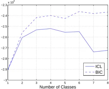
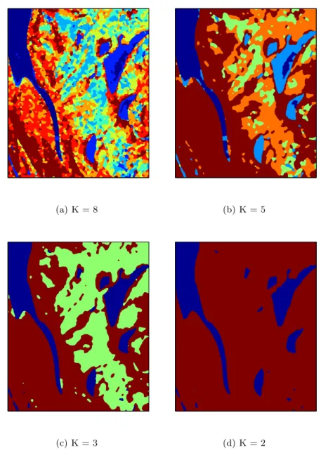
For TSX1 image in Fig.1(a), the full ground-truth map has been generated manually. Fig.1 shows the classification results where the red colored regions indicate the misclassified parts according to 3-classes ground-truth map. We can see the plotted ICL and BIC values with respect to number of classes in Fig. 2. The variations in the ICL and BIC plots are slowed down after 3. ICL reaches its maximum value at 4. Since the difference between the values at 3 and 4 is very small and our aim is to find the minimum number of classes, we may say that the mixture model with 3 number of classes is almost enough to represent this data set. Fig. 3 shows several classification maps found with different numbers of classes. From this figure, we can see the evolution of the class maps along the agglomeration based algorithm. The numerical accuracy results are given in Table 2 for 3-classes. The supervised AML-CEM gives the best result over all. In supervised methods, the accuracy results of K-MnL is a bit better than those of unsupervised AML-CEM, but K-MnL is able to provide these results in case of a given number of classes. Due to this, we may call K-MnL as a semi-supervised method.
The simulations were performed on MATLAB platform on a PC with Intel Xeon, Core 8, 2.40 GHz CPU. The total 57 iterations are performed in 5.07 minutes for K = 1, . . . , 8 to plot the graphic in Fig. 2 and the total number of the processed pixels are about 1.2 millions.
(a) TSX1 image (b) K-MnL classification
(c) Supervised classification (d) Unsupervised classification Fig. 1. (a) TSX1 image, (b), (c) and (d) classification maps obtained by K-MnL, supervised and unsupervised ATML-CEM methods. Dark blue, light blue, yellow and red colors represent water, wet soil, dry soil and misclassified areas, respectively.
1 2 3 4 5 6 7 8 −3 −2.9 −2.8 −2.7 −2.6 −2.5 −2.4 −2.3x 10 6 Number of Classes ICL BIC
Fig. 2.ICL and BIC values of the classified TSX1 image for several numbers of sources (from 1 to 8).
Table 2.Accuracy of the classification of TSX1 image in water, wet soil and dry soil areas and average.
water wet soil dry soil average DSEM-MRF (Sup.) 90.00 69.93 91.28 83.74
AML-CEM (Sup.) 88.98 71.21 93.06 84.42 K-MnL (Semi-sup.) 89.71 86.13 72.42 82.92 AML-CEM (Unsup.) 88.24 62.99 96.39 82.54
(a) K = 8 (b) K = 5
(c) K = 3 (d) K = 2
Fig. 3.Classification maps of TSX1 image obtained with unsupervised ATML-CEM method for different numbers of classes K = {2,3,5,8}.
6
Conclusion and Future Work
Using an agglomerative type unsupervised classification method, we eliminate the negative effect of the latent class label initialization. According to our experi-ments, the larger number of classes, we start the algorithm with, the more initial value independent results, we obtain. Consequently, the computational cost is increased as a by-product. The classification performance may be increased by including additional features as texture or polarization.
Acknowledgments. The authors would like to thank Aur´elie Voisin (Ariana INRIA, France) for interesting discussions and Astrium-Infoterra GmbH for pro-viding the TerraSAR-X image.
References
1. Titterington, D., Smith, A., Makov, A.: Statistical Analysis of Finite Mixture Dis-ributions. 3rd ed. John Wiley & Sons, Chichester (U.K.) (1992)
2. Oliver, C., Quegan, S.: Understanding Synthetic Aperture Radar Images. 3rd ed. Artech House, Norwood (1998)
3. Masson, P., Pieczynski, W.: SEM Algorithm and Unsupervised Statistical Segmen-tation of Satellite Images. IEEE Trans. Geosci. Remote Sens. 31(3), 618–633 (1993) 4. Krylov, V.A., Moser, G., Serpico, S.B., Zerubia, J.: Supervised Enhanced Dictionary-Based SAR Amplitude Distribution Estimation and Its Validation With Very High-Resolution Data. IEEE Geosci. Remote Sens. Lett., 8(1), 148–152 (2011) 5. Dempster, A.P., Laird, N.M., Rubin, D.B.: Maximum Likelihood from Incomplete
Data via the EM Algorithm. J. R. Statist. Soc. B. 39, 1-22 (1977)
6. Redner, R.A., Walker, H.F.: Mixture Densities, Maximum Likelihood and the EM Algorithm. SIAM Review, 26(2), 195–239 (1984)
7. Palubinskas, G., Descombes, X., Kruggel, F.: An Unsupervised Clustering Method using the Entropy Minimization. In: Int. Conf. Pattern Recognition, ICPR’98, 1816– 1818 (1998)
8. Figueiredo, M.A.T., Jain, A.K.: Unsupervised Learning of Finite Mixture Models. IEEE Trans. on Pattern Anal. Machine Intell. 24(3), 381–396 (2002)
9. Wilson, S.P., Zerubia, J.: Segmentation of Textured Satellite and Aerial Images by Bayesian Inference and Markov Random Fields. Res. Rep. RR-4336, INRIA, France, (2001)
10. Kayabol, K., Voisin, A., Zerubia, J.: SAR Image Classification with Non-stationary Multinomial Logistic Mixture of Amplitude and Texture Densities. In: Int. Conf. Image Process. ICIP’11, accepted, (2011)
11. Celeux, G., Govaert, G.: A Classification EM Algorithm for Clustering and Two Stochastic Versions. Comput. Statist. Data Anal. 14, 315–332 (1992)
12. Fraley, C., Raftery, A.: Model-based Clustering, Discriminant Analysis, and Den-sity Estimation. J. Am. Statistical Assoc. 97(458), 611–631 (2002)
13. Ward, J.H.: Hierarchical groupings to optimize an objective function. J. Am. Sta-tistical Assoc. 58(301), 236–244 (1963)
14. Schwarz, G.: Estimating the Dimension of a Model. Annals of Statistics 6, 461–464 (1978)
15. Celeux, G., Chretien, S., Forbes, F., Mkhadri, A.: A Component-wise EM Algo-rithm for Mixtures. Res. Rep. RR-3746, INRIA, France (1999)
16. Wallace, C.S., Boulton, D.M.: An Information Measure for Classification. Comp. J., 11, 185–194 (1968)
17. Wallace, C.S., Freeman, P.R.: Estimation and Inference by Compact Coding. J. R. Statist. Soc. B, 49(3), 240–265 (1987)
18. Biernacki, C., Celeux, G., Govaert, G.: Assessing a Mixture Model for Clustering with the Integrated Completed Likelihood. IEEE Trans. on Pattern Anal. Machine Intell. 22(7), 719–725, (2000)
19. Krishnapuram, B., Carin, L., Figueiredo, M.A.T., Hartemink, A.J.: Sparse Multi-nomial Logistic Regression: Fast Algorithms and Generalization Bounds. IEEE Trans. on Pattern Anal. Machine Intell. 27(6), 957–968 (2005)
20. Scarpa, G., Gaetano, R., Haindl, M., Zerubia, J.: Hierarchical Multiple Markov Chain Model for Unsupervised Texture Segmentation. IEEE Trans. Image Process. 18(8), 1830–1843 (2009)
21. Lin, J.: Divergence Measures Based on the Shannon Entropy. IEEE Trans. Inform. Theory 37(1), 145–151 (1991)
22. Krylov, V.A., Moser, G., Serpico, S.B., Zerubia, J.: Supervised High-Resolution Dual-Polarization SAR Image Classification by Finite Mixtures and Copulas. IEEE J. Sel. Top. Signal Process., 5(3), 554–566 (2011)