HAL Id: hal-00781447
https://hal.inria.fr/hal-00781447v4
Submitted on 3 Aug 2015HAL is a multi-disciplinary open access
archive for the deposit and dissemination of sci-entific research documents, whether they are pub-lished or not. The documents may come from teaching and research institutions in France or
L’archive ouverte pluridisciplinaire HAL, est destinée au dépôt et à la diffusion de documents scientifiques de niveau recherche, publiés ou non, émanant des établissements d’enseignement et de recherche français ou étrangers, des laboratoires
The snapping out Brownian motion
Antoine Lejay
To cite this version:
Antoine Lejay. The snapping out Brownian motion. Annals of Applied Probability, Institute of Mathematical Statistics (IMS), 2016, 26 (3), pp.1727-1742. �10.1214/15-AAP1131�. �hal-00781447v4�
The snapping out Brownian motion
Antoine Lejay
1,2,3,4,5August 3, 2015
Abstract
We give a probabilistic representation of a one-dimensional diffusion equation where the solution is discontinuous at0 with a jump proportional to its flux. This kind of interface condition is usually seen as a semi-permeable barrier. For this, we use a process called here the snapping out Brownian motion, whose properties are studied. As this construction is motivated by applications, for example in brain imaging or in chemistry, a simulation scheme is also provided.
Keywords: Interface condition, elastic Brownian motion, semi-permeable barrier, thin layer, piecing out a Markov process.
1. Introduction
Many diffusion phenomena have to deal with interface conditions. Let 𝐷 be a diffusivity coefficient which is smooth away from a regular surface 𝑆, but presents some discontinuity there. In this case, the solution to the diffusion equation
𝜕𝑡𝑢(𝑡, 𝑥) =
1
2∇(𝐷(𝑥)∇𝑢(𝑡, 𝑥)) = 0 with 𝑢(0, 𝑥) = 𝑓(𝑥) (1) has to be understood as a weak solution. However, 𝑢 is smooth away from 𝑆 and satisfies
𝑢(𝑡, 𝑥+) = 𝑢(𝑡, 𝑥−) and 𝐷(𝑥+)𝑛+(𝑥)· ∇𝑢(𝑡, 𝑥+) = 𝐷(𝑥−)𝑛−(𝑥)· ∇𝑢(𝑡, 𝑥−), (2)
1Université de Lorraine, Institut Élie Cartan de Lorraine, UMR 7502, Vandœuvre-lès-Nancy,
F-54500, France
2CNRS, Institut Élie Cartan de Lorraine, UMR 7502, Vandœuvre-lès-Nancy, F-54500, France 3Inria, TOSCA, Villers-lès-Nancy, F-54600, France
4Contact: IECL, BP 70238, F-54506 Vandœuvre-lès-Nancy CEDEX, France. Email:
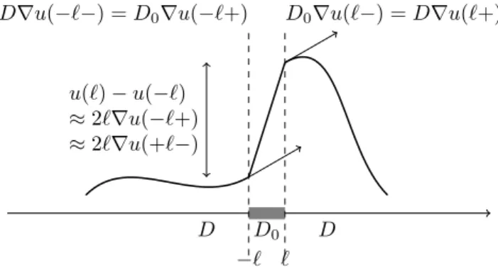
D0 D D −` ` u(`)− u(−`) ≈ 2`∇u(−`+) ≈ 2`∇u(+`−)
D∇u(−`−) = D0∇u(−`+) D0∇u(`−) = D∇u(`+)
Figure 1: The thin layer problem.
for 𝑥 ∈ 𝑆, when 𝑆 is assumed to separate locally R𝑑 into a “+” and a “-” part and where 𝑛± is a vector normal to 𝑆 at 𝑥 pointing to the “±” side. The second condition is called the continuity of the flux.
Now, let us assume that 𝐷 takes scalar values, and is constant away from a thin layer of width 2ℓ enclosed between two parallel surfaces 𝑆+ and 𝑆−. When the
width ℓ of the layer tends to 0, 𝑆+ and 𝑆− merge into a a single interface located
on a surface 𝑆.
When the diffusivity 𝐷0 decreases to 0 with ℓ and 𝐷0/ℓ → 𝜆 > 0, then the
solution to (1) converges to a function 𝑣 satisfying (1) away from 𝑆 with the interface condition for 𝑥∈ 𝑆:
∇𝑣(𝑡, 𝑥+) = ∇𝑣(𝑡, 𝑥−) and 𝜆
2(𝑣(𝑡, 𝑥+)− 𝑣(𝑡, 𝑥−)) = 𝐷(𝑥±)∇𝑣(𝑡, 𝑥±). (3) The solution has a continuous flux on 𝑆 but is discontinuous on 𝑆 (See for example [33, Chap. 13]). A heuristic explanation is given Figure 1.
If 𝐷 is smooth on R𝑑, it is well known that
𝑢(𝑡, 𝑥) = E𝑥[𝑓 (𝑋𝑡)], (4)
where 𝑋 is the diffusion process generated by 12∇(𝐷∇) which is solution under P𝑥
to the stochastic differential equation (SDE) 𝑋𝑡= 𝑥 + ∫︁ 𝑡 0 𝜎(𝑋𝑠) d𝐵𝑡+ ∫︁ 𝑡 0 1 2 𝑑 ∑︁ 𝑖=1 𝐷𝑖,· 𝜕𝑥𝑖 (𝑋𝑠) d𝑠 with 𝜎𝜎T = 𝐷 (5)
for a Brownian motion 𝐵.
When 𝐷 presents some discontinuities, (5) has no longer a meaning. However, a Feller processes (𝑋, (ℱ𝑡)𝑡≥0, (P𝑥)𝑥∈R) is associated to 12∇(𝐷∇·) for which (4) holds.
In particular, the marginal distributions 𝑋𝑡 have a density 𝑝(𝑡, 𝑥,·) under P𝑥, where
Let us now assume that the dimension of the space is equal to 1 and that 𝐷 is discontinuous at some separated points {𝑥𝑖} with left and right limit there, and
smooth elsewhere. The process 𝑋 is solution to a SDE with local time. The Itô-Tanaka formula is the key tool to manipulate it, and several simulation algorithms have been proposed (See the references in [26] for example). The process called the Skew Brownian motion is the main tool for this construction [24, 25].
Coming back to the thin layer problem, we assume that 𝐷 is constant and equal to 𝐷1 on (−∞, −ℓ) and (ℓ, ∞), and to 𝐷0 on (−ℓ, ℓ). The associated stochastic
process is solution to 𝑋𝑡= 𝑥 + ∫︁ 𝑡 0 √︀ 𝐷(𝑋𝑠) d𝐵𝑠+ 𝐷1− 𝐷0 𝐷1+ 𝐷0 𝐿ℓ𝑡(𝑋) + 𝐷0− 𝐷1 𝐷1+ 𝐷0 𝐿−ℓ𝑡 (𝑋),
where 𝐿±ℓ𝑡 (𝑋) is the local time of 𝑋 at ±ℓ [25].
Letting 𝐷0/ℓ converging to 2𝜅 with ℓ→ 0, one may expect that 𝑋 converges
in distribution to a stochastic process 𝑌 such that the solution to (1) with the interface condition (3) is given by 𝑣(𝑡, 𝑥) = E𝑥[𝑓 (𝑌𝑡)].
The article then aims at constructing and giving several properties related to the process 𝑌 which we call a snapping out Brownian motion (SNOB). This process is Feller on G = (−∞, 0−] ∪ [0+, +∞) but not on R. The intervals in the definition of G are disjoint so that 0 corresponds either to 0+ or 0− seen as distinct points. The behavior of this process is the following: Assume that its starting point is 𝑥≥ 0. It behaves as a positively reflected Brownian motion until its local time is greater than an independent exponential random variable of parameter 2𝜅. Then its decides its sign with probability 1/2 and starts afresh as a new reflected Brownian motion, until its local time is greater than a new exponential random variable, and so on... Using the properties of the exponential random variable, it is equivalent to assert that the particle changes its sign when its local time is greater than an exponential random variable with parameter 𝜅, and behaves like a positively or negatively reflected Brownian motion between these switching times.
Its name is justified by the following fact: As the time at which the particle possibly changes it signs is the same as for the elastic Brownian motion [10, 15, 18, 19] (also called the partially reflected Brownian motion), it could also be seen as some elastic Brownian motion which is reborn once killed.
The elastic Brownian motion, also called a partially reflected Brownian motion, is associated to the Robin boundary condition and has then many applications [8, 15, 35]. This process is the “basic brick” for constructing the SNOB.
The behavior of the SNOB justifies also the old heuristic that the interface condition (3) corresponds to a semi-permeable barrier, which arises for example in diffusion Magnetic Resonance Imaging [11] or in chemistry [1, 8]. The interface condition (3) is different from (2), to which is associated a Skew Brownian motion
and where the particle crosses the interface when it reaches it, and which corresponds to a permeable barrier (See references in [24, 26]).
Here, we work under the condition of a single interface at 0. In short time, it is sufficient to describe the behavior of the process even in a more complex media, since other interface or boundary conditions far enough have “exponentially small” influence on the distribution of the process. This is sufficient for simulation purposes, where particles positions are represented by the stochastic process and move according to its dynamic.
Using similar computations, one may generalize our work to the case where 𝐷(𝑥) = 𝐷+ if 𝑥≥ 0, 𝐷− if 𝑥
≤ 0 and an interface condition
∇𝑢(𝑡, 0+) = 𝛽∇𝑢(𝑡, 0−) and 𝜆𝑢(𝑡, 0+) − 𝜇𝑢(𝑡, 𝑥−) = ∇𝑢(𝑡, 𝑥+)
with 𝜆, 𝜇 > 0. Diffusions on graphs specified by a condition at each vertex could also be considered, which could be of interest in several applications. This process has been described without proof by R. Bobrowski in [6], which have studied its limit behavior when the diffusion coefficients increase.
Although the SNOB may be seen as a diffusion on a graph, it is not a diffusion on a metric graph, where the edges are joined by vertices. Such diffusions have been classified by M. Freidlin and A. Wentzell in [12, 13]. The conditions that are required at the vertices of the graphs are some extension of the possible boundary conditions for a Markov process studied by W. Feller [10]. See also [21] for example for the related problem of pasting diffusions1.
Our interface condition does not fall in these categories. Our process is best thought as a kind of random evolution process which switches back and forth randomly among a collection of processes (See e.g. [16, 34]).
Outline. In Sections 2 and 3, we present quickly the main results related to the Elastic Brownian motions and the piecing out procedure. The SNOB is constructed in Section 4 through its resolvent. In Section 5, we show the relationship between the SNOB and the thin layer problem. Finally, in Section 6, we show how to simulate this process.
2. Elastic Brownian motion
Let (𝑅𝑡)𝑡≥0 a reflected Brownian motion, and denote by (𝐿𝑡)𝑡≥0 its symmetric local
time at 0. We add a cemetery point † to R+. For a constant 𝜅 > 0, we consider an
exponential random variable 𝜉 with parameter 𝜅 independent from 𝐵. Set 𝑍𝑡 =
{︃
𝑅𝑡 if 𝐿𝑡≤ 𝜉,
† if 𝐿𝑡> 𝜉.
1The article [32] defines a notion of semipermeable membrane which is different from ours,
Thanks to the properties of the local time, this process called the elastic Brownian motion (EBM), is still a strong Markov process. It semi-group is
𝑃𝑡e𝑓 (𝑥) = E𝑥[exp(−𝜅𝐿𝑡)𝑓 (𝑋𝑡)]
for 𝑓 in the set𝒞0(R+, R) of continuous functions that vanishes at infinity. Closed
form expressions of the density transition function are given in [14, 35].
Let k be the time at which the EBM is killed, which means k = inf{𝑡 > 0 | 𝐿𝑡≥ 𝜉}.
This is a stopping time. Since the local time increases only on the closure of 𝒵 = {𝑡 > 0 | 𝑋𝑡 = 0}, it holds that 𝑍k = 0 almost surely. Using standard
computations in the inverse of the local time of the Brownian motion, 𝜓(𝑥, 𝛼) = E𝑥[exp(−𝛼k)] = 𝜅 √ 2𝛼 + 𝜅exp(− √ 2𝛼𝑥). (6)
Using the Itô formula, it is easily shown that 𝑢(𝑡, 𝑥) = 𝑃e
𝑡𝑓 (𝑥) is solution to
the heat equation with Robin (or third kind) boundary condition [3, 15, 31] {︃𝜕𝑢(𝑡,𝑥) 𝜕𝑡 = 1 2△𝑢(𝑡, 𝑥) on (0, +∞) 2, 𝜕𝑢(𝑡,0) 𝜕𝑥 = 𝜅𝑢(𝑡, 0).
For a Markov process 𝑋, let us recall that its resolvent (𝐺𝛼)𝛼>0 is a family
of operators defined by 𝐺𝛼𝑓 (𝑥) = E𝑥 [︁ ∫︀+∞ 0 𝑒 −𝛼𝑠𝑓 (𝑋 𝑠) d𝑠 ]︁
for any 𝑓 ∈ 𝒞0 and any
𝛼 > 0. It has a density 𝑔𝛼 when 𝐺𝛼𝑓 (𝑥) =∫︀ 𝑔𝛼(𝑥, 𝑦)𝑓 (𝑦) d𝑦.
Using standard computations on the Green functions, the density 𝑔e
𝛼(𝑥, 𝑦) of
the resolvent of the EBM is for 𝑥, 𝑦 ≥ 0,
𝑔e𝛼(𝑥, 𝑦) = √1 2𝛼 {︃√2𝛼−𝜅 √ 2𝛼+𝜅𝑒 −√2𝛼(𝑦+𝑥)+ 𝑒−√2𝛼(𝑥−𝑦) for 𝑦 ∈ [0, 𝑥], 𝑒 √ 2𝛼(𝑥−𝑦)+ √√2𝛼−𝜅 2𝛼+𝜅𝑒 −√2𝛼(𝑥+𝑦) for 𝑦 ≥ 𝑥.
We extend the EBM to a process on G by symmetry, so that its resolvent becomes 𝐺e𝛼𝑓 (𝑥) := E𝑥 [︂∫︁ k 0 𝑒−𝛼𝑠𝑓 (𝑋𝑠) d𝑠 ]︂ = ∫︁ +∞ 0 𝑔𝛼e(|𝑥|, 𝑦)𝑓(sgn(𝑥)𝑦) d𝑦 (7) for 𝑥 ∈ G. This process evolves either on R− or R+ but never crosses 0 and is
naturally identified with a process on G. 3. Piecing out Markov processes
The procedure of piecing out is a way to construct a Markov process from a killed one. We present in this Section a result due to N. Ikeda, M. Nagasawa and S. Watanabe [17] (Similar considerations are given in [29]).
On a probability space (Ω,ℱ, P) and a state space S, let ((𝑋𝑡)𝑡≥0, (ℱ𝑡)𝑡≥0, (P𝑥)𝑥∈S)
be a right continuous strong Markov process living in the extended state space S†= S∪ {†} with a death point †. The lifetime of 𝑋 is denoted by k.
The shift operator associated to 𝑋 is denoted by (𝜃𝑡)𝑡≥0.
We also consider a family 𝜇 defined on Ω× S† such that 𝜇(𝜔,·) is a probability measure on S† and for any fixed Borel subset 𝐴, 𝜇(·, 𝐴) is 𝜎(𝑋𝑡, 𝑡≥ 0)-measurable.
We assume additionally that 𝜇(𝜔, d𝑦) = 𝛿†(d𝑦) when k(𝜔) = 0 and
P𝑥[𝜇(𝜔, d𝑦) = 𝜇(𝜃t(𝜔)𝜔, d𝑦), t(𝜔) < k(𝜔)] = P𝑥[t < k]
for any stopping time t. The family 𝜇, called an instantaneous distribution, describes the way the process is reborn once killed.
Let ̂︀Ω be the product of an infinite, countable, number of copies of Ω× S†. We define 𝑋 on ̂︀Ω by 𝑋𝑡(𝜔) =̂︀ ⎧ ⎪ ⎪ ⎪ ⎪ ⎪ ⎪ ⎪ ⎪ ⎨ ⎪ ⎪ ⎪ ⎪ ⎪ ⎪ ⎪ ⎪ ⎩ 𝑥𝑡(𝜔1) if 𝑡 ∈ [0, k(𝜔1)), 𝑦1 if 𝑡 = k(𝜔1), 𝑥𝑡−k(𝜔1)(𝜔̃︀2) if 𝑡 ∈ (k(𝜔1), k(𝜔1) + k(𝜔2)), 𝑦2 if 𝑡 = k(𝜔2), · · · † if 𝑡 ≥ k(𝜔1) +· · · + k𝑁(𝜔𝑁)
with 𝜔 = (𝜔̂︀ 1, 𝑦1, 𝜔2, 𝑦2, . . . ) ∈ ̂︀Ω and 𝑁 = inf{𝑘 ≥ 0; k(𝜔𝑘) = 0}.
We consider the probability measure ̂︀
P𝑥[ d𝜔1, d𝑥1, . . . , d𝜔𝑛, d𝑥𝑛]
= P𝑥[ d𝜔1]𝜇(𝜔1, d𝑥1)P𝑥1[ d𝜔2]𝜇(𝜔1, d𝑥2)· · · P𝑥𝑛[ d𝜔2]𝜇(𝜔𝑛, d𝑥𝑛).
Under this measure ̂︀P𝑥, when the path 𝑋(𝜔) is killed, we let it reborn by placing it
at the point 𝑥1 with probability 𝜇(𝜔, d𝑥1) and then start again...
We left the technical details about the construction of the probability space and the filtration and presents the main result on piecing out Markov process. Theorem 1 ([17]). Using the above defined notations, there exists a probability space (̂︀Ω, ̂︀ℬ, ̂︀P) and a filtration ( ̂︀ℬ𝑡)𝑡≥0 on which (𝑋, ( ̂︀ℬ𝑡)𝑡≥0, (̂︀P𝑥)𝑥∈S†) is a strong
Markov process on S† with P†[𝑋𝑡 =†, ∀𝑡 ≥ 0] = 1.
4. The snapping out Brownian motion
Definition 1. A snapping out Brownian motion (SNOB) 𝑋 is a strong Markov stochastic process living on G constructed by making EBM reborn on 0+ or 0− with probability 1/2 using the piecing-out procedure.
The sign of 𝑋 changes with probability 1/2 when its local time 𝐿𝑡 at 0 is
greater than u𝑘 with u0 = 0, u𝑘− u𝑘−1 ∼ exp(𝜅) is independent from (u𝑖)𝑖≤𝑘−1.
From the properties of the exponential and binomial distributions, the sign of 𝑋 changes when its local time is greater than s𝑘 with s0 = 0, s𝑘− s𝑘−1 ∼ exp(𝜅/2) is
independent from (s𝑖)𝑖≤𝑘−1.
It is also immediate that |𝑋| is a reflected Brownian motion, where | · | is the canonical projection of G onto [0, +∞).
Proposition 1. The resolvent family (𝐺𝛼)𝛼>0 of the SNOB is solution to
(︂ 𝛼− 1 2△ )︂ 𝐺𝛼𝑓 (𝑥) = 𝑓 (𝑥) for 𝑥∈ G with ∇𝐺𝛼𝑓 (0+) = ∇𝐺𝛼𝑓 (0−) and 𝜅 2(𝐺𝛼𝑓 (0+)− 𝐺𝛼𝑓 (0−)) = ∇𝐺𝛼𝑓 (0) for any bounded, continuous function 𝑓 on G that vanishes at infinity.
This proposition identifies the infinitesimal generator of the process 𝑋. The points 0+ and 0− are then interpreted as the sides of a semi-permeable barrier. Proof. From this very construction and the strong Markov property, for any con-tinuous function 𝑓 on G which vanishes at infinity,
𝐺𝛼𝑓 (𝑥) = 𝐺e𝛼𝑓 (𝑥) +
𝜓(|𝑥|, 𝛼)
2 (𝐺𝛼𝑓 (0+) + 𝐺𝛼𝑓 (0−)) , (8) where 𝐺e𝛼 is defined by (7).
Using 𝑥 = 0+ and 𝑥 = 0− in (8) and summing the two resulting equations leads to 𝐺𝛼𝑓 (𝑥) = 𝐺e𝛼𝑓 (𝑥) + 𝜅𝑒− √ 2𝛼|𝑥| 2√2𝛼 𝛽(𝑓 ) with 𝛽(𝑓 ) = 𝐺 e 𝛼𝑓 (0+) + 𝐺 e 𝛼𝑓 (0−). (9) Then 𝐺𝛼𝑓 (𝑥) + 𝐺𝛼𝑓 (−𝑥) = 𝐺e𝛼𝑓 (𝑥) + 𝐺 e 𝛼𝑓 (−𝑥) + 𝜅 √ 2𝛼𝑒 −√2𝛼|𝑥|𝛽(𝑓 ), (10) 𝐺𝛼𝑓 (𝑥)− 𝐺𝛼𝑓 (−𝑥) = 𝐺e𝛼𝑓 (𝑥)− 𝐺e𝛼𝑓 (−𝑥). (11)
Derivating (10) and setting 𝑥 = 0+, since ∇𝐺e
𝛼𝑓 (0±) = ±𝜅𝐺e𝛼𝑓 (0±), ∇𝐺𝛼𝑓 (0+)− ∇𝐺𝛼𝑓 (0−) = 0. Derivating (11), 2∇𝐺𝛼𝑓 (0±) = ∇𝐺𝛼𝑓 (0+) +∇𝐺𝛼𝑓 (0−) = ∇𝐺e𝛼𝑓 (0+) +∇𝐺 e 𝛼𝑓 (0−) = 𝜅(𝐺e𝛼𝑓 (0+)− 𝐺e𝛼𝑓 (0−)) = 𝜅(𝐺𝛼𝑓 (0+)− 𝐺𝛼𝑓 (0−)).
In addition, it is easily seen that (︀𝛼 − 12△)︀ 𝐺𝛼𝑓 = 𝑓 since 𝜓(𝑥, 𝛼) is solution
Proposition 2. The semi-group (𝑃𝑡)𝑡≥0 of the SNOB has the following represen-tation 𝑃𝑡𝑓 (𝑥) = E𝑥 [︂(︂ 1 + 𝑒−𝜅𝐿𝑡 2 )︂ 𝑓 (sgn(𝑥)|𝐵𝑡|) ]︂ + E𝑥 [︂(︂ 1− 𝑒−𝜅𝐿𝑡 2 )︂ 𝑓 (− sgn(𝑥)|𝐵𝑡|) ]︂ (12) for a Brownian motion 𝐵.
Proof. Let us decompose a function 𝑓 as its even and odd parts: ˆ
𝑓 (𝑥) = 1
2(𝑓 (𝑥) + 𝑓 (−𝑥)) and ˇ𝑓 (𝑥) = 1
2(𝑓 (𝑥)− 𝑓(−𝑥)).
Then 𝐺e𝛼𝑓 (ˆ−𝑥) = 𝐺e𝛼𝑓 (𝑥) and 𝐺ˆ e𝛼𝑓 (ˇ−𝑥) = −𝐺e𝛼𝑓 (𝑥), so that 𝛽( ˇˇ 𝑓 ) = 0 for 𝛽 defined by (9). Thus 𝐺𝛼𝑓 (𝑥) = 𝐺ˇ e𝛼𝑓 (𝑥). In addition, since ˆˇ 𝑓 (|𝑥|) = ˆ𝑓 (𝑥) and the
SNOB has the same distribution as the reflected Brownian motion |𝐵|, 𝐺𝛼𝑓 (𝑥) = 𝐺ˆ r𝛼𝑓 (𝑥) := Eˆ 𝑥 [︂∫︁ +∞ 0 𝑒−𝛼𝑠𝑓 (ˆ|𝐵𝑠|) d𝑠 ]︂ .
This gives an alternative representation for the resolvent of the SNOB: 𝐺𝛼𝑓 (𝑥) =
𝐺r
𝛼𝑓 (𝑥) + 𝐺ˆ e𝛼𝑓 (𝑥). Inverting the resolvent to recover the semi-group (𝑃ˇ 𝑡)𝑡≥0,
𝑃𝑡𝑓 (𝑥) = 𝑃𝑡r𝑓 (𝑥) + 𝑃ˆ 𝑡e𝑓 (𝑥) = Eˇ 𝑥[ ˆ𝑓 (|𝐵𝑡|)] + E𝑥[exp(−𝜅𝐿𝑡) ˇ𝑓 (sgn(𝑥)|𝐵𝑡|)].
This expression could be arranged as (12). 5. The thin layer problem
We now fix 𝜖 > 0 and we consider the process 𝑋𝜖 generated by (See e.g. [36] for
general considerations on this process)
ℒ𝜖 := 1 2 𝜕 𝜕𝑥 (︂ 𝑎𝜖(𝑥) 𝜕 𝜕𝑥 )︂ with 𝑎𝜖(𝑥) := {︃ 1 when 𝑥̸∈ [−𝜖, 𝜖], 𝜅𝜖 when 𝑥∈ [−𝜖, 𝜖]
whose domain Dom(ℒ𝜖) ={𝑓 ∈ L2(R)| ℒ𝜖𝑓 ∈ L2(R)} is a subset of the Sobolev
space H1(R) (hence, any function in Dom(ℒ𝜖) is identified with a continuous function), where L2(R) is the set of square integrable functions on R with scalar
product ⟨𝑓, 𝑔⟩ =∫︀
R𝑓 (𝑥)𝑔(𝑥) d𝑥. Let us set [ℎ](𝑥) := ℎ(𝑥−) − ℎ(𝑥+) and
𝐷𝜖 := ⎧ ⎪ ⎨ ⎪ ⎩ 𝑓 ∈ 𝒞2((−∞, −𝜖) ∪ (−𝜖, 𝜖) ∪ (𝜖, ∞)) ⃒ ⃒ ⃒ ⃒ ⃒ ⃒ ⃒ 𝑓, 𝑓′′∈ L2(R), [𝑓 ](±𝜖) = 0, [𝑎𝜖∇𝑓](±𝜖) = 0 ⎫ ⎪ ⎬ ⎪ ⎭ . (13)
For 𝑘≥ 0, we write 𝒞𝑘
c(R) the set of functions with compact support and continuous
derivatives up to order 𝑘. With an integration by parts, for 𝑓 ∈ 𝐷𝜖 and 𝑔 ∈ 𝒞c2(R), ⟨(𝛼−𝐿)𝑓, 𝑔⟩ = 𝛼⟨𝑓, 𝑔⟩+
∫︁
R
𝑎𝜖(𝑥)∇𝑓(𝑥)∇𝑔(𝑥) d𝑥+[𝑎𝜖∇𝑓](−𝜖)𝑔(−𝜖)−[𝑎𝜖∇𝑓](𝜖)𝑔(𝜖) Using this formula and the regularity of the solution to (𝛼 − 𝐿)𝑓 = 𝑔 when 𝑔 ∈ 𝒞∞(𝐼, R) with−𝜖, 𝜖 ̸∈ 𝐼, we easily get that 𝐷𝜖 contains (𝛼− ℒ𝜖)−1(𝒞c∞(R)) and is then dense in Dom(ℒ𝜖) for the operator norm (⟨𝑓, 𝑓⟩ + ⟨𝐿𝑓, 𝐿𝑓⟩)1/2.
A fundamental solution may be associated toℒ𝜖, as well as a resolvent density 𝑔𝜖 𝛼,
which we will compute explicitly.
This operator is self-adjoint with respect to ⟨·, ·⟩, so that its resolvent density satisfies 𝑔𝜖
𝛼(𝑥, 𝑦) = 𝑔𝛼𝜖(𝑦, 𝑥). This process is a Feller process, and is a strong solution
to the SDE with local time 𝑋𝑡𝜖 = 𝑥 + ∫︁ 𝑡 0 √︀ 𝑎𝜖(𝑋𝜖 𝑠) d𝐵𝑠+ 𝜂𝜖𝐿𝜖𝑡(𝑋 𝜖) − 𝜂𝜖𝐿−𝜖𝑡 (𝑋 𝜖) with 𝜂 𝜖 = 1− 𝜅𝜖 1 + 𝜅𝜖, where 𝐵 is a Brownian motion and 𝐿𝑥
𝑡(𝑋𝜖) is the symmetric local time at 𝑥 of 𝑋𝜖
(See e.g. [25], and [4, 22] among others for general results on SDEs with local time). In [10, § 11], the elastic Brownian motion is constructed as the limit of a process which either jumps at 𝜖 or is killed with probability 𝜅𝜖 when it arrives at 0.
Using the piecing out procedure, we construct a strong Markov process 𝑍𝜖
by considering the process 𝑋𝜖 which is instantaneously replaced at −𝜖 or 𝜖 with probability 1/2 when it reaches 0, and then behaving again as 𝑋𝜖 until it reaches 0,
and so on. This process 𝑍𝜖 could be identified as a process living in G by defining
P0+ as P𝜖 and P0− as P−𝜖, since the process is instantaneously killed when at 0.
Theorem 2. The process 𝑍𝜖 with 𝑍𝜖
0 = 𝑥 converges in distribution to the SNOB
starting from 𝑥 in the Skorohod topology. The proof relies on the next two results. Proposition 3. Let 𝑔𝜖
𝛼 be the resolvent density of 𝑋𝜖. Then 𝑔𝛼𝜖(𝑥, 𝑦) converges to
𝑔(𝑥, 𝑦) for any 𝑥, 𝑦 ̸= 0 and any 𝛼 > 0 as 𝜖 → 0.
Remark 1. This result follows from classical results in deterministic homogenization theory (See [33] for example) where the convergence holds in Sobolev spaces. Here, we consider a direct computational proof for the convergence of the Green kernel, which we use later.
Proof. We assume that 𝑥 > 0 and we set 𝜇 :=√2𝛼 for some 𝛼 > 0. The resolvent density 𝑔𝛼𝜖 of 𝑋𝜖 has the form, for 𝑥 > 𝜖,
𝑔𝛼𝜖(𝑥, 𝑦) = ⎧ ⎪ ⎪ ⎪ ⎨ ⎪ ⎪ ⎪ ⎩ 𝐶𝜖(𝑥)𝑒−𝜇𝑦 for 𝑦 > 𝑥 𝐴𝜖(𝑥)𝑒−𝜇𝑦+ 𝐵𝜖(𝑥)𝑒𝜇𝑦 for 𝑦 ∈ [𝜖, 𝑥], 𝐻𝜖(𝑥)𝑒𝜇𝑦/ √ 𝜅𝜖+ 𝐸 𝜖(𝑥)𝑒−𝜇𝑦/ √ 𝜅𝜖 for 𝑦 ∈ [−𝜖, 𝜖], 𝐹𝜖(𝑥)𝑒𝜇𝑦 for 𝑦 <−𝜖.
By this, we mean that for any bounded, measurable function 𝑓 ,
E𝑥 [︂∫︁ +∞ 0 𝑒−𝛼𝑡𝑓 (𝑋𝑠𝜖) d𝑠 ]︂ = ∫︁ R 𝑔𝛼𝜖(𝑥, 𝑦)𝑓 (𝑦) d𝑦. The kernel 𝑔𝛼
𝜖 satisfies the conditions
𝑔𝜖𝛼(𝑥, 𝜖+) = 𝑔𝜖𝛼(𝑥, 𝜖−), 𝑔𝛼𝜖(𝑥, 𝜖−) = 𝑔𝜖𝛼(𝑥, 𝜖+),
∇𝑦𝑔𝛼𝜖(𝑥,−𝜖−) = 𝜅𝜖∇𝑦𝑔𝛼𝜖(𝑥,−𝜖+), 𝜅𝜖∇𝑦𝑔𝜖𝛼(𝑥, 𝜖−) = ∇𝑦𝑔𝜖𝛼(𝑥, 𝜖+),
∇𝑦𝑔𝜖𝛼(𝑥, 𝑥+)− ∇𝑦𝑔𝛼𝜖(𝑥, 𝑥−) = 2.
With 𝜇 =√2𝛼, the coefficients 𝐴𝜖, 𝐵𝜖, 𝐶𝜖, 𝐻𝜖 and 𝐹𝜖 are then expressed with the
help of 𝐺𝜖 := (︁ 2𝑒4√𝜇𝜖𝜅𝜖√𝜅𝜖 + 𝑒4 𝜇𝜖 √ 𝜅𝜖𝜅𝜖 + 2√𝜅𝜖− 𝜅𝜖 + 𝑒4 𝜇𝜖 √ 𝜅𝜖 − 1 )︁ 𝜇. Since 𝜖→ 0, 𝐺𝜖 = 4√𝜅𝜖(︀1 +𝜇𝜅 + O(𝜅𝜖))︀ 𝜇. After tedious computations,
𝐴𝜖(𝑥) =− (︁ 𝑒4√𝜇𝜖𝜅𝜖𝜅𝜖− 𝜅𝜖 − 𝑒4 𝜇𝜖 √ 𝜅𝜖 + 1 )︁ 𝑒𝜇(2𝜖−𝑥)/𝐺𝜖−−→ 𝜖→0 𝐴0(𝑥) :=− 𝑒−𝜇𝑥 𝜅 + 𝜇, 𝐵𝜖(𝑥) = 𝐵0(𝑥) := − 𝑒−𝜇𝑥 𝜇 , 𝐶𝜖(𝑥) = − 2 sinh(2𝜖/ √ 𝜅𝜖)(︁𝑑𝑒−𝜇𝑥+2𝜇𝜖− 𝑒−𝜇𝑥+2𝜇𝜖+ 𝑑𝑒𝜇𝑥+ 𝑒−𝜇𝑥)︁𝑒√2𝜇𝜖𝜅𝜖/𝐺 𝜖, + 4√𝜅𝜖𝑒𝜇𝑥cosh(2𝜖/√𝜅𝜖)𝑒√2𝜇𝜖𝜅𝜖/𝐺 𝜖 −−→ 𝜖→0 𝐶0(𝑥) := 𝜅𝑒𝜇𝑥 𝜇(𝜅 + 𝜇), 𝐻𝜖(𝑥) =−2𝑒 𝜇(3𝜖+𝜖√√𝜅𝜖−𝑥√𝜅𝜖) 𝜅𝜖 (︀1 +√𝜅𝜖)︀√𝜅𝜖/𝐺 𝜖 −−→ 𝜖→0 𝐻0(𝑥) :=− 𝜅𝑒−𝜇𝑥 2𝜇(𝜅 + 𝜇), 𝐸𝜖(𝑥) =−2𝑒 𝜇(𝜖+𝜖√√𝜅𝜖−𝑥√𝜅𝜖) 𝜅𝜖 (︀1 −√𝜅𝜖)︀√𝜅𝜖/𝐺 𝜖 −−→ 𝜖→0 𝐻0(𝑥), 𝐹𝜖(𝑥) =−4 √ 𝜅𝜖𝑒 𝜇(2𝜖+2𝜖√√𝜅𝜖−𝑥√𝜅𝜖) 𝜅𝜖 /𝐺 𝜖−−→ 𝜖→0 𝐹0(𝑥) := −𝜅𝑒−𝜇𝑥 𝜇(𝜅 + 𝜇) =−𝐶0(−𝑥).
Let 𝑔𝛼 be the function 𝑔𝛼(𝑥, 𝑦) := ⎧ ⎪ ⎨ ⎪ ⎩ 𝐶0(𝑥)𝑒−𝜇𝑦 if 𝑦 > 𝑥, 𝐴0(𝑥)𝑒−𝜇𝑦+ 𝐵0(𝑥)𝑒𝜇𝑦 if 𝑦 ∈ [0, 𝑥], 𝐹0(𝑥)𝑒𝜇𝑦 if 𝑦 < 0.
A similar work may be performed for 𝑥 < 0. Thus, we easily obtain that 𝑔𝜖
𝛼(𝑥, 𝑦) −−→𝜖→0 𝑔𝛼(𝑥, 𝑦) converges to 𝑔𝛼 and that 𝑔𝛼 is the density resolvent of
the SNOB by checking it satisfies the appropriate conditions at the interface. Proposition 4. Let h𝜖
0 be the first hitting time of 0 for 𝑋𝜖.
Under P𝑥, h𝜖0 converges in distribution to a random variable k distributed as the
lifetime of the EBM of parameter 𝜅.
Proof. As in [9, 25], we introduce Φ𝜖(𝑥) as the piecewise linear function defined by
dΦ𝜖
d𝑥 (𝑥) = {︃
1/√𝜅𝜖 if 𝑥∈ [−𝜖, 𝜖], 1 otherwise. Set 𝑌𝜖 = Φ𝜖(𝑋𝜖) so that 𝑌𝜖 is solution to the SDE [9, 25]
𝑌𝑡𝜖 = Φ𝜖(𝑥)+𝐵𝑡+𝜃𝜖𝐿𝑦𝑡𝜖(𝑌𝜖)−𝜃𝜖𝐿 −𝑦𝜖 𝑡 (𝑌𝜖) with 𝜃𝜖 = 1−√𝜅𝜖 1 +√𝜅𝜖 and 𝑦 𝜖 := Φ𝜖(𝜖) = √︂ 𝜖 𝜅. The infinitesimal generator of 𝑌𝜖 is ℒ𝜖 := 1
2△ whose domain contains as a dense
subset (it is similar to the discussion on 𝐷𝜖 in (13))
⎧ ⎪ ⎪ ⎪ ⎨ ⎪ ⎪ ⎪ ⎩ 𝑓 ∈ 𝒞2((−∞, −𝑦𝜖)∪ (−𝑦𝜖, 𝑦𝜖)∪ (𝑦𝜖,∞)) ⃒ ⃒ ⃒ ⃒ ⃒ ⃒ ⃒ ⃒ ⃒ 𝑓, 𝑓′′ ∈ L2(R), [𝑓 ](±𝑦𝜖) = 0, (1− 𝜃𝜖)𝑓′(𝑦𝜖−) = (1 + 𝜃𝜖)𝑓′(𝑦𝜖+) (1 + 𝜃𝜖)𝑓′(−𝑦𝜖−) = (1 − 𝜃𝜖)𝑓′(−𝑦𝜖+) ⎫ ⎪ ⎪ ⎪ ⎬ ⎪ ⎪ ⎪ ⎭ .
From now, we assume for the sake of simplicity that 𝑥 > 0.
The hitting time h𝜖0 is also the first hitting time of zero by 𝑌𝜖. Since by symmetry 𝜓(−𝑥, 𝛼) = 𝜓(𝑥, 𝛼) for any 𝑥 ≥ 0, we consider only that 𝑥 ≥ 0.
Since the Feynman-Kac formula is valid for the process 𝑌𝜖, 𝜓𝜖(𝑥, 𝛼) := E 𝑥[𝑒−𝛼h 𝜖 0] is solution to ⎧ ⎪ ⎪ ⎪ ⎨ ⎪ ⎪ ⎪ ⎩ 1 2△𝜓 𝜖(𝑥, 𝛼) = 𝛼𝜓𝜖(𝑥, 𝛼) for 𝑥̸= 𝑦𝜖, 𝜓𝜖(0, 𝛼) = 1, 𝜓𝜖(𝑦𝜖−, 𝛼) = 𝜓𝜖(𝑦𝜖+, 𝛼), (1− 𝜃𝜖)∇ 𝑥𝜓𝜖(𝑦𝜖−, 𝛼) = (1 + 𝜃𝜖)∇𝑥𝜓𝜖(𝑦𝜖+, 𝛼).
Hence, 𝜓𝜖(𝑥, 𝛼) is sought as
𝜓𝜖(𝑥, 𝛼) = {︃
𝛾𝜖exp(−√2𝛼𝑥) if 𝑥 > 𝑦𝜖,
cos(√2𝛼𝑥) + 𝛽𝜖sin(√2𝛼𝑥) if 𝑥∈ [0, 𝑦𝜖].
After some computations, 𝛽𝜖 = − cos(
√
2𝛼𝑦𝜖) +√𝜅𝜖 sin(√2𝛼𝑦𝜖) sin(√2𝛼𝑦𝜖) +√𝜅𝜖 cos(√2𝛼𝑦𝜖) and
√ 𝜖𝛽𝜖 ∼𝜖→0 − √ 𝜅 𝜅 +√2𝛼. Besides, 𝛾𝜖 = 𝑒 √ 2𝛼𝑦𝜖√ 𝜅𝜖(︀𝛽𝜖cos(√2𝛼𝑦𝜖) − 𝛽𝜖sin(√2𝛼𝑦𝜖))︀ ∼ 𝜖→0 𝜅 𝜅 +√2𝛼. Hence, for any 𝑥 > 0,
𝜓𝜖(𝑥, 𝛼)−−→ 𝜖→0 𝜓(𝑥, 𝛼) := 𝜅 𝜅 +√2𝛼𝑒 −√2𝛼𝑥 (14) with 𝜓 defined by (6).
This proves that under P𝑥, h𝜖0 converges to a random variable k whose Laplace
transform is 𝜓(𝑥, 𝛼) under P𝑥. This random variable k is then the lifetime of an
EBM.
Proof of Theorem 2. Using the properties of the resolvent, for 𝛼 > 0 and a bounded, measurable function 𝑓 , 𝐺𝜖𝛼𝑓 (𝑥) := E𝑥 [︂∫︁ +∞ 0 𝑒−𝛼𝑡𝑓 (𝑋𝑠𝜖) d𝑠 ]︂ = 𝑅𝜖𝛼𝑓 (𝑥) + E𝑥[𝑒−𝛼h 𝜖 0]1 2(𝐺 𝜖 𝛼𝑓 (𝜖) + 𝐺 𝜖 𝛼𝑓 (−𝜖)) . with 𝑅𝜖𝛼𝑓 (𝑥) := E𝑥 [︂∫︁ h𝜖 0 0 𝑒−𝛼𝑡𝑓 (𝑋𝑠𝜖) d𝑠 ]︂ . Since 𝜓𝜖(𝑥, 𝛼) = 𝜓𝜖(−𝑥, 𝛼), 𝐺𝜖𝛼𝑓 (𝑥) = 𝑅𝛼𝜖𝑓 (𝑥) + 𝜓 𝜖(𝑥, 𝛼) 1− 𝜓𝜖(𝜖, 𝛼) 𝑅𝛼𝜖𝑓 (𝜖) + 𝑅𝛼𝜖𝑓 (−𝜖) 2 .
For the sake of simplicity, we assume that 𝑥 > 0. Using the symmetry properties of L𝜖,
𝑅𝜖𝛼𝑓 (𝑥) = ∫︁ +∞
0
But 𝑔𝜖𝛼(𝑥, 𝑦)− 𝑔𝜖𝛼(𝑥,−𝑦) −−→ 𝜖→0 𝑔𝛼(𝑥, 𝑦)− 𝑔𝛼(𝑥,−𝑦) = 𝑔 e 𝛼(𝑥, 𝑦), where 𝑔e
𝛼(𝑥, 𝑦) is the resolvent density of the EBM. Thus, 𝑅𝛼𝜖𝑓 (𝑥)−−→ 𝜖→0 𝐺
e
𝛼𝑓 (𝑥) for
any 𝑥 > 0. It is also easily obtained that 𝑅𝛼𝜖𝑓 (𝜖)−−→ 𝜖→0 𝐺 e 𝛼𝑓 (0+) and 𝑅𝛼𝜖𝑓 (−𝜖) −−→ 𝜖→0 𝐺 e 𝛼𝑓 (0−). Using (9) and (14), 𝐺𝜖
𝛼𝑓 (𝑥) −−→𝜖→0 𝐺𝛼𝑓 (𝑥). The Trotter-Kato theorem (See e.g.
[20, Theorem IX.2.16, p. 504]) and the Markov property imply the convergence in finite-dimensional distributions of 𝑍𝜖 to 𝑋 under P𝑥 for 𝑥≥ 0. By symmetry, this
could be extended to 𝑥≤ 0.
The only remaining point of the tightness. When away from [−𝜖, 𝜖], 𝑋𝜖 behaves like a Brownian motion. Hence, for 0 ≤ 𝑠 ≤ 𝑡 ≤ 𝑇 , let us set f(𝑠, 𝑡) := inf{𝑢 > 𝑠;|𝑋𝜖
𝑢| = 𝜖} with possibly f(𝑠, 𝑡) = +∞ and l(𝑠, 𝑡) := sup{𝑢 < 𝑡; |𝑋𝑢𝜖| = 𝜖} with
possibly l(𝑠, 𝑡) =−∞.
If f(𝑠, 𝑡)≥ 𝑡 and l(𝑠, 𝑡) ≤ 𝑠, then for 𝛿 < 1/2, there exists an integrable random variable 𝐶(𝜔) such that |𝑋𝜖
𝑡(𝜔)− 𝑋𝑠𝜖(𝜔)| ≤ 𝐶(𝜔)(𝑡 − 𝑠)𝛿 for any 0≤ 𝑠 ≤ 𝑡 ≤ 𝑇 . If f(𝑠, 𝑡)≤ 𝑡 and l(𝑠, 𝑡) ≤ 𝑠, then |𝑋𝜖 𝑡 − 𝑋 𝜖 𝑠| ≤ |𝑋 𝜖 f(𝑠,𝑡)− 𝑋 𝜖 𝑠| + |𝑋 𝜖 𝑡 − 𝑋 𝜖 f(𝑠,𝑡)| ≤ 𝐶(𝑡 − 𝑠) 𝛽+ 2𝜖 since 𝑋𝜖
𝑡 belongs to [−𝜖, 𝜖]. A similar analysis could be carried for the other cases,
which means that for some integrable random variable 𝐶, sup |𝑡−𝑠|<𝛿|𝑋 𝜖 𝑡 − 𝑋 𝜖 𝑠| ≤ 𝐶𝛿 𝛽 + 2𝜖.
This proves that (𝑍𝜖)𝜖>0 is tight is the space𝒟([0, 𝑇 ]; R) of discontinuous functions
with the Skorohod topology (See e.g. [5]) and then on 𝒟([0, 𝑇 ]; G). Hence, we easily deduce the convergence of 𝑍𝜖 to the SNOB in 𝒟([0, 𝑇 ]; G).
6. Simulation of the SNOB
It is easy to simulate a discretized process 𝑋 in the same way it is easy to simulate the Brownian motion. Following Proposition 2, we draw a random variate with density 𝑝(𝛿𝑡, 𝑥,·) when 𝑥 is close enough to 0.
For this, we use a Brownian bridge technique to check if the process reaches 0± before 𝛿𝑡 (see for example [2] and [26, Sect. B.2] for an example of application and further references). This involve the inverse Gaussian distributionℐ𝒢(𝜆, 𝜇) whose density is 𝑟𝜇,𝜆(𝑥) = √︁ 𝜆 2𝜋𝑥3 exp (︁−𝜆(𝑥−𝜇)2 2𝜇2𝑥 )︁
. Random variates withℐ𝒢 distribution could be simulated by the methods proposed in [7, p. 148] and [30].
We simulate the local time using the following representation under P0 [27, 28]: (𝐿0𝑡(𝐵),|𝐵𝑡|) dist = (l, l− 𝐻) where l := 1 2(𝐻 + √ 𝑉 + 𝐻2)
with 𝐻 ∼ 𝒩 (0, 𝑡) and 𝑉 ∼ exp(1/2𝑡) independent from 𝐻.
The generic algorithm to simulate the process at time 𝛿𝑡 when at point 𝑥 at time 0 is the following:
1. Set 𝑦 := 𝑥 +√𝛿𝑡𝐺 with 𝐺 a random variate whose distribution is 𝒩 (0, 1). 2. If |𝑥| ≥ 4√𝛿𝑡, then return 𝑦 (here, we neglect the exponentially small
probability that the process crosses 0 between the times 0 and 𝛿𝑡).
3. If 𝑥𝑦 > 0, then decide with probability exp(−2|𝑥𝑦|/𝛿𝑡) if the path 𝑋 has crossed 0.
∙ If no crossing occurs, then return 𝑦.
∙ If a crossing occurs, draw g ∼ ℐ𝒢(|𝑥|/|𝑦|, 𝑥2/2𝛿𝑡), so that z := 𝛿𝑡 g/(1+g)
is a realization of the first hitting time of 0 for a Brownian bridge with 𝐵0 = 𝑥 and 𝐵𝛿𝑡= 𝑦. Then go the step 5.
4. If 𝑥𝑦 < 0, then draw g∼ ℐ𝒢(−|𝑥|/|𝑦|, 𝑥2/2𝛿𝑡) and set z := 𝛿𝑡 g/(1 + g), the
first time the Brownian bridge reaches 0. Go to step 5.
5. Set r := 𝛿𝑡− z. For two independent random variates 𝐻 ∼ 𝒩 (0, r) and 𝑉 ∼ exp(1/2r), set l := (𝐻 +√𝑉 + 𝐻2)/2.
6. For 𝑈 ∼ 𝒰(0, 1) independent from 𝑉 and 𝐻, set s := sgn(𝑥) if exp(−𝜅l) ≥ 2𝑈 − 1. Otherwise, set s := − sgn(𝑥).
7. Return s(l− 𝐻).
An application to the estimation of a macroscopic estimation parameter in the context of a simplified problem related to brain imaging may be found in [23]. The results are satisfactory, unless 𝜅 is too small due to a problem of rare event simulation.
Acknowledgement. The author is indebted to Jing-Rebecca Li and Denis Grebenkov for having proposed this research and interesting discussions about it. The author also wishes to thank warmly my wife Claire Nivlet for having suggested the name of the process.
References
[1] S. S. Andrews. “Accurate particle-based simulation of adsorption, desorption and partial transmission”. In: Phys. Biol. 6 (2009), p. 046015. doi: 10.1088/ 1478-3975/6/4/046015.
[2] P. Baldi. “Exact asymptotics for the probability of exit from a domain and applications to simulation”. In: Ann. Probab. 23.4 (1995), pp. 1644–1670. [3] R. F. Bass, K. Burdzy, and Z.-Q. Chen. “On the Robin problem in fractal
domains”. In: Proc. Lond. Math. Soc. (3) 96.2 (2008), pp. 273–311. doi: 10.1112/plms/pdm045.
[4] R. F. Bass and Z.-Q. Chen. “Brownian motion with singular drift”. In: Ann. Probab. 31.2 (2003), pp. 791–817. doi: 10.1214/aop/1048516536.
[5] P. Billingsley. Convergence of probability measures. 2nd ed. Wiley Series in Probability and Statistics: Probability and Statistics. A Wiley-Interscience Publication. John Wiley & Sons, Inc., New York, 1999. doi: 10 . 1002 / 9780470316962.
[6] A. Bobrowski. “From diffusions on graphs to Markov chains via asymptotic state lumping”. In: Ann. Henri Poincaré 13.6 (2012), pp. 1501–1510. doi: 10.1007/s00023-012-0158-z.
[7] L. Devroye. Nonuniform random variate generation. Springer-Verlag, New York, 1986. doi: 10.1007/978-1-4613-8643-8.
[8] R. Erban and S. Chapman. “Reactive boundary conditons for stochastic simulation of reaction-diffusion processes”. In: Phys. Biol. 4.1 (2007), pp. 16– 28.
[9] P. Étoré. “On random walk simulation of one-dimensional diffusion processes with discontinuous coefficients”. In: Electron. J. Probab. 11 (2006), no. 9, 249–275 (electronic). doi: 10.1214/EJP.v11-311.
[10] W. Feller. “Diffusion processes in one dimension”. In: Trans. Amer. Math. Soc. 77 (1954), pp. 1–31.
[11] E. Fieremans et al. “Monte Carlo study of a two-compartment exchange model of diffusion”. In: NMR in Biomedicine 23 (2010), pp. 711–724. doi: 10.1002/nbm.1577.
[12] M. I. Freidlin and A. D. Wentzell. “Diffusion processes on graphs and the averaging principle”. In: Ann. Probab. 21.4 (1993), pp. 2215–2245.
[13] M. I. Freidlin and A. D. Wentzell. “Random perturbations of Hamiltonian systems”. In: Mem. Amer. Math. Soc. 109.523 (1994). doi: 10.1090/memo/ 0523.
[14] G. Gallavotti and H. P. McKean. “Boundary conditions for the heat equation in a several-dimensional region”. In: Nagoya Math. J. 47 (1972), pp. 1–14. [15] D. S. Grebenkov. “Partially reflected Brownian motion: a stochastic approach
to transport phenomena”. In: Focus on probability theory. Ed. by L. Velle. Nova Sci. Publ., New York, 2006, pp. 135–169.
[16] R. J. Griego and A. Moncayo. “Random evolutions and piecing out of Markov processes”. In: Bol. Soc. Mat. Mexicana (2) 15 (1970), pp. 22–29.
[17] N. Ikeda, M. Nagasawa, and S. Watanabe. “A construction of Markov processes by piecing out”. In: Proc. Japan Acad. 42 (1966), pp. 370–375.
[18] K. Itô and H. P. McKean Jr. Diffusion processes and their sample paths. Die Grundlehren der Mathematischen Wissenschaften, Band 125. Academic Press, Inc., Publishers, New York; Springer-Verlag, Berlin-New York, 1965. [19] S. Karlin and H. M. Taylor. A second course in stochastic processes. Academic
Press, Inc. [Harcourt Brace Jovanovich, Publishers], New York-London, 1981. [20] T. Kato. Perturbation theory for linear operators. Classics in Mathematics.
Reprint of the 1980 edition. Springer-Verlag, Berlin, 1995.
[21] B. I. Kopytko and M. I. Portenko. “The problem of pasting together two diffusion processes and classical potentials”. In: Theory Stoch. Process. 15.2 (2009), pp. 126–139.
[22] J.-F. Le Gall. “One-dimensional stochastic differential equations involving the local times of the unknown process”. In: Stochastic analysis and applications (Swansea, 1983). Vol. 1095. Lecture Notes in Math. Springer, Berlin, 1984,
pp. 51–82. doi: 10.1007/BFb0099122.
[23] A. Lejay. Estimation of the mean residence time in cells surrounded by semi-permeable membranes by a Monte Carlo method. Research report Inria, RR-8709. 2015.
[24] A. Lejay. “On the constructions of the skew Brownian motion”. In: Probab. Surv. 3 (2006), pp. 413–466. doi: 10.1214/154957807000000013.
[25] A. Lejay and M. Martinez. “A scheme for simulating one-dimensional diffusion processes with discontinuous coefficients”. In: Ann. Appl. Probab. 16.1 (2006), pp. 107–139. doi: 10.1214/105051605000000656.
[26] A. Lejay and G. Pichot. “Simulating diffusion processes in discontinuous media: a numerical scheme with constant time steps”. In: J. Comput. Phys. 231.21 (2012), pp. 7299–7314. doi: 10.1016/j.jcp.2012.07.011.
[27] D. Lépingle. “Euler scheme for reflected stochastic differential equations”. In: Math. Comput. Simulation 38.1-3 (1995). Probabilités numériques (Paris, 1992), pp. 119–126. doi: 10.1016/0378-4754(93)E0074-F.
[28] D. Lépingle. “Un schéma d’Euler pour équations différentielles stochastiques réfléchies”. In: C. R. Acad. Sci. Paris Sér. I Math. 316.6 (1993), pp. 601–605. [29] P. A. Meyer. “Renaissance, recollements, mélanges, ralentissement de proces-sus de Markov”. In: Ann. Inst. Fourier (Grenoble) 25.3-4 (1975). Collection of articles dedicated to Marcel Brelot on the occasion of his 70th birthday, pp. xxiii, 465–497.
[30] J. Michael, W. Shucany, and R. Haas. “Generating random variates using transformations with multiple roots”. In: American Statistician 30.2 (1976), pp. 88–90.
[31] V. G. Papanicolaou. “The probabilistic solution of the third boundary value problem for second order elliptic equations”. In: Probab. Theory Related Fields 87.1 (1990), pp. 27–77. doi: 10.1007/BF01217746.
[32] N. I. Portenko. “A probabilistic representation for the solution to one problem of mathematical physics”. In: Ukrainian Math. J. 52.9 (2000), 1457–1469 (2001). doi: 10.1023/A:1010388321016.
[33] E. Sánchez-Palencia. Non-Homogeneous Media and Vibration Theory. Vol. 127. Lecture Notes in Phys. Springer, 1980.
[34] K. Siegrist. “Random evolution processes with feedback”. In: Trans. Amer. Math. Soc. 265.2 (1981), pp. 375–392. doi: 10.2307/1999740.
[35] A. Singer et al. “Partially reflected diffusion”. In: SIAM J. Appl. Math. 68.3 (2007/08), pp. 844–868. doi: 10.1137/060663258.
[36] D. W. Stroock. “Diffusion semigroups corresponding to uniformly elliptic divergence form operators”. In: Séminaire de Probabilités, XXII. Vol. 1321. Lecture Notes in Math. Springer, Berlin, 1988, pp. 316–347.