HAL Id: hal-01963113
https://hal.archives-ouvertes.fr/hal-01963113v2
Submitted on 14 Jan 2019
HAL is a multi-disciplinary open access
archive for the deposit and dissemination of
sci-entific research documents, whether they are
pub-lished or not. The documents may come from
teaching and research institutions in France or
abroad, or from public or private research centers.
L’archive ouverte pluridisciplinaire HAL, est
destinée au dépôt et à la diffusion de documents
scientifiques de niveau recherche, publiés ou non,
émanant des établissements d’enseignement et de
recherche français ou étrangers, des laboratoires
publics ou privés.
Using OpenMP tasks for a 2D Vlasov-Poisson
Application
Jérôme Richard, Guillaume Latu, Julien Bigot
To cite this version:
Jérôme Richard, Guillaume Latu, Julien Bigot. Using OpenMP tasks for a 2D Vlasov-Poisson
Appli-cation. [Research Report] CEA Cadarache. 2019. �hal-01963113v2�
Using OpenMP tasks for a 2D Vlasov-Poisson Application
J. Richard1, G. Latu1, N. Bouzat2
1
CEA/DRF/IRFM, St-Paul lez Durance, France
2
INRIA & University of Strasbourg, France
January 14, 2019
Abstract
Loop-based parallelism is a common in scientific codes. OpenMP proposes such work-sharing construct to distribute works over available threads. This approach has been proved to be sufficient for many array-based applications. However, it is not well suited to express irregular forms of parallelism found in many kinds of applications in a way that is both simple and efficient. In particular, overlapping MPI communications with computations can be difficult to achieve using OpenMP loops.
The OpenMP tasking constructs offer an interesting alternative. Dependencies can be specified between units of work in a way that ease the expression of the overlapping. More-over, this approach reduces the need of costly and useless synchronizations required by the traditional fork-join model. Synchronizations can cause load imbalances between computing cores and results in scalability issues, especially on many-cores architectures.
This study aims to evaluate the use of OpenMP task constructs to achieve an efficient and maintainable overlapping of MPI communication with computation and compare it to work-sharing-based versions. We evaluate the benefits and the overheads the OpenMP tasks exhibited throughout the specific setting of a hybrid MPI+OpenMP 2D Vlasov-Poisson ap-plication.
1
Introduction
The Vlasov-Poisson equation describes the dynamics of a system of charged particles under the effects of a self-consistent electric field. The unknown f is a distribution function of particles in the phase space which depends on the time, the physical space, and the velocity. This kind of model can be used for the study of beam propagation, and to model plasmas considering collisions or not. To solve the Vlasov equation, we choose the semi-Lagrangian method which consists in computing directly the distribution function on a cartesian grid of the phase space. The driving force of this scheme is to integrate the characteristic curves backward at each time step and to interpolate the value at the feet of the characteristics by some interpolation techniques. We refer the reader to [2, 3, 5] for extended information about the mathematical framework used in this paper. On the basis of [2], we extend here the capabilities of the application using a MPI+OpenMP hybrid paradigm.
The version 4.5 of the OpenMP [4] standard has been released in November 2015 and brings several new constructs to the users concerning tasks (e.g. priority, taskloop capabilities). These are extensions to the first set of tasks constructs sooner defined in the versions 3.0 and 4.0 of the standard. Since 2016-2017, several compilers support the OpenMP 4.5 norm, including GNU GCC 6.1 and Intel C++/Fortran compiler 18.0 and more recent versions of these compilers.
An issue relates to task scheduling, there are costs for allocating tasks to cores, for handling the tasks dependencies. The associated overheads will vary from one runtime to another. In addition, the memory-thread affinity becomes much more important with NUMA nodes. If tasks are scheduled without taking care of the affinity, the performance can clearly suffer compared to a simpler OpenMP-loop approach that respect a single mapping of data utilization on the threads
throughout the application. Overhauling the application from OpenMP-loops to OpenMP-tasks also paves the way to heterogeneous CPU+GPU computing for parallel activities are well depicted at a fine grain and the dependencies are explicitly expressed. However, we will not devise with such heterogeneous computing for now. In the following, we give the MPI domain decomposition used in our application and explain how OpenMP-tasks are useful compared to OpenMP-loops approach.
The paper is organized as follows. First, we first draw up some raw description of the Vlasov-Poisson model and the basics about the semi-Lagrangian method together with the embedded interpolation method. Second, we sketch some of the main algorithms and the show the MPI domain decomposition. Third, we compare the efficiency of the task-based approach versus the OpenMP loop version.
2
Vlasov-Poisson Model
2.1
Equations
The evolution of the distribution function of particles f (t, x, v) in phase space (x, v) ∈ IRd× IRd
with d = 1, 2, 3 is given by the Vlasov equation
∂f
∂t + v · ∇xf + F (t, x, v) · ∇vf = 0 . (1)
In this equation, the time is denoted t and the force field F (t, x, v) is generally coupled to the distribution function f . Considering the Vlasov-Poisson system, this is done in the following way:
F (t, x, v) = E(t, x), E(t, x) = −∇xφ(t, x), −∆xφ(t, x) = ρ(t, x) − 1 , (2)
with ρ(t, x) =R
IRdf (t, x, v) dv ,
where ρ is typically the ionic density, φ is the electric potential and E is the electric field. One can express the characteristic curves of the Vlasov-Poisson equation (1)-(2) as the solutions of a first order differential system. It is proved that the distribution function f is constant along the characteristic curves which is the basis of the semi-Lagrangian method we employ [5].
To achieve second order accuracy in time to estimate the characteristic equation, the Amp`ere equation will be used to approximate the electric field at time tn+1using the relation
∂E(t, x) ∂t = −J (t, x), with J (t, x) = Z IR f (t, x, v)vdv . (3)
2.2
Semi-Lagrangian Method
Global sketch. Let us describe briefly the numerical scheme. We assume tn = n ∆t, with ∆t
designating the time step. We define fn as a shortcut for f (tn, ., .). The computational domain
is composed of a finite set of mesh points (xi, vj), i = [0, Nx− 1] and j = [0, Nv − 1]. To get
the distribution function f at a mesh point (xi, vj) at any time step tn+1, we obtain the new
value using the relation fn+1(xi, vj) = fn(x?i, v ?
j), where the coordinates (x ? i, v
?
j) are retrieved in
following the equation of characteristics backward in time that ends at (xi, vj). For each mesh
point, the following scheme is applied: i) find the starting point of the characteristic ending at (xi, vj), i.e. x?i, v ? j, ii) compute f n(x? i, v ?
j) by interpolation, f being known only at mesh points at
time tn.
Characteristic equation. Thanks to equations (2) and (3), one is able to derive En(.) and to
estimate En+1(.) using merely fn(., .). Then, let us assume that we know values of fn(., .), En(.),
En+1(.) at every mesh point. The characteristic equation and then the foot of characteristic x? i,
v?
• Backward advection of ∆t/2 in the velocity direction: v†n+1/2= vj−∆t2 En+1(xi) .
• Backward advection of ∆t in the spatial direction: xn
\ = xi− ∆t v n+1/2
† .
• Backward advection of ∆t/2 in the velocity direction: vn § = v n+1/2 † − ∆t 2 E n(xn \) ,
which eventually define the foot of characteristic as: x?i = xn\, v?j = v§n .
Interpolation scheme. In the literature, meteorology community for weather forecast models and plasma physics community have investigated many interpolation schemes. Most commonly, cubic splines is employed in practice. However, this approach induces 1) costs due to the LU decomposition which are not trivial to vectorize on modern architectures and 2) a two-step pro-cedure with spline coefficient derivation followed with effective interpolations. One may want to avoid these. Alternate approaches as high-order Lagrange interpolants have started gaining interest recently. Such a local and compact stencil method fit well the current processor architec-tures. Hence, computations tend to be cheaper and cheaper in comparison to memory accesses and FLOPs achieved by high-order methods tends to increase along with the order. Then one can afford a bit more computations if the number of memory accesses remains low. Let g be a discrete function (defined on x ∈ [xq, xr]), Lqr(x) = r X j=q Lqrj (x), Lqrj (x) = g(xj) k=r Y k=q, k!=j (x − xk) (xj− xk) .
One has the following properties:
• q−r+1 points are used (q = −2, r = 3 here) for Lqr, the degree of the polynomial is q −r,
• Lqr is the Lagrange interpolant, and one has ∀j ∈ [q, r], Lqr(x
j) = g(xj).
With a tensor product, one has also access to a 2D interpolation operator for the 2D advections along (x, v).
3
Algorithms
3.1
Overall presentation
Algorithm 1 presents one step of the iterative algorithm used to solve the equations described in section 2.1 through the method exposed in 2.2. Each step of the algorithm is divided in two parts: the incremental resolution of the Poisson equation (lines 1-3) and the one of Vlasov (lines 4-10). The second part consist in applying a computation on a 2D toroidal regular mesh (using double buffering) with ghost area while exchanging ghosts between the surrounding processes so they can be available to the next iteration. Let us describe the data structure more deeply in order to better understand this part of the algorithm.
Algorithm 1: One time step Input : fn
Output: fn+1
Reduce ρn 1
Field solver: compute En, En+1 2
Broadcast En, En+1 3
Launch communications for ghost zones fn 4
2D advections for interior points (Algo. 2)
5
Receive wait for ghost zones fn 6
2D advections for border points
7
Send wait for ghost zones fn 8
Local integrals along velocity to get ρn+1 9
Swap buffers for f for time steps n and n+1
10
Algorithm 2: Advect interior points of the local tiles Input : Set of local tiles T∗and En, En+1
Output: Set of local tiles T∗
for k= [indices of local tiles] do
1
Advect interior points of Tk (Algo. 3); 2
Algorithm 3: Advect interior points of a tile Input : Tile Tkand En, En+1
Output: Tile Tk
for j=[vstart(k)+halo:vend(k)-halo] do
1
for i=[xstart(k)+halo:xend(k)-halo] do
2
Compute the foot (x?
i, v?j) ending at (xi, vj); 3
// All needed f values belong to Tk
fkn+1(xi, vj) ← interpolate fn(x?i, vj?); 4
3.2
Data structure & distribution
On each node, the whole (x, v) regular grid is split into uniform rectangular tiles. The tiles contain two internal buffers (used to perform the advection). Each tile contains its own ghosts consisting in two buffers (virtually surrounding the internal buffers): one for sending data to other MPI processes and one for receiving them. The ghost area of each tile is divided in 8 parts, each containing data of one of the 8 neighbor tiles. The tile also store the process owner of each ghost part so that it can be easy to transfer ghost between local and remote tiles. The tile set is distributed between process along the most contiguous dimension v and along the last contiguous dimension x when there is not enough tile along v.
3.3
Computations & dependencies
In Algorithm 1, data produced by the Poisson solver are fully required to start the advection and vice versa.
Computing Poisson The computation of Poisson is achieved by chaining three sequential oper-ations: data is first reduced between processes, then a local computation is perform in each process before broadcasting the result to each process. Such an operation act as a full synchronization waiting for all advection data to be computed before beginning a new advection step. This means that most of the computational parts of the advection and Poisson cannot be overlapped.
Ghost exchange Between two step of the advection, ghosts of each tile need to be exchanged with the 8 surrounding tiles. When two tiles lie in the same process, the exchange consists in copying data from ghost send buffers to ghost receive buffers. Conversely, MPI is used when when tiles lie in different processes. In such case, data can be sent only if it is ready to be received by the remote process. Moreover, the exchange can only start after the border points of the associated tile has been computed.
Computing the advection of interior points Interior points of each tile can be directly computed once the Poisson finishes as they do not require ghosts to be received. The computation of each tile interior points is shown in Algorithm 2 and Algorithm 3. Since tiles are independent, the computation can be fully executed in parallel.
Computing the advection of border points Once interior points of a tile has been computed and each ghost buffer of the 8 surrounding tiles has been received or copied into the tile’s local ghost, the computation of the border points (i.e. those on ghosts of each tile) for this tile can start.
Computing local integrals Once border points of a tile has been computed, local integrals along the velocity can start for this tile. This operation is required for the following Poisson computation.
Buffer swapping Tile buffers are swap between time steps. Multiple buffers are used since the computation cannot be done in-place due to computational pattern of the advection.
4
Implementation
Algorithm 1 has been implemented using MPI and OpenMP. Two different variants has been implemented: one based on fork-join with parallel for directives which serves as a reference implementation and one based on tasks with task directives which is the main subject of this paper. For each of the two variants, several versions have been implemented. This section present only the initial version written for each variant and the challenges associated with overlapping
communication with computation. The two initial versions aims to achieve overlapping, but they do not include any result-guided optimizations. Further versions are shown in Section 5 through an iterative optimization process in order to understand the choices that has been made and the method to understand issues that lies in the initial versions.
4.1
Baseline
The two variants share the same base of code including MPI operations, data structures, computing kernels and initializations. This section especially emphasizes with the methods use to transfer data between MPI processes.
Serialization of MPI calls The initial version operates with fully serialized MPI calls as this mode is supported by all MPI implementations and is generally more efficient as well as it is more suited a simple initial implementation.
Computing Poisson The computation of Poisson is achieved through two MPI AllReduce, one for the density field and one for the current field, then followed by a sequential local resolution of the Poisson-Ampere on each MPI process. Such operations are communication-bound and barely scalable as the amount of data transfered by each process remains constant regardless the number of processes used.
Ghost exchange The exchange of ghosts between MPI processes is achieved through many MPI ISend/MPI IRecv non-blocking calls (one per ghost part in each tile) followed by de-layed MPI Wait calls. This communication pattern is known to generally be more efficient for code with overlapping than alternatives based on MPI SendRecv or even a set of synchronous MPI Send/MPI Recv. While the use one sided communications could also works when they are fully implemented by the MPI implementation, it is not covered in this paper as it aims to focus especially on the use of tasks rather than MPI communication methods (although both are tightly connected).
Granularity In all implementations, the quantum of work is the computation of one tile. The amount of work can be freely tuned by adapting the tile size and balance work between threads.
4.2
Implementation of the Loop-Based Variant
Overall design In this variant, a master thread is responsible for starting and waiting for the completion of MPI communications while other threads (workers) compute data. Such operations are respectively achieved with the OpenMP master and parallel for directives. nowait is used whenever possible to avoid many over-synchronizations. Threads are synchronized on specific key-points with an OpenMP barrier directives in order to avoid overlapping between operations that are interdependent. All loops are configured to dynamically balance work between threads.
Computing Poisson & managing data structures The master thread starts by computing Poisson as explained in Section 4.1. After that, while the master thread perform Poisson, other threads start copying data into ghost buffers (so they can be sent or copied) and swapping tile buffers. Then, all threads are synchronized before they all start to copy ghosts between tiles owned by the same process and then are synchronized again.
Computing the diagnostics Once done, the master thread perform sequentially (no other threads are working) the diagnostics since the amount of work is too small to expect a performance gain with a parallel execution.
Computing the advection After that, the master start the ghost exchange and wait for its completion while other thread compute internal points of all tiles. Finally, all threads are syn-chronized and all thread are involved in the computation of border points of all tiles before being synchronized again.
4.3
Implementation of the Task-Based Variant
This variant is slightly more complex than the other one. It makes use of task dependencies to avoid unnecessary synchronizations.
Overall design In the initial implementation of this variant, a master thread is responsible for starting and waiting MPI communications as well as submitting all tasks with dependencies. Tasks can either be executed by worker threads or by the master thread (especially when no MPI synchronization is pending and all tasks have been submitted). The amount of dependencies is reduced to mitigate submission and scheduling costs. For the same reason, multiple functions are aggregated into one task whenever it is possible and simple to do it (e.g. when dependencies of computation match). When specifying data dependencies between tasks, ghosts are considered as an atomic memory area (thus no fine-grained dependencies are specified). Such a choice simplify the expression of dependencies and reduce the amount of dependencies.
Computing Poisson & managing data structures Tasks for copying data into ghost buffers (so they can be sent or copied) and swapping tile buffers are submitted. Each of these tasks requires its tile and produces its tile and its ghost. Then, all tasks are waited. After that, tasks for copying ghosts between tiles owned by the same process are submitted. Each of these tasks requires its tile and produces its tile and all the surrounding ghosts. Then, all tasks are waited again (although this synchronization can be delayed). Finally, the master perform the computation of Poisson as explained in Section 4.1.
Computing the diagnostics and the advection First, a task that compute sequentially the diagnostics is submitted. Then, the master start the ghost exchange. After that, tile internal point computing tasks are submitted. Each of these tasks requires and produces its own tile. Then, the master wait for receiving all ghosts, one after the other. After that, the master submit all tile border point tasks so that they can be executed whenever ghosts are available (received or copied) for each given tile. Such a task requires its tile and produces this own tile as well as ghosts the tile. Finally, the master thread is waiting for all ghost to be sent. It is important to note that no global synchronizations are performed during this part of the algorithm and for this initial version.
4.4
Discussion and Challenges
Although, the two initial versions of each variant can overlap communication with computation, the level of overlapping is far from being optimal.
Critical path Maximizing the overlapping is challenging because one should cleverly executes operations such a way that worker threads can be continuously fed while starting operations on the critical path, such as MPI communications as well as interdependent computation, as soon as possible. The reduction of the critical path deserve a particular focus since it is the main limitation when a large number of cores are used (mainly because the whole communication time scale badly compared to computations). However, scheduling efficiently operations to reduce the execution time of operations on the critical path is non trivial.
Balancing latency and throughput To perform a good overlapping, one should make a compromise between starting as fast as possible operations on the critical path (i.e. reduce latency) and feeding workers (i.e. maximize the throughput). Indeed, on one hand, feeding worker threads
takes a non negligible time on many-cores architectures. On the other hand, delaying the feed of worker threads can also postpone the execution of operations on the critical path since workers can be busy with other less-critical operations.
Overheads of synchronization and dependency Synchronizations can cause work imbalance between threads are especially costly on many-cores architectures. Thus, unnecessary synchroniza-tion should be avoided when it is possible. While they can be replaced with task dependencies, this concept also introduce an overhead that can be higher than that the one of synchronizations (especially when tasks are strongly interdependent).
Variability The critical path can change regarding the hardware and the software used. First, the type of network and the processing hardware enforce a theoretical bounds on the level of over-lapping (and thus the overall execution time). Thus, in the case of a communication-bound execu-tion, MPI communications should not be delayed, and conversely, in case of a computation-bound execution, computational operation should not be delayed while MPI calls can be. Moreover, the MPI implementation may or may not support the asynchronous execution of non-blocking collectives. If asynchronous calls are supported, all MPI ISend/MPI IRecv should start as soon as possible and all MPI Wait belatedly to achieve a proper overlapping. Conversely, all MPI Wait should start early forcing the MPI implementation to actually send data over the network. Finally, the behavior of the OpenMP runtime (e.g. scheduling, priority compliance) and direct sources of overhead introduced (e.g. task submission, task execution) can also significantly impact the over-lapping. Due to these sources of variability, trying to reduce the critical path in the most general case (with no specific assumptions) turns out to be tricky. As a result, Section 5 explores the possible strategies implemented to improve overlapping in a practical environment and methods used to reproduce this optimization in another environment.
5
Methods & Preliminary Exploration
This section introduces new implementation versions through an iterative improvement guided by experimental results. It especially focus on improving the task variant and comparing it to its alternative loop-based variant. The best version of each variant is fully evaluated in Section 6.
5.1
Methods & Experimental Setup
Methods & parameters The completion time of each version of the two variants is retrieved from 1 run of 1000 iterations and works with a tile size of 64x64 over a 2D dataset of 8192x8192.
Configuration Experiments have been done on 16 and 32 nodes of the Frioul machine (Cines). Each node include 1 socket of Xeon Phi KNL 7250 processor (68 cores) at 1.40GHz and one link Infiniband Mellanox EDR (100 Gbits/s). The processor is configured with the quadrant clustering mode and the cache memory mode. The code has been compiled with ICC 2018.0.1 and IntelMPI 2018.1.163 (the default implementation on this machine). The OpenMP runtime used is the last version of KOMP [1] (commit 32781b6), a fork of the LLVM OpenMP runtime (also used by Intel compilers). This runtime helps us to produce and visualize runtime traces in order to understand what happen. Experiments use four processes per socket to avoid in-process NUMA effects (which are not the scope of this paper) and one thread per core is used (no hyper-threading).
5.1.1 Initial versions
The execution time of the two initial version of the loop-based and task-based variants are respec-tively 20.21 s and 26.03 s on 16 nodes of Frioul (with 64 processes) with 1000 iterations.
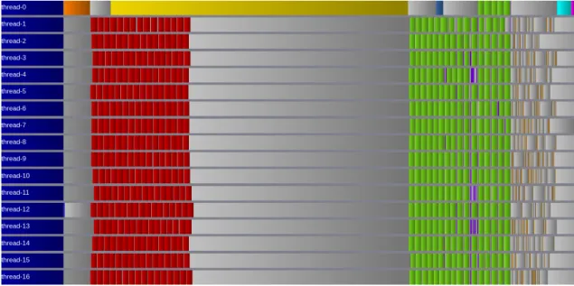
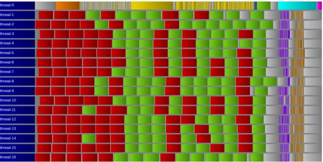
Figure 1: Task scheduling of one iteration of the task variant within only one MPI process (as all processes perform perform the same algorithm in a SPMD fashion) and using on 16 nodes. The orange task is the ghost exchange start-up. Red tasks are the computation of tile interior points. The (very small) dark blue task is the computation of the diagnostics. The yellow task wait for all ghost to be exchanged. green tasks are the computation of tile border points. The blue task wait for all ghosts to be sent. Purple tasks swap tiles and prepare MPI buffer to be sent. Brown tasks are local ghost copies. The cyan task perform the allreduce operations required for performing the poison task in magenta. Grey areas are either idle time or submission time. The master thread is the thread 0.
Figure 1 show the task schedule of one iteration of the task-based variant. We can see that the overall schedule is far from optimal: a significant part of the completion time is wasted either to submit tasks (master thread) or to wait for tasks to be completed (workers threads).
5.1.2 Computation/Communication interleaving
In order to improve improve the overall schedule, a first step consists in moving the submission of interior-point tasks ahead since workers are starving. Then, another step consists in interleaving the MPI Wait calls (when needed) with the submission of the border point tasks so that they can be executed during MPI communications. Thus, we expect the first step move the execution of the interior point tasks ahead so workers can be available to execute the border point tasks which should also be moved ahead thanks to a better overlapping.
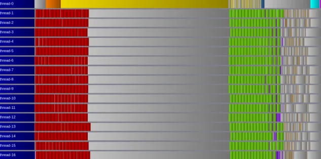
Figure 2 shows that our expectation are unfortunately not fulfilled. Indeed, while workers can execute interior point earlier, the border point tasks are still executed lately because of a too slow initial MPI Wait in each iteration. The overall execution time for this task new version is 25.48 s. Moreover, we can see on Figure 2 that tasks relative to the ghost copy are very fine-grained and that they submission take a significant time (mainly caused by the additional cost of dependencies). Consequently, the master does not submit tasks quickly enough and workers are starving, slowing down the whole execution.
5.1.3 Reducing the critical path
To reduce the submission time in the master thread, we choose to move the ghost-copy task submission away from on the critical path at the expense of additional over-synchronizations. Indeed, by adding a synchronization before tasks that prepare sending buffers and before tasks
Figure 2: Task scheduling of one iteration of the task variant within only one MPI process using on 16 nodes. The legend is same than Figure 1.
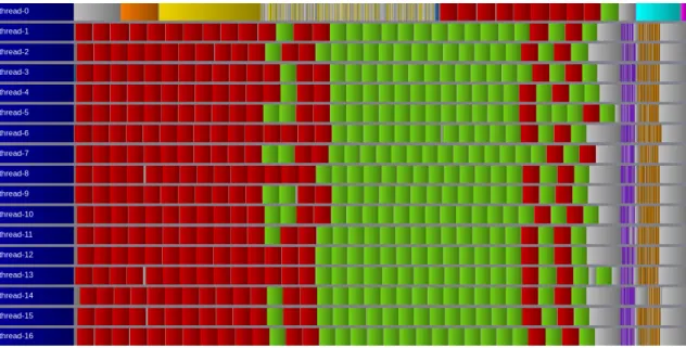
Figure 3: Task scheduling of one iteration of the task variant within only one MPI process using on 16 nodes. The legend is same than Figure 1.
that copy buffers, all dependencies of such tasks can be removed which results in a significantly faster submission time. Moreover, these tasks can be submitted in another thread (thanks to the new synchronizations) so that the master thread can perform the allreduce operations while workers copy local ghosts. All of this is simply done by submitting tasks containing a task loop directive.
It is important to note that OpenMP allows the runtime to merge tasks of the task loop (under certain conditions) to reduce the overhead even though few runtimes actually able to do it. The runtime we choose is not yet able to perform this optimization.
Figure 3 shows that this optimization significantly reduces the submission time on the critical path, thus improving the overall completion time of the task version to 22.45 s.
5.1.4 Data distribution
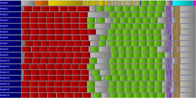
Figure 4: Task scheduling of one iteration of the task variant within only one MPI process using on 16 nodes. The legend is same than Figure 1.
The biggest problem that can be observed on Figures 2 and 3 is the slow initial MPI Wait in each iteration. To fully understand why the ghost exchange is slow and how it can be improved we need to carefully consider the communication patterns and the data distribution.
The communication pattern for the advection is a halo exchange where the 8 neighbors of each cell exchange their ghost area. The whole set of tile is split along the dimension v when the number of process is smaller than the number of tile along this dimension. Conversely, when the number of process is bigger, the set of tile is first split along the dimension v to form tile lines then split again along the dimension x.
For a given tile size, the amount of data transfered as well as the number of message exchanged is proportional to the number of tiles on the edge of the local dataset in each process. Thus, the bigger the perimeter of the local dataset, the slower the communication time. This means that the current data decomposition is not well suited. A 2D decomposition with a balanced number of tiles along each dimension could be more efficient. The theoretical speedup of this new decomposition over the old one is O(
√ p
2 ) for the amount of data transfered and O(
√
p) for the number of messages exchanged, where p is the number of processes.
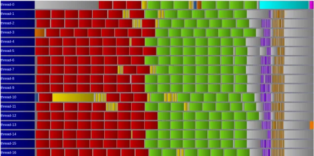
Figure 4 displays the results obtained with the new 2D data distribution. We can see that this version is able to fully overlap the ghost exchange with computations thanks to faster communi-cations. This optimization can be applied on both variants and drastically speed up their overall completion time to 10.73 s for the loop-based variant and 10.87 s for the task-based variant.
Figure 5 shows the same version executed on 32 nodes (still with the same parameters). Due to a higher number of processes, there is almost two times less data to compute per process while the amount of data transfered is just slightly reduced. As a result, communications begin to bound again the overall execution since achieving a good overlapping in such a condition is more challenging. The overall completion time on both variants is now respectivelly 6.37 s and 6.45 s.
5.1.5 Task & Message reordering
We can see on Figure 5 that most of workers are starving after having executed all of the interior point tasks. Indeed, the master thread is stuck on waiting for ghosts to be received (especially the
Figure 5: Task scheduling of one iteration of the task variant within only one MPI process using on 32 nodes. The legend is same than Figure 1.
Figure 6: Task scheduling of one iteration of the task variant within only one MPI process using on 32 nodes. The legend is same than Figure 1.
first) and does not feed workers quickly enough while after that it submit almost all the remaining border point tasks at once.
Balancing the submission throughput over time can help overcome this problem. We achieved this by reordering border points tasks using with a cost function associated to each tile. The idea is to submit tasks that does not require MPI communications first. Tiles computed by such tasks have a cost of −1. Then, tasks that require ghosts are submitted regarding the ghost sending order. The cost of each tile t ∈ T is set to maxsendId(t0)|∀t0∈ T, isN eighbor(t0, t) where sendId
is the index of the tile in the ghost sending list (wherein ghost are grouped by tiles). As a result, firstly awaited tasks are those who either do not require MPI communications or are dependent of ghost tile sent early. It is important to note that the ghost sending order has not been changed
in this new version.
Such an optimization also enable MPI implementations that support asynchronous operations to overlap communication with the task submission. Conversely, without the asynchronous sup-port, the communication may start only during the first MPI Wait delaying the ghost exchange that might turn out to slow down the application. Unfortunately, most of MPI implementations does not fully support them in practice. This include unfortunately IntelMPI 2017 actually used in this paper.
Figure 6 display the task scheduling of this new version. Border tasks are executed earlier by workers compared than the previous version and there is almost no idle time during the ghost exchange. Moreover, the time required to await for the ghosts of the first tile has been significantly reduced even though it is still expensive compared to other subsequent tiles. As a result, the overall completion time of this task version is now of 6.31 s, thus slightly faster than the loop-based version.
5.1.6 Reducing the critical path again
Figure 7: Task scheduling of one iteration of the task variant within only one MPI process using on 32 nodes. The legend is same than Figure 1.
The parallel execution of tasks that both fill ghosts and swap buffers delays the allreduce operations on the critical path slowing down the application while they are only required by Poisson (only the buffer swap). It turns out that those tasks can be submitted in another thread using the same method described in Section 5.1.3. The result is exposed in Figure 7. The completion time of this new version is 6.10 s.
It is important to note that we also tried to merge the two allreduce operations into a bigger one and expected to see a slight performance improvement but it was not the case. Thus, previous results do not include this optimization. While this effect has been reproduced on all platforms used in this paper, it is expected to not be the case for all MPI implementations or platforms.
5.1.7 Leveraging MPI THREAD SERIALIZED and task priorities
The last version is mainly limited by the master thread at scale. Indeed, with 32 nodes on Frioul, most its time is spend in MPI communication and the rest of the time is spent to feed workers with tasks. At scale, the pressure on the master thread can result in a load imbalance and thus impair the performances.
Figure 8: Task scheduling of one iteration of the task variant within only one MPI process using on 32 nodes. The legend is same than Figure 1.
Approach A solution to this problem can be to move MPI calls from the master thread by wrapping calls into tasks with dependencies. Although some MPI calls can even be executed concurrently (require the MPI thread level to be MPI THREAD THREAD), many MPI implementations use locks to protect their internal structures. This causes MPI concurrent calls to be partially or fully serialized and thus workers to wait inefficiently while they could execute other tasks in the meantime. As a result, we choose to serialize all MPI tasks using dependencies. On one hand, the asynchronous MPI calls of the ghost exchange is split in two parts: the ghost sending and the ghost reception. Each part is wrapped in a task. The ghost-sending task is submitted just after the allreduce operations while the ghost-reception task is submitted after waiting for all ghost. On the other hand, waiting operations are also wrapped in tasks so that the dependent border tasks can be submitted simultaneously and executed when data are received.
Note on task priorities MPI calls should absolutely be executed as soon as possible for the critical path to be as short as possible. While submitting MPI tasks ahead help to do that, the OpenMP runtime is free to execute them lately. Thus, priorities on MPI tasks as been added to give hints the runtime. Moreover, priorities as also been used to schedule interior task ahead so that dependent border tasks can be executed sooner.
Results Figure 8 show the task scheduling of this new version. We can see that the benefits of this approach is to achieve both the MPI communication and the task submission in parallel in multiple threads (two simultaneously). However, wrapping MPI calls to tasks can introduce latencies between MPI operations (especially between the many waiting calls) that can slightly increase the execution time when MPI calls are on the critical path. The overall execution time of this new task version is 6.03 s.
6
Final Evaluation
6.1
Methods & Experimental Setup
Methods The median completion time of each version of the two variants is retrieved from a set of 10 runs. Each run perform 1000 iterations and works with a tile size of 64x64 over a 2D dataset of 8192x8192.
Name CPUs Network
KNL Xeon Phi KNL 7250 with 68 cores @ 1.40GHz Intel Omni-Path
100 Gb/s (Fat-tree) SKL 2 socket Xeon 8160 (SkyLake) with 24 cores @ 2.1GHz
Table 1: Informations about the two modules of the Marconi supercomputer used.
Configuration The experiments have been performed on multiple modules of the Marconi su-percomputer. Table 1 bring details about the configuration of the hardware. The binding consist in one process per NUMA node (to prevent NUMA effects which are not the scope of this paper) and one thread per core is used unless explicitly stated (no hyper-threading). The software used is the same than in Section 5.1. As in Section 5.1, the tile size is 64x64 and the dataset size is 8192x8192.
6.2
Experimental Results
20 21 22 23 24 25 26 27nodes
101 102time (s)
Variants
blocking-forloop-last forloop-init forloop-last task-init task-last(a) On the KNL architecture
20 21 22 23 24 25 26
nodes
101 102time (s)
Variants
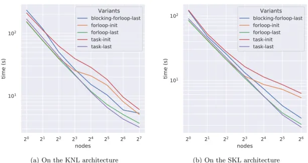
blocking-forloop-last forloop-init forloop-last task-init task-last (b) On the SKL architectureFigure 9: Completion time of each variant over the number of nodes used (strong scaling).
Figure 9a and 9b display the completion time plotted against the number of cores for five variants, respectively on KNL and SKL. There is five variants, split in two groups. On one side, tree loop-based implementations: a naive implementation called “blocking-forloop” that do not overlap communication with computation, a more advanced loop-based implementation called “forloop-init” that perform an overlap communication with computation as much as possible by removing barrier when it is possible which does not take into account all the improvements proposed in this paper (thus, it uses the initial non-2D decomposition) and the “forloop-last” based on the previous one that includes the improvements (only the 2D decomposition for this implementation). On the other side, two task-based implementations following the same principle: an initial “task-init” implementation without the proposed improvements and the more advanced “task-last”
implementation that include them. The two task-based versions also overlap communication with computation.
First of all, these two figures show that the last implementations scales well up to 128 and 64 nodes (respectively 8704 and 3072 cores) regarding to the small size of the dataset, while the naive and initial implementations does not as much (respectively due to the poor overlapping and the inefficient initial decomposition). For all variants, the main cause of the scalability issues lies in the slow sequential resolution of Poisson: the allreduce operations does not scale well with the number of core and they are overlapped less computation as the number of nodes grows. Indeed, the allreduce operations of the task-based implementation take 47% of the overall execution time with 128 nodes on KNL, with only less than 5% of overlapping during this phase.
Moreover, we can see that the last loop-based variant outperform the last task-based one with a small number of nodes (up to respectively 12% and 8% faster on KNL and SKL). However, the last task-based variant scale better than the others and can even outperform the last loop-based variant when using a high number of nodes (up to respectively 18% and 11% faster on KNL and SKL). It is not surprising as the task-based implementation has been design to achieve a better overlapping and thus to scale better. The slowdown of this variant comes from the submission time of the ghost-exchange related tasks executed during the computation of Poisson: Poisson is faster than the submission with few nodes and slower with many nodes. While the submission can be moved ahead, it comes at a high cost, that can slow all the overall execution down, especially when a large number of thread is used. Nevertheless, the last task-based implementation is respectively 67% and 38% faster on KNL and SKL than the naive loop-based version which demonstrates the benefits of overlapping communication with computation using OpenMP tasks.
6.3
Parameter Tunning
1 2 4 8 16 32 64 128nodes
64x32 64x64 128x64 128x128 256x128 256x256block size (width x height)
1.01.2 1.4 1.6 1.8 2.0
(a) Normalized time (ratio) of the task-based variant plot-ted against both the tile size and the number of nodes. For each set of nodes, the time is normalized to the best tile size (in the list). All ratio are clamped to the maxi-mum value 2. 20 21 22 23 24 25 26 nodes 0.90 0.95 1.00 1.05 1.10 1.15 1.20 1.25 hyper-threading speedup Variants forloop-last task-last
(b) Speedup of using two threads/core
Impact of the tile size Figure 10a displays the overhead coming from the choice of the tile size regarding the number of nodes used to run the task-based variant. Such an overhead include the management of ghosts, runtime costs (e.g. task scheduling), hardware effects (e.g. cache effects). We can see that the most efficient tile size clearly depends of the number of nodes. We can also emphasizes that the cost of an under-decomposition of the domain is clearly more prohibitive than an over-decomposition. Thus, it is better to perform a slight over-decomposition that give more freedom to the runtime than being the subject of significant overheads. It is worth noting that the tile size of 64x64 chosen in Sections 5 and 6.2 is not always optimal but is a good candidate for analyzing scalability of this application up to 128 nodes.
Impact of the hyper-threading Figure 10b shows the speedup of using two threads per core rather than one on KNL for the last version of the both variants (with still the same tile size). Overall, enabling hyper-threading helps to significantly reduce the completion time of both variant on few nodes (up to 23% for the loop-based implementation and 27% for the task-based one). However, the benefits are fading as the number of nodes increases. Indeed, hyper-threading does not speed-up communications, which become predominant as the application scale. Even worse, it slows communications down as the threads that perform communications share a core with another. As a result, communications bound the completion time with fewer nodes than without hyper-threading. As the task-based variant is able to better overlap communication with computation, this implementation results in higher performance boost with hyper-threading compared to the loop-based one. Still, a particular attention should be paid to the submission time as is may be so big that workers can starve and increase overheads, especially since the submission is slowed down by hyper-threading as well as the potential extra tiles needed to feed the additional threads. Moreover, more tiles are needed to feed the additional threads, impacting the optimal tile size (a smaller tile size may not always be better due to the higher overheads and the limited benefits of enabling hyper-threading). Finally, hyper-threading provide no benefits with an optimal-chosen tile size on 64 and 128 nodes for both variants.
6.4
Discussion
OpenMP features and limitations Using task priorities in the task-based variant significantly helps to cut the critical path down by moving communication tasks away of it. However, some implementations do not currently support task priorities (the default LLVM/Intel runtime does not, but KOMP and GNU OpenMP implementation support them). When no support is provided, the previous version (without priorities) should be used. Some additional features brought by the OpenMP 5.0 standard can help to design a better and cleaner implementation (and might also improve performance with some runtime). First of all, it provide a direct way to wait a specific task which is more readable and efficient than the current method based on the creation of an undeferred task with dependencies. Moreover, this new OpenMP version also bring a way to bind tasks to places (such as cores) so that all MPI tasks can run on a specific set of threads rather than moving between them. This can improve performance by preserving locality and reducing latency if some thread are dedicated to MPI communication. When hyper-threading is enabled, such a method can even speed communications up if two dedicated cores are reserved for both the task submission and communication tasks. Finally, the task submission is a matter of concerns: the current OpenMP version prevent the submission of a connected graph of tasks (where nodes are tasks and arcs are dependencies) in multiple threads as task dependencies. Consequently, the submission is bound to be sequential in our case. Moreover, since there should be enough task per threads to feed them, the size of the submitted graph for each iteration can be quite big. The problem is that the sequential submission of this big graph can take a significant time for each iteration (as there is no way with OpenMP to specify that all iterations produce the same graph) and thus can result in a worker starvation. This problem will probably be worse in a near future as the number of core per node is expected to be higher in order to reach exascale supercomputers.
Synchronization overheads The methods ensuring thread synchronizations in both variants introduces substantial overheads. One one side, the loop-based approach intensively uses barriers to achieve synchronizations. However, barriers cause scalability issues on many-cores architectures since the slowest thread to slow down all other and the thread computation time often is perturbed by many factors (load balancing, system, frequency scaling, hardware events...). On the other side, the task-based approach mainly uses dependencies to perform local synchronizations. While local synchronization should bring a better scalability, task dependencies does not come for free: they significantly slow down the submission time. A huge submission time can cause worker threads to starve, increasing the overall execution time. Submitting more task (e.g. finer-grained computation) and using more worker threads (e.g. with hyper-threading) make the situation worse. As a result, the amount of dependency per task should be minimized. Sometimes, it should be
done at the expense of the code maintainability (e.g. indirect dependencies, over-synchronization, control-based dependencies).
Code readability and maintainability First of all, while the blocking version of the loop-based variant is the simplest and the easiest to maintain, it is also one of the most inefficient. Moreover, removing most of explicit barriers and implicit barriers of OpenMP parallel loops, that results in the loop-based variant with overlapping, is not easy and very bug prone. Indeed, with most barriers removed, several portions of the code can be executed in different threads and all possible states of the threads should be tracked to prevent race conditions. The problem is that most synchronizations are either implicit or are over-synchronizations. Task dependencies in the task-based variant help to explicitly define local synchronizations and are more flexible than barriers. But the task-based variant is also a bit more complex.
Additional remarks The current application use a regular mesh. In such a situation, the loop-based variant is good condition and thus it is challenging for the task-loop-based to perform better. However, we expect the task-based variant to be more useful with irregular meshes since the workload is not uniformly distributed amongst the tasks. This project is part of a bigger one and is one step toward designing a newer version of Gysela intended to use an irregular mesh.
7
Conclusion
This paper has studied the use of OpenMP task constructs to achieve an efficient and maintainable overlapping of MPI communication with computation and compare it to the use of work-sharing constructs. The benefits and overheads of the variants have been exhibited throughout the specific setting of a hybrid MPI+OpenMP 2D Vlasov-Poisson application.
Experiments demonstrate that using OpenMP tasks help to reach a better overlapping of communication with computation compared to the use of loop-based OpenMP constructs. Results show a completion-time improvement when many nodes are used: from 11%, up to 27%. Those results are tempered with the increased complexity of the code introduced by the additional asynchronism.
We have discussed the capabilities and the limitations of OpenMP 4.5. We expect the fu-ture versions to mitigate the submission problem. While we have mentioned some benefits of using OpenMP 5.0, a deeper exploration is needed. It can also be interesting to study whether alternative communication methods such as shared-memory halo-based communications can give similar results with respect to a task-based overlapping. More complex use-cases can be analyzed, especially the ones with more complex solvers and using irregular meshes.
References
[1] Fran¸cois Broquedis, Thierry Gautier, and Vincent Danjean. Libkomp, an efficient openmp runtime system for both fork-join and data flow paradigms. In Proceedings of the 8th Inter-national Conference on OpenMP in a Heterogeneous World, IWOMP 2016, pages 102–115, Berlin, Heidelberg, 2012. Springer-Verlag.
[2] Nicolas Crouseilles, Guillaume Latu, and Eric Sonnendr¨ucker. Hermite spline interpolation on patches for parallelly solving the Vlasov-Poisson equation. International Journal of Applied Mathematics and Computer Science, 17(3):335–349, 2007.
[3] F. Filbet and E. Sonnendr¨ucker. Comparison of Eulerian Vlasov solvers. Computer Physics Communications, 150(3):247 – 266, 2003.
[4] OpenMP Architecture Review Board. OpenMP Application Programming Interface Version 4.5, November 2015.
[5] Eric Sonnendr¨ucker, Jean Roche, Pierre Bertrand, and Alain Ghizzo. The semi-Lagrangian method for the numerical resolution of the Vlasov equation. Journal of Computational Physics, 149(2):201 – 220, 1999.