HAL Id: hal-01957617
https://hal.laas.fr/hal-01957617
Submitted on 17 Dec 2018
HAL is a multi-disciplinary open access
archive for the deposit and dissemination of
sci-entific research documents, whether they are
pub-lished or not. The documents may come from
teaching and research institutions in France or
abroad, or from public or private research centers.
L’archive ouverte pluridisciplinaire HAL, est
destinée au dépôt et à la diffusion de documents
scientifiques de niveau recherche, publiés ou non,
émanant des établissements d’enseignement et de
recherche français ou étrangers, des laboratoires
publics ou privés.
Leaves Segmentation in 3D Point Cloud
William Gélard, Ariane Herbulot, Michel Devy, Philippe Debaeke, Ryan
Mccormick, Sandra Truong, John Mullet
To cite this version:
William Gélard, Ariane Herbulot, Michel Devy, Philippe Debaeke, Ryan Mccormick, et al.. Leaves
Segmentation in 3D Point Cloud. Advanced Concepts for Intelligent Vision Systems 18th International
Conference, ACIVS 2017, Antwerp, Belgium, September 18-21, 2017, Proceedings, pp.664-674, 2017.
�hal-01957617�
Leaves segmentation in 3D point cloud
William G´elard1,2,3, Ariane Herbulot1,2, Michel Devy1, Philippe Debaeke3,
Ryan F. McCormick4, Sandra K. Truong4, and John Mullet4 1
CNRS, LAAS, 7 avenue du colonel Roche, F-31400 Toulouse, France
2
Univ de Toulouse, UPS, LAAS, F-31400 Toulouse, France
3 INRA, AGIR, 24 Chemin de Borde Rouge, F-31326 Castanet-Tolosan, France 4
Interdisciplinary Program in Genetics and Biochemistry and Biophysics Department, Texas A&M University, College Station, Texas 77843 Email: {wgelard,herbulot,devy}@laas.fr, [email protected],
{ryanabashbash,thkhavi,jmullet}@tamu.edu
Abstract. This paper presents a 3D plant segmentation method with an emphasis on segmentation of the leaves. This method is part of a 3D plant phenotyping project with a main objective that deals with the development of the leaf area over time. First, a 3D point cloud of a plant is obtained with Structure from Motion technique and the cloud is then segmented into the main components of a plant: the stem and the leaves. As the main objective is to measure leaf area over time, an emphasis was placed on accurate segmentation and the labelling of the leaves. This article presents an original approach which starts by finding the stem in a 3D point cloud and then the leaves. Moreover, this method relies on the model of a plant as well as the agronomic rules to affect a unique label that do not change over time. This method is evaluated using two morphologically distinct plants, sunflower and sorghum.
1
Introduction
During the last decade, the efforts made to meet the increasing food demand have led to the development of genotyping methods allowing the biologists to obtain a better understanding of the genetic basis of crop traits. Looking for adaptation to climate change and more sustainable agriculture have oriented research to a better understanding of the relationships between genotype (DNA) and phenotype (visual characteristics) in a given environment in order to speed up and focus plant breeding [1, 3]. Currently, the main phenotyping methods are manual, invasive and sometimes destructive. In an effort to improve the association between genotype and phenotype data, recent studies move toward the development of automatic phenotyping methods.
With the aim to study the drought resistance of sunflowers, the French Na-tional Institute for Agricultural Research (INRA) has developed a semi-isolated platform allowing the scientists (agronomists and biologists) to monitor up to 1300 pots. In order to automatize the extraction of visual characteristics of plants, recent studies trended towards the use of 3D data [10, 18, 9] and some others like [9, 18] proved that the use of Structure from Motion was well adapted
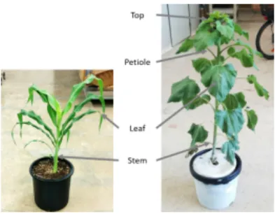
Fig. 1. Description of plants
in 3D plant reconstruction. With this in mind, we previously presented a model-based segmentation of 3D point cloud for phenotyping sunflower plants [7]. In this paper, we present the background in 3D plant acquisition and segmentation and put the emphasis on the development of a model-based segmentation method to segment and label the leaves of a sunflower from 3D data. This method relies on the extraction of the stem from a dense point cloud obtained with Struc-ture from Motion technique and multi-view stereo software. Once the stem was removed from the point cloud, the leaves were segmented by applying an Eu-clidean segmentation which gave good results, but still has some limitations, especially to segment the leaves that are in contact and the leaves at the top of the sunflower plant.
Here, we present a new stem segmentation method and a technique to be able to better segment the leaves that are in contact. Moreover, an effort have been made to bring genericity to the method to be able to work on dicots and monocots plants and this paper shows the results obtained on sunflower (a dicot) and sorghum (a monocot).
This paper is organized as follows: section 2 presents the current method, i.e. stem segmentation and leaves clustering as well as a brief reminder of the previ-ous stem segmentation algorithm, this section also shows the results obtained on sunflower and sorghum. Section 3 draws conclusions on the use of this method and provide guidelines for further works.
2
Method & Results
The method presented in this article deals with the segmentation of plants into several parts, here, sunflowers and sorghum (see Figure 1):
– Main stem, the primary plant axis.
– Leaf: an unstructured thin and more or less elongated object.
– Petiole: a thin stalk from the main stem to a leaf (for sunflower only). – Top: part at the stem extremity, where young leaves appear around the
Fig. 2. Description of the crown in stem segmentation
The starting point of this method is a 3D dense point cloud obtained with OpenMVG [12] and PMVS/CMVS [5, 6], Structure from Motion and Multi-view stereo software. Moreover, in order to retrieve automatically the scale and orientation of the point cloud, we have modified the tool provided by OpenMVG called Ground Control Points registration, a tool that allows a user to manually correct the scale and orientation thanks to a specific pattern or object placed into the scene. To automate this process, we placed a chessboard into the scene and used OpenCV [8] (an image processing library) to locate it. In this way, we are able to automatically retrieve the scale and the orientation of the scene, now the reference frame is given by the chessboard and is centered at the foot of the stem with the x/y-axis aligned on the ground and z-axis aligned along the stem. With an aim to compute the leaf area, the proposed method is only focused on the leaves segmentation. This method relies on the topology of a plant, i.e., a plant is composed of a stem and leaves as made in [15, 19, 14, 7].
First, we will briefly revisit the stem segmentation approach used in [7] and its limitations, then we will present the updated stem segmentation that better fits the shape of a stem. After that, we will revisit how we previously segmented and labelled the leaves in [7] and how we have improved the leaves segmentation.
2.1 Stem segmentation
The idea presented in [7] was to find and remove the stem in a 3D point cloud in order to ease the segmentation of the leaves. To do that, we used a ring with a fixed radius (defined in advance: relying on the botanical model of a plant). This ring is then extended into a cylindrical crown in order to be able to detect the start of the petiole (the insertion part/beginning of the petiole on the stem). This insertion part of the petiole on the stem is then used to label the leaves (see section 2.2 for more details on the labelling step). This crown starts from the foot of the stem and climbs along the stem to reach the top by using a geometrical contraints: the points inside the ring (according to the 2D distance along the z-axis) are assigned as stem (the points inside the radius stem) and the points inside the crown (the points included between the radius stem & radius petiole) are assigned as petiole (see Figure 2).
In general this algorithm gave good results, but it also had some limitations. For example, at the top of the sunflower, where the young leaves appear, the diameter of the stem decreases but the algorithm does not take into account
this parameter and as a result, the beginning of the small leaves are classified as petiole. Another limitation came from the alignment of the direction of the crown with the z-axis, it is a strong constraint that relies on the hypothesis that a stem is straight, and even if it does not affect the result of the leaves segmentation as explained in [7], it is always better to have an algorithm that fits the true shape of a stem.
In order to have an algorithm that better fits the shape of a stem, we improved our stem segmentation algorithm in order to take into account the variability of the diameter of a stem as well as its curvature.
This version of the algorithm relies on the same idea as the previous version, i.e. a cylindrical crown that climbs along a stem, but this time, the radius of the crown is not fixed, it is estimated at each step by using a RANSAC (RANdom SAmple Consensus) [4], an estimating method to find the parameters of a math-ematical model, in this case, a sphere. Moreover, at each step, a center of the crown was computed as well as a direction vector in order to take into account the curvate of a stem. See the algorithm 1 for more details.
Algorithm 1: Stem segmentation Version 2: Adaptative stem segmenta-tion
input : A point cloud output : stem, petioles parameters: height crown
1 // Locate the start of the stem
2 stemBeginning ← initStem ();
3 // Get crown parameters: Centroid + Direction
4 crownParameters ← affineInitStem (stemBeginning);
5 // Start looking for the stem 6 do
7 // Get petiole and stem points
8 crown ← stemClimbing (crownParameters);
9 // Locate a sphere in crownCloud: Center + Radius
10 sphereParameters ← locateSphere (crown);
11 // Check if neighbours are available
12 validNeighbours ← getValidNeighbours (crowParameters, sphereParameters, height crown);
13 // Locate a sphere in the neighborhood
14 sphereParameters ← locateSphere (validNeighbours);
15 // Get the next parameters for the crown
16 crownParameters ← afineCrownParameters (crowParameters, sphereParameters);
17 while haveReachedTop () 6= true;
This improvement takes the stem curvature into account and does not over-flow the petiole, resulting in a well segmented stem as observed in Figure 3.
(a) Sunflower (b) Sorghum
Fig. 3. Example of the adaptative stem segmentation
2.2 Leaves segmentation & Labelling
In this section, we briefly revisit how we segmented and labelled the leaves in [7].
Once we perform the stem segmentation algorithm we have: – The original point cloud.
– The indices of the points assigned as stem (in blue on the figures). – The indices of the points assigned as petioles (in red on the figures).
Euclidean segmentation: At this point, we can remove the points affected as stem in the original point cloud in order to have a point cloud of the plant without the stem. Indeed, because we remove the stem in the original point cloud, we have added/created distances and the leaves can be easily segmented by applying an Euclidean Cluster Extraction [17], a segmentation method based on geometric constraint. And the results can be seen in Figure 4(a). The problem is that the leaves that are in contact are merged in a same cluster (see Figure 4(b) and 4(c)).
To solve this problem, we first need to be able to detect it. To do that, we will use the information from the labelling step.
Leaves labelling: In order to label the leaves, we used the architectural model of a sunflower plant as explain in [7, 16] which states: A unique id can be as-signed according to the insertion height of the leaves on the stem and of the phyllotaxic angles between two successive leaves (the relative angle between two leaves around the stem: see Figure 5(a)).
To achieve this, we used the insertion points of the petioles (labeled red in the figures) obtained at the stem segmentation step and applied an Euclidean segmentation on them. As a result we have merged in different clusters the points that represent the onset of each petiole as possible to see in Figure 5(b). With
(a) Leaf clustering (b) Leaves merged in a same cluster (Sunflower)
(c) Leaves merged in a same cluster (Sorghum)
Fig. 4. Example of results of the leaves segmentation algorithm
(a) phyllotaxic angle (b) petiole clustering
Fig. 5. Illustration of petiole clustering
those clusters, it is possible to obtain the insertion height of each petioles and to compute their phyllotaxic angle which will be then used at the labelling step. Once the onset of the petiole had been labelled, these labels were propagated to the leaves, each leaf cluster receiving the label of the nearest petiole. I some cases, we detected that several petiole clusters were attributed to the same leaf cluster, which needs some more refinement.
Fine leaves segmentation With the aim to solve the problem of leaves merged in a same cluster, we developed a method that relies on the idea brought up in [11] which consists in segmenting the leaves by using a region growing approach. The starting point of the algorithm is a 3D mesh of a plant which is decomposed into
super-voxel [13] and used the connectivity between them to segment the leaves. For that purpose, the stem needs to be already labelled. With this approach it was difficult to make out the leaves from the stem, and because of the topology of the plant (in their case a sorghum), it was easier to manually label the stem and then run the algorithm. Their idea was to look for the furthest point from the stem base (in term of geodesic distance) and assign it a label, then look for the next furthest point and check if it has a neighbor already labelled or not. If so, it will be receive the same label, if not, a new label will be assigned.
In our case, the stem and the leaves have been already segmented, and with our petiole labelling method, we can detect when several leaves have been merged in a same cluster. We only need to find a way to segment those leaves. In order to achieve this, we started from a 3D point cloud of leaves merged in a same cluster and decomposed it into super-voxel. Those super-voxels were built following three constraints applied to each points as explained in [13]:
– Their normal.
– Their spatial distribution. – Their color.
From those super-voxels, we can get back their adjencies and use them to create a weighted graph composed of:
– The stem base.
– The insertion point of each petiole. – The centroid of each super-voxel.
Then, as made in [11], we used the Dijkstra algorithm [2], to find the shortest path between two vertices in the graph. Firstly, we used this algorithm to find the shortest path between all the centroids of the super-voxels and the stem base, and secondly, to find the shortest path between all centroids and petiole onsets. The idea was to locate the furthest super-voxel centroid of the stem base and assign it the label of its nearest petiole. Moreover a constraint on neighborhood is also used at each step in order to assign a label of the furthest super-voxel centroid depending on:
– Its nearest petiole.
– The label of its neighborhood.
The procedure is described in the algorithm 2 and provide more details about the fine leaves segmentation.
Once the super-voxel was labelled, we propagated the label to all points included in a super voxel. An example of application of this algorithm is shown in Figure 6 and 7.
The limitations of this algorithm came from two main issues: – The resolution of the point cloud.
Algorithm 2: Fine leaves segmentation
input : A 3D point cloud of leaves merged in a same cluster Foot of the stem, beginning of the petioles
output: Segmented leaves
1 // Decomposition of the 3D point cloud into supervoxel
2 superVoxelCloud ← getSuperVoxel (cloud);
3 // Build a graph with the supervoxel centroid, the foot of the stem and the begging of the petiole
4 graph ← buildGraph (superVoxelCloud, stemFoot, petioleBeginning);
5 // Get the shorter path between the super voxel centroid and the foot of the stem
6 listOfSuperVoxelCentroid ← getSuperVoxelCentroid (superVoxelCloud);
7 foreach superVoxelCentroid c in listOfSuperVoxelCentroid do
8 distSuperVoxelCentroidToOrgin[c] ← getShorterPath (graph, stem, c);
9 end
10 labelSuperVoxelCentroid ← ∅; 11 do
12 currentSuperVoxelCentroid ← getFarestSuperVoxelCentroid (listOfSuperVoxelCentroid, distSuperVoxelCentroidToOrgin);
13 foreach petioleOrigine p in listOfPetioleOrigin do
14 distSuperVoxelCentroidToPetiole[p] ← getShorterPath (graph, currentSuperVoxelCentroid, p);
15 end
16 label ← getNearestPetioleLabel (listOfPetioleOrigin, distSuperVoxelCentroidToPetiole);
17 labelNeighborhood ← getLabelNeighborhood (currentSuperVoxelCentroid, labelSuperVoxelCentroid); 18 if labelNeighborhood = ∅ then 19 labelSuperVoxelCentroid[currentSuperVoxelCentroid] ← label; 20 else 21 labelSuperVoxelCentroid[currentSuperVoxelCentroid] ← getBestLabel (label, labelNeighborhood); 22 end
23 remove (currentSuperVoxelCentroid, listOfSuperVoxelCentroid);
(a) Super Voxel Cluster-ing
(b) Super Voxel labelled (c) Leaves segmented
Fig. 6. Example of result of the fine leaves segmentation on sunflower
(a) Super Voxel Clustering
(b) Super Voxel la-belled
(c) Leaves segmented
Fig. 7. Example of result of the fine leaves segmentation on sorghum
In Figure 7(b) we can see that the algorithm missed a part of a leaf but the main reason came from the resolution of the point cloud, we can observe a hole in the cloud and the algorithm is not able to find the connectivity between the two separate parts. As a result, the isolated part was ignored. Another limitaion came from the position of the beginning of the petiole. The results given by the stem segmentation algorithm used to extract the stem and the beginning of the petiole can lead to a bad segmentation of the super voxels that are at the border between two leaves. This issue came from the distance of the beginning of the petiole that can be more or less close to the stem base.
3
Conclusion
This paper described a model-based plant segmentation method applies to mono-cot and dimono-cot plants with an effort made on the development of an original stem segmentation in 3D point cloud acquired via Structure from Motion.
We first introduced our previous stem segmentation algorithm, acknowledg-ing its results and limitations.Then, we showed how this algorithm was improved by taking the curvature and variability of the radius of a stem into account. Af-ter that, we made a brief reminder on how we segmented and labelled the leaves and how we detected a problem of leaves merged in a same cluster. To solve this
problem, we presented a method that employs a supervoxel-based approach, building on an idea presented in [11].
With an aim to better evaluate our method, some tests will be performed with plant scientists in order to compare the classical phenotyping method with our method. In the future, we will work on a way to be less dependent from the position of the beginning of the petiole.
4
Acknowledgements
The authors would like to thank Philippe Burger, Nicolas Langlade and Pierre Casadebaig from INRA, Toulouse, for their participation to this work, through a joint project about high throughput phenotyping of sunflowers and the French National Research Agency (ANR) through the project SUNRISE.
References
1. Dhondt, S., Wuyts, N., Inz´e, D.: Cell to whole-plant phenotyping: the best is yet to come. Trends in Plant Science 18(8), 428–439 (2013)
2. Dijkstra, E.W.: A note on two problems in connexion with graphs. Numerische Mathematik 1, 269–271 (1959)
3. Fiorani, F., Schurr, U.: Future Scenarios for Plant Phenotyping. Annual review of plant biology 64, 267–291 (2013)
4. Fischler, M.A., Bolles, R.C.: Random sample consensus: A paradigm for model fitting with applications to image analysis and automated cartography. In: Read-ings in Computer Vision: Issues, Problems, Principles, and Paradigms, p. 726740. Morgan Kaufmann Publishers Inc. (1987)
5. Furukawa, Y., Curless, B., Seitz, S.M., Szeliski, R.: Towards internet-scale multi-view stereo. In: CVPR (2010)
6. Furukawa, Y., Ponce, J.: Accurate, dense, and robust multi-view stereopsis. IEEE Trans. on Pattern Analysis and Machine Intelligence 32(8), 362–1376 (2010) 7. G´elard, W., Devy, M., Herbulot, A., Burger, P.: Model-based segmentation of 3d
point clouds for phenotyping sunflower plants. In: Proceedings of the 12th Inter-national Joint Conference on Computer Vision, Imaging and Computer Graphics Theory and Applications. pp. 459–467 (2017)
8. Itseez: Open source computer vision library (2015), https://github.com/itseez/opencv
9. Jay, S., Rabatel, G., Hadoux, X., Moura, D., Gorretta, N.: In-field crop row pheno-typing from 3d modeling performed using structure from motion. Computers and Electronics in Agriculture 110, 70–77 (2015)
10. Louarn, G., Carr´e, S., Boudon, F., Eprinchard, A., Combes, D.: Characterization of whole plant leaf area properties using laser scanner point clouds. In: Fourth International Symposium on Plant Growth Modeling, Simulation, Visualization and Applications (2012)
11. McCormick, R.F., Truong, S.K., Mullet, J.E.: 3d sorghum reconstructions from depth images identify qtl regulating shoot architecture. Plant Physiol 172(2), 823– 834 (2016)
12. Moulon, P., Monasse, P., Marlet, R., Others: Openmvg. an open multiple view geometry library. (2013), https://github.com/openMVG/openMVG
13. Papon, J., Abramov, A., Schoeler, M., W¨org¨otter, F.: Voxel cloud connectivity segmentation - supervoxels for point clouds. In: Computer Vision and Pattern Recognition (CVPR), 2013 IEEE Conference on (2013)
14. Paproki, A., Sirault, X., Berry, S., Furbank, R., Fripp, J.: A novel mesh processing based technique for 3d plant analysis. BMC Plant Biology 12(1), 63 (2012) 15. Paulus, S., Dupuis, J., Mahlein, A.K., Kuhlmann, H.: Surface feature based
classi-fication of plant organs from 3d laserscanned point clouds for plant phenotyping. BMC Bioinformatics 14(1), 1–12 (2013)
16. Rey, H., Dauzat, J., Chenu, K., Barczi, J.F., Dosio, G.A.A., Lecoeur, J.: Using a 3-d virtual sunflower to simulate light capture at organ, plant and plot levels: Con-tribution of organ interception, impact of heliotropism and analysis of genotypic differences. Ann Bot 101(8), 1139–1151 (2008)
17. Rusu, R.B.: Semantic 3D Object Maps for Everyday Manipulation in Human Liv-ing Environments. Ph.D. thesis, Computer Science department, Technische Uni-versitaet Muenchen, Germany (2009)
18. Santos, T.T., Oliveira, A.A.: Image-based 3d digitizing for plant architecture anal-ysis and phenotyping. In: Workshop on Industry Applications (WGARI) (2012) 19. Wahabzada, M., Paulus, S., Kersting, K., Mahlein, A.K.: Automated interpretation
of 3d laserscanned point clouds for plant organ segmentation. BMC Bioinformatics 16(1), 1–11 (2015)