HAL Id: inria-00360768
https://hal.inria.fr/inria-00360768v3
Submitted on 14 Nov 2009
HAL is a multi-disciplinary open access
archive for the deposit and dissemination of
sci-entific research documents, whether they are
pub-lished or not. The documents may come from
teaching and research institutions in France or
abroad, or from public or private research centers.
L’archive ouverte pluridisciplinaire HAL, est
destinée au dépôt et à la diffusion de documents
scientifiques de niveau recherche, publiés ou non,
émanant des établissements d’enseignement et de
recherche français ou étrangers, des laboratoires
publics ou privés.
A formally verified compiler back-end
Xavier Leroy
To cite this version:
Xavier Leroy. A formally verified compiler back-end. Journal of Automated Reasoning, Springer
Verlag, 2009, 43 (4), pp.363-446. �10.1007/s10817-009-9155-4�. �inria-00360768v3�
(will be inserted by the editor)
A formally verified compiler back-end
Xavier Leroy
Received: 21 July 2009 / Accepted: 22 October 2009
Abstract This article describes the development and formal verification (proof of semantic preservation) of a compiler back-end from Cminor (a simple imperative inter-mediate language) to PowerPC assembly code, using the Coq proof assistant both for programming the compiler and for proving its soundness. Such a verified compiler is useful in the context of formal methods applied to the certification of critical software: the verification of the compiler guarantees that the safety properties proved on the source code hold for the executable compiled code as well.
Keywords Compiler verification · semantic preservation · program proof · formal methods · compiler transformations and optimizations · the Coq theorem prover
1 Introduction
Can you trust your compiler? Compilers are generally assumed to be semantically trans-parent: the compiled code should behave as prescribed by the semantics of the source program. Yet, compilers—and especially optimizing compilers—are complex programs that perform complicated symbolic transformations. Despite intensive testing, bugs in compilers do occur, causing the compiler to crash at compile time or—much worse—to silently generate an incorrect executable for a correct source program [67, 65, 31].
For low-assurance software, validated only by testing, the impact of compiler bugs is low: what is tested is the executable code produced by the compiler; rigorous testing should expose compiler-introduced errors along with errors already present in the source program. Note, however, that compiler-introduced bugs are notoriously difficult to track down. Moreover, test plans need to be made more complex if optimizations are to be tested: for example, loop unrolling introduces additional limit conditions that are not apparent in the source loop.
The picture changes dramatically for safety-critical, high-assurance software. Here, validation by testing reaches its limits and needs to be complemented or even replaced by the use of formal methods: model checking, static analysis, program proof, etc..
X. Leroy
INRIA Paris-Rocquencourt, B.P. 105, 78153 Le Chesnay, France E-mail: Xavier.Leroy@inria.fr
Almost universally, formal methods are applied to the source code of a program. Bugs in the compiler that is used to turn this formally verified source code into an executable can potentially invalidate all the guarantees so painfully obtained by the use of formal methods. In a future where formal methods are routinely applied to source programs, the compiler could appear as a weak link in the chain that goes from specifications to executables.
The safety-critical software industry is aware of these issues and uses a variety of techniques to alleviate them: even more testing (of the compiler and of the generated executable); turning compiler optimizations off; and in extreme cases, conducting man-ual code reviews of the generated assembly code. These techniques do not fully address the issue and are costly in terms of development time and program performance.
An obviously better approach is to apply formal methods to the compiler itself in order to gain assurance that it preserves the semantics of the source programs. Many different approaches have been proposed and investigated, including paper and on-machine proofs of semantic preservation, proof-carrying code, credible compilation, translation validation, and type-preserving compilers. (These approaches are compared in section 2.)
For the last four years, we have been working on the development of a realistic,
verified compiler called Compcert. By verified, we mean a compiler that is accompanied
by a machine-checked proof that the generated code behaves exactly as prescribed by the semantics of the source program (semantic preservation property). By realistic, we mean a compiler that could realistically be used in the context of production of critical software. Namely, it compiles a language commonly used for critical embedded software: not Java, not ML, not assembly code, but a large subset of the C language. It produces code for a processor commonly used in embedded systems, as opposed e.g. to a virtual machine: we chose the PowerPC because it is popular in avionics. Finally, the compiler must generate code that is efficient enough and compact enough to fit the requirements of critical embedded systems. This implies a multi-pass compiler that features good register allocation and some basic optimizations.
This paper reports on the completion of a large part of this program: the formal verification of a lightly-optimizing compiler back-end that generates PowerPC assembly code from a simple imperative intermediate language called Cminor. This verification is mechanized using the Coq proof assistant [25, 11]. Another part of this program— the verification of a compiler front-end translating a subset of C called Clight down to Cminor—has also been completed and is described separately [15, 16].
While there exists a considerable body of earlier work on machine-checked correct-ness proofs of parts of compilers (see section 18 for a review), our work is novel in two ways. First, published work tends to focus on a few parts of a compiler, such as optimizations and the underlying static analyses [55, 19] or translation of a high-level language to virtual machine code [49]. In contrast, our work emphasizes end-to-end verification of a complete compilation chain from a structured imperative language down to assembly code through 6 intermediate languages. We found that many of the non-optimizing translations performed, while often considered obvious in compiler literature, are surprisingly tricky to prove correct formally.
Another novelty of this work is that most of the compiler is written directly in the Coq specification language, in a purely functional style. The executable compiler is obtained by automatic extraction of Caml code from this specification. This approach is an attractive alternative to writing the compiler in a conventional programming language, then using a program logic to relate it with its specifications. This approach
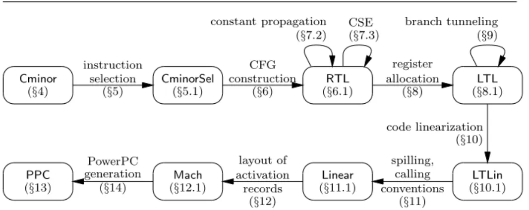
Cminor (§4) CminorSel (§5.1) RTL (§6.1) LTL (§8.1) LTLin (§10.1) Linear (§11.1) Mach (§12.1) PPC (§13) instruction selection (§5) CFG construction (§6) register allocation (§8) code linearization (§10) spilling, calling conventions (§11) layout of activation records (§12) PowerPC generation (§14) constant propagation (§7.2) CSE (§7.3) branch tunneling (§9)
Fig. 1 The passes and intermediate languages of Compcert.
has never been applied before to a program of the size and complexity of an optimizing compiler.
The complete source code of the Coq development, extensively commented, is avail-able on the Web [58]. We take advantage of this availability to omit proofs and a number of low-level details from this article, referring the interested reader to the Coq devel-opment instead. The purpose of this article is to give a high-level presentation of a verified back-end, with just enough details to enable readers to apply similar tech-niques in other contexts. The general perspective we adopt is to revisit classic compiler technology from the viewpoint of the semanticist, in particular by distinguishing clearly between the correctness-relevant and the performance-relevant aspects of compilation algorithms, which are inextricably mixed in compiler literature.
The remainder of this article is organized as follows. Section 2 formalizes various approaches to establishing trust in the results of compilation. Section 3 presents the main aspects of the development that are shared between all passes of the compiler: the value and memory models, labeled transition semantics, proofs by simulation diagrams. Sections 4 and 13 define the semantics of our source language Cminor and our target language PPC, respectively. The bulk of this article (sections 5 to 14) is devoted to the description of the successive passes of the compiler, the intermediate languages they operate on, and their soundness proofs. (Figure 1 summarizes the passes and the intermediate languages.) Experimental data on the Coq development and on the executable compiler extracted from it are presented in sections 15 and 16. Section 17 discusses some of the design choices and possible extensions. Related work is discussed in section 18, followed by concluding remarks in section 19.
2 General framework
2.1 Notions of semantic preservation
Consider a source program S and a compiled program C produced by a compiler. Our aim is to prove that the semantics of S was preserved during compilation. To make this notion of semantic preservation precise, we assume given semantics for the source language Lsand the target language Lt. These semantics associate one or several
divergence, and “going wrong” on executing an undefined computation. (In the remain-der of this work, behaviors also contain traces of input-output operations performed during program execution.) We write S ⇓ B to mean that program S executes with observable behavior B, and likewise for C.
The strongest notion of semantic preservation during compilation is that the source program S and the compiled code C have exactly the same sets of observable behaviors—a standard bisimulation property:
Definition 1 (Bisimulation) ∀B, S ⇓ B ⇐⇒ C ⇓ B.
Definition 1 is too strong to be usable as our notion of semantic preservation. If the source language is not deterministic, compilers are allowed to select one of the possible behaviors of the source program. (For instance, C compilers choose one particular eval-uation order for expressions among the several orders allowed by the C specifications.) In this case, C will have fewer behaviors than S. To account for this degree of freedom, we can consider a backward simulation, or refinement, property:
Definition 2 (Backward simulation) ∀B, C ⇓ B =⇒ S ⇓ B.
Definitions 1 and 2 imply that if S always goes wrong, so does C. Several desirable optimizations violate this requirement. For instance, if S contains an integer division whose result is unused, and this division can cause S to go wrong because its second argument is zero, dead code elimination will result in a compiled program C that does not go wrong on this division. To leave more flexibility to the compiler, we can therefore restrict the backward simulation property to safe source programs. A program S is safe, written Safe(S), if none of its possible behaviors is in the set Wrong of “going wrong” behaviors (S ⇓ B =⇒ B /∈ Wrong).
Definition 3 (Backward simulation for safe programs) If Safe(S), then ∀B, C ⇓ B =⇒ S ⇓ B.
In other words, if S cannot go wrong (a fact that can be established by formal verification or static analysis of S), then neither does C; moreover, all observable behaviors of C are acceptable behaviors of S.
An alternative to backward simulation (definitions 2 and 3) is forward simulation properties, showing that all possible behaviors of the source program are also possible behaviors of the compiled program:
Definition 4 (Forward simulation) ∀B, S ⇓ B =⇒ C ⇓ B.
Definition 5 (Forward simulation for safe programs) ∀B /∈ Wrong, S ⇓ B =⇒ C ⇓ B.
In general, forward simulations are easier to prove than backward simulations (by structural induction on an execution of S), but less informative: even if forward simu-lation holds, the compiled code C could have additional, undesirable behaviors beyond those of S. However, this cannot happen if C is deterministic, that is, if it admits only one observable behavior (C ⇓ B1∧ C ⇓ B2=⇒ B1= B2). This is the case if the target
language Lthas no internal non-determinism (programs change their behaviors only in
response to different inputs but not because of internal choices) and the execution en-vironment is deterministic (inputs given to programs are uniquely determined by their
Bisimulation Backward simulation Safe backward simulation Preservation of specifications Forward simulation Safe forward simulation if C deterministic if S deterministic if C deterministic if S deterministic
Fig. 2 Various semantic preservation properties and their relationships. An arrow from A to
Bmeans that A logically implies B.
previous outputs).1 In this case, it is easy to show that “forward simulation” implies “backward simulation”, and “forward simulation for safe programs” implies “backward simulation for safe programs”. The reverse implications hold if the source program is deterministic. Figure 2 summarizes the logical implications between the various notions of semantic preservation.
From a formal methods perspective, what we are really interested in is whether the compiled code satisfies the functional specifications of the application. Assume that such a specification is given as a predicate Spec(B) of the observable behavior. Further assume that the specification rules out “going wrong” behaviors: Spec(B) =⇒ B /∈ Wrong. We say that C satisfies the specification, and write C |= Spec, if all behaviors of C satisfy Spec (∀B, C ⇓ B =⇒ Spec(B)). The expected soundness property of the compiler is that it preserves the fact that the source code S satisfies the specification, a fact that has been established separately by formal verification of S.
Definition 6 (Preservation of a specification) S |= Spec =⇒ C |= Spec. It is easy to show that “backward simulation for safe programs” implies “preser-vation of a specification” for all specifications Spec. In general, the latter property is weaker than the former property. For instance, if the specification of the application is “print a prime number”, and S prints 7, and C prints 11, the specification is preserved but backward simulation does not hold. Therefore, definition 6 leaves more liberty for compiler optimizations that do not preserve semantics in general, but are correct for specific programs. However, it has the marked disadvantage of depending on the specifications of the application, so that changes in the latter can require the proof of preservation to be redone.
A special case of preservation of a specification, of considerable historical impor-tance, is the preservation of type and memory safety, which we can summarize as “if S does not go wrong, neither does C”:
Definition 7 (Preservation of safety) Safe(S) =⇒ Safe(C).
1 Section 13.3 formalizes this notion of deterministic execution environment by, in effect,
restricting the set of behaviors B to those generated by a transition function that responds to the outputs of the program.
Combined with a separate check that S is well-typed in a sound type system, this property implies that C executes without memory violations. Type-preserving compilation [72, 71, 21] obtains this guarantee by different means: under the assumption that S is well typed, C is proved to be well-typed in a sound type system, ensuring that it cannot go wrong. Having proved a semantic preservation property such as definitions 3 or 6 provides the same guarantee without having to equip the target and intermediate languages with sound type systems and to prove type preservation for the compiler.
In summary, the approach we follow in this work is to prove a “forward simulation for safe programs” property (sections 5 to 14), and combine it with a separate proof of determinism for the target language (section 13.3), the latter proof being particularly easy since the target is a single-threaded assembly language. Combining these two proofs, we obtain that all specifications are preserved, in the sense of definition 6, which is the result that matters for users of the compiler who practice formal verification at the source level.
2.2 Verified compilers, validated compilers, and certifying compilers
We now discuss several approaches to establishing that a compiler preserves semantics of the compiled programs, in the sense of section 2.1. In the following, we write S ≈ C, where S is a source program and C is compiled code, to denote one of the semantic preservation properties 1 to 7 of section 2.1.
2.2.1 Verified compilers
We model the compiler as a total function Comp from source programs to either com-piled code (written Comp(S) = OK(C)) or a compile-time error (written Comp(S) = Error). Compile-time errors correspond to cases where the compiler is unable to pro-duce code, for instance if the source program is incorrect (syntax error, type error, etc.), but also if it exceeds the capacities of the compiler (see section 12 for an example). Definition 8 (Verified compiler) A compiler Comp is said to be verified if it is accompanied with a formal proof of the following property:
∀S, C, Comp(S) = OK(C) =⇒ S ≈ C (i)
In other words, a verified compiler either reports an error or produces code that satisfies the desired semantic preservation property. Notice that a compiler that always fails (Comp(S) = Error for all S) is indeed verified, although useless. Whether the compiler succeeds to compile the source programs of interest is not a soundness is-sue, but a quality of implementation isis-sue, which is addressed by non-formal methods such as testing. The important feature, from a formal methods standpoint, is that the compiler never silently produces incorrect code.
Verifying a compiler in the sense of definition 8 amounts to applying program proof technology to the compiler sources, using one of the properties defined in section 2 as the high-level specification of the compiler.
2.2.2 Translation validation with verified validators
In the translation validation approach [83, 76] the compiler does not need to be veri-fied. Instead, the compiler is complemented by a validator: a boolean-valued function
Validate(S, C) that verifies the property S ≈ C a posteriori. If Comp(S) = OK(C) and Validate(S, C) = true, the compiled code C is deemed trustworthy. Validation can be
performed in several ways, ranging from symbolic interpretation and static analysis of S and C [76, 87, 44, 93, 94] to the generation of verification conditions followed by model checking or automatic theorem proving [83, 95, 4]. The property S ≈ C being undecidable in general, validators must err on the side of caution and should reply falseif they cannot establish S ≈ C.2
Translation validation generates additional confidence in the correctness of the compiled code but by itself does not provide formal guarantees as strong as those provided by a verified compiler: the validator could itself be unsound.
Definition 9 (Verified validator) A validator Validate is said to be verified if it is accompanied with a formal proof of the following property:
∀S, C, Validate(S, C) = true =⇒ S ≈ C (ii)
The combination of a verified validator Validate with an unverified compiler Comp does provide formal guarantees as strong as those provided by a verified compiler. Such a combination calls the validator after each run of the compiler, reporting a compile-time error if validation fails:
Comp′
(S) =
matchComp(S) with
| Error → Error
| OK(C) → if Validate(S, C) then OK(C) else Error
If the source and target languages are identical, as is often the case for optimization passes, we also have the option to return the source code unchanged if validation fails, in effect turning off a potentially incorrect optimization:
Comp′′
(S) =
matchComp(S) with
| Error → OK(S)
| OK(C) → if Validate(S, C) then OK(C) else OK(S)
Theorem 1 If Validate is a verified validator in the sense of definition 9, Comp′
and Comp′′
are verified compilers in the sense of definition 8.
Verification of a translation validator is therefore an attractive alternative to the verification of a compiler, provided the validator is smaller and simpler than the com-piler.
In the presentation above, the validator receives unadorned source and compiled codes as arguments. In practice, the validator can also take advantage of additional information generated by the compiler and transmitted to the validator as part of C or separately. For instance, the validator of [87] exploits debugging information to suggest
2 This conservatism doesn’t necessarily render validators incomplete: a validator can be
a correspondence between program points and between variables of S and C. Credible compilation [86] carries this approach to the extreme: the compiler is supposed to annotate C with a full proof of S ≈ C, so that translation validation reduces to proof checking.
2.2.3 Proof-carrying code and certifying compilers
The proof-carrying code (PCC) approach [75, 2, 33] does not attempt to establish se-mantic preservation between a source program and some compiled code. Instead, PCC focuses on the generation of independently-checkable evidence that the compiled code C satisfies a behavioral specification Spec such as type and memory safety. PCC makes use of a certifying compiler, which is a function CComp that either fails or returns both a compiled code C and a proof π of the property C |= Spec. The proof π, also called a certificate, can be checked independently by the code user; there is no need to trust the code producer, nor to formally verify the compiler itself.
In a naive view of PCC, the certificate π generated by the compiler is a full proof term and the client-side verifier is a general-purpose proof checker. In practice, it is sufficient to generate enough hints so that such a full proof can be reconstructed cheaply on the client side by a specialized checker [78]. If the property of interest is type safety, PCC can reduce to type-checking of compiled code, as in Java bytecode verification [90] or typed assembly language [72]: the certificate π reduces to type annotations, and the client-side verifier is a type checker.
In the original PCC design, the certifying compiler is specialized for a fixed property of programs (e.g. type and memory safety), and this property is simple enough to be established by the compiler itself. For richer properties, it becomes necessary to provide the certifying compiler with a certificate that the source program S satisfies the property. It is also possible to make the compiler generic with respect to a family of program properties. This extension of PCC is called proof-preserving compilation in [89] and certificate translation in [7, 8].
In all cases, it suffices to formally verify the client-side checker to obtain guarantees as strong as those obtained from compiler verification. Symmetrically, a certifying com-piler can be constructed (at least theoretically) from a verified comcom-piler. Assume that
Comp is a verified compiler, using definition 6 as our notion of semantic preservation,
and further assume that the verification was conducted with a proof assistant that pro-duces proof terms, such as Coq. Let Π be a proof term for the semantic preservation theorem of Comp, namely
Π : ∀S, C, Comp(S) = OK(C) =⇒ S |= Spec =⇒ C |= Spec
Via the Curry-Howard isomorphism, Π is a function that takes S, C, a proof of
Comp(S) = OK(C) and a proof of S |= Spec, and returns a proof of C |= Spec. A
certifying compiler of the proof-preserving kind can then be defined as follows:
CComp(S : Source, πs: S |= Spec) =
matchComp(S) with
| Error → Error
| OK(C) → OK(C, Π S C πeq πs)
(Here, πeqis a proof term for the proposition Comp(S) = OK(C), which trivially holds
additional baggage in the definition above that we omitted for simplicity.) The accom-panying client-side checker is the Coq proof checker. While the certificate produced by CComp is huge (it contains a proof of soundness for the compilation of all source programs, not just for S), it could perhaps be specialized for S and C using partial evaluation techniques.
2.3 Composition of compilation passes
Compilers are naturally decomposed into several passes that communicate through intermediate languages. It is fortunate that verified compilers can also be decomposed in this manner.
Let Comp1 and Comp2 be compilers from languages L1 to L2 and L2 to L3,
respectively. Assume that the semantic preservation property ≈ is transitive. (This is true for all properties considered in section 2.1.) Consider the monadic composition of
Comp1 and Comp2:
Comp(S) =
matchComp1(S) with | Error → Error | OK(I) → Comp2(I)
Theorem 2 If the compilers Comp1 and Comp2 are verified, so is their monadic composition Comp.
2.4 Summary
The conclusions of this discussion are simple and define the methodology we have followed to verify the Compcert compiler back-end.
1. Provided the target language of the compiler has deterministic semantics, an ap-propriate specification for the soundness proof of the compiler is the combination of definitions 5 (forward simulation for safe source programs) and 8 (verified com-piler), namely
∀S, C, B /∈ Wrong, Comp(S) = OK(C) ∧ S ⇓ B =⇒ C ⇓ B (i)
2. A verified compiler can be structured as a composition of compilation passes, as is commonly done for conventional compilers. Each pass can be proved sound inde-pendently. However, all intermediate languages must be given appropriate formal semantics.
3. For each pass, we have a choice between proving the code that implements this pass or performing the transformation via untrusted code, then verifying its results using a verified validator. The latter approach can reduce the amount of code that needs to be proved. In our experience, the verified validator approach is particu-larly effective for advanced optimizations, but less so for nonoptimizing translation passes and basic dataflow optimizations. Therefore, we did not use this approach for the compilation passes presented in this article, but elected to prove directly the soundness of these passes.3
3 However, a posteriori validation with a verified validator is used for some auxiliary
heuris-tics such as graph coloring during register allocation (section 8.2) and node enumeration during CFG linearization (section 10.2).
4. Finally, provided the proof of (i) is carried out in a prover such as Coq that gen-erates proof terms and follows the Curry-Howard isomorphism, it is at least theo-retically possible to use the verified compiler in a context of proof-carrying code.
3 Infrastructure
This section describes elements of syntax, semantics and proofs that are used through-out the Compcert development.
3.1 Programs
The syntax of programs in the source, intermediate and target languages share the following common shape.
Programs:
P ::= { vars = id1= data∗1; . . . idn= data∗n; global variables
functs= id1= Fd1; . . . idn= Fdn; functions
main= id } entry point
Function definitions:
Fd ::= internal(F ) | external(Fe) Definitions of internal functions:
F ::= { sig = sig; body = . . . ; . . . } (language-dependent) Declarations of external functions:
Fe ::= { tag = id ; sig = sig } Initialization data for global variables:
data ::= reserve(n) | int8(n) | int16(n)
| int32(n) | float32(f ) | float64(f ) Function signatures:
sig ::= { args = ~τ; res = (τ | void)} Types:
τ ::= int integers and pointers
| float floating-point numbers
A program is composed of a list of global variables with their initialization data, a list of functions, and the name of a distinguished function that constitutes the program entry point (like main in C). Initialization data is a sequence of integer or floating-point constants in various sizes, or reserve(n) to denote n bytes of uninitialized storage.
Two kinds of function definitions Fd are supported. Internal functions F are de-fined within the program. The precise contents of an internal function depends on the language considered, but include at least a signature sig giving the number and types of parameters and results and a body defining the computation (e.g. as a statement in Cminoror a list of instructions in PPC). An external function Fe is not defined within the program, but merely declared with an external name and a signature. External functions are intended to model input/output operations or other kinds of system calls. The observable behavior of the program will be defined in terms of a trace of invocations of external functions (see section 3.4).
The types τ used in function signatures and in other parts of Compcert are ex-tremely coarse: we only distinguish between integers or pointers on the one hand (type int) and floating-point numbers on the other hand (type float). In particular, we make no attempt to track the type of data pointed to by a pointer. These “types” are best thought of as hardware register classes. Their main purpose is to guide register allocation and help determine calling conventions from the signature of the function being called.
Each compilation pass is presented as a total function transf : F1 → (OK(F2) |
Error(msg)) where F1 and F2 are the types of internal functions for the source and
target languages (respectively) of the compilation pass. Such transformation functions are generically extended to function definitions by taking transf(Fe) = OK(Fe), then to whole programs as a monadic “map” operation over function definitions:
transf(P ) = OK {vars = P.vars; functs = (. . . idi= Fd′i; . . .); main = P.main}
if and only if P.functs = (. . . idi= Fdi; . . .) and transf(Fdi) = OK(Fd′i) for all i.
3.2 Values and memory states
The dynamic semantics of the Compcert languages manipulate values that are the discriminated union of 32-bit integers, 64-bit IEEE double precision floats, pointers, and a special undef value denoting in particular the contents of uninitialized memory. Pointers are composed of a block identifier b and a signed byte offset δ within this block.
Values: v ::= int(n) 32-bit machine integer
| float(f ) 64-bit floating-point number | ptr(b, δ) pointer
| undef
Memory blocks: b ∈ Z block identifiers
Block offsets: δ ::= n byte offset within a block (signed)
Values are assigned types in the obvious manner:
int(n) : int float(f ) : float ptr(b, δ) : int undef: τ for all τ The memory model used in our semantics is detailed in [59]. Memory states M are modeled as collections of blocks separated by construction and identified by (math-ematical) integers b. Each block has lower and upper bounds L(M, b) and H(M, b), fixed at allocation time, and associates values to byte offsets δ ∈ [L(M, b), H(M, b)). The basic operations over memory states are:
– alloc(M, l, h) = (b, M′
): allocate a fresh block with bounds [l, h), of size (h − l) bytes; return its identifier b and the updated memory state M′
. – store(M, κ, b, δ, v) = ⌊M′
⌋: store value v in the memory quantity κ of block b at offset δ; return update memory state M′
.
– load(M, κ, b, δ) = ⌊v⌋: read the value v contained in the memory quantity κ of block b at offset δ.
– free(M, b) = M′
: free (invalidate) the block b and return the updated memory M′
. The memory quantities κ involved in load and store operations represent the kind, size and signedness of the datum being accessed:
Memory quantities: κ ::= int8signed | int8unsigned | int16signed | int16unsigned | int32 | float32 | float64
The load and store operations may fail when given an invalid block b or an out-of-bounds offset δ. Therefore, they return option types, with ⌊v⌋ (read: “some v”) denoting success with result v, and ∅ (read: “none”) denoting failure. In this particular instance of the memory model of [59], alloc and free never fail. In particular, this means that we assume an infinite memory. This design decision is discussed further in section 17.4.
The four operations of the memory model satisfy a number of algebraic prop-erties stated and proved in [59]. The following “load-after-store” property gives the general flavor of the memory model. Assume store(M1, κ, b, δ, v) = ⌊M2⌋ and
load(M1, κ′, b′, δ′) = ⌊v′⌋. Then, load(M2, κ ′ , b′, δ′) = 8 < : ⌊cast(v, κ′ )⌋ if b′ = b and δ′ = δ and |κ′ | = |κ|; ⌊v′ ⌋ if b′ 6= b or δ + |κ| ≤ δ′ or δ′ + |κ′ | ≤ δ; ⌊undef⌋ otherwise. The cast(v, κ′
) function performs truncation or sign-extension of value v as prescribed by the quantity κ′
. Note that undef is returned (instead of a machine-dependent value) in cases where the quantities κ and κ′
used for writing and reading disagree, or in cases where the ranges of bytes written [δ, δ+|κ|) and read [δ′, δ′+|κ′
|) partially overlap. This way, the memory model hides the endianness and bit-level representations of integers and floats and makes it impossible to forge pointers from sequences of bytes [59, section 7].
3.3 Global environments
The Compcert languages support function pointers but follow a “Harvard” model where functions and data reside in different memory spaces, and the memory space for func-tions is read-only (no self-modifying code). We use positive block identifiers b to refer to data blocks and negative b to refer to functions via pointers. The operational semantics for the Compcert languages are parameterized by a global environment G that does not change during execution. A global environment G maps function blocks b < 0 to func-tion definifunc-tions. Moreover, it maps global identifiers (of funcfunc-tions or global variables) to blocks b. The basic operations over global environments are:
– funct(G, b) = ⌊Fd ⌋: return the function definition Fd corresponding to the block b < 0, if any.
– symbol(G, id) = ⌊b⌋: return the block b corresponding to the global variable or function name id , if any.
– globalenv(P ) = G: construct the global environment G associated with the pro-gram P .
– initmem(P ) = M : construct the initial memory state M for executing the program P .
The globalenv(P ) and initmem(P ) functions model (at a high level of abstraction) the operation of a linker and a program loader. Unique, positive blocks b are allocated and associated to each global variable (id = data∗
blocks are initialized according to data∗
. Likewise, unique, negative blocks b are asso-ciated to each function definition (id = Fd ) of P . In particular, if the functions of P have unique names, the following equivalence holds:
(id , Fd ) ∈ P.functs ⇐⇒ ∃b < 0. symbol(globalenv(P ), id) = ⌊b⌋ ∧ funct(globalenv(P ), b) = ⌊Fd ⌋
The allocation of blocks for functions and global variables is deterministic so that convenient commutation properties hold between operations on global environments and per-function transformations of programs as defined in section 3.1.
Lemma 1 Assume transf(P ) = OK(P′
). – initmem(P′
) = initmem(P ).
– If symbol(globalenv(P ), id) = ⌊b⌋, then symbol(globalenv(P′
), id ) = ⌊b⌋. – If funct(globalenv(P ), b) = ⌊Fd ⌋, then there exists a function definition Fd′
such that funct(globalenv(P′
), b) = ⌊Fd′
⌋ and transf(Fd ) = OK(Fd′
).
3.4 Traces
We express the observable behaviors of programs in terms of traces of input-output events, each such event corresponding to an invocation of an external function. An event records the external name of the external function, the values of the arguments provided by the program, and the return value provided by the environment (e.g. the operating system).
Events: ν ::= id( ~vν7→ vν)
Event values: vν::= int(n) | float(f )
Traces: t ::= ǫ | ν.t finite traces (inductive)
T ::= ǫ | ν.T finite or infinite traces (coinductive)
Behaviors: B ::= converges(t, n) termination with trace t and exit code n | diverges(T ) divergence with trace T
| goeswrong(t) going wrong with trace t
We consider two types of traces: finite traces t for terminating or “going wrong” executions and finite or infinite traces T for diverging executions. Note that a diverging program can generate an empty or finite trace of input-output events (think infinite empty loop).
Concatenation of a finite trace t and a finite trace t′
or infinite trace T is written t.t′
or t.T . It is associative and admits the empty trace ǫ as neutral element.
The values that are arguments and results of input-output events are required to be integers or floats. Since external functions cannot modify the memory state, passing them pointer values would be useless. Even with this restriction, events and traces can still model character-based input-output. We encapsulate these restrictions in the following inference rule that defines the effect of applying an external function Fe to arguments ~v.
~v and v are integers or floats
~v and v agree in number and types with Fe.sig t = Fe.tag(~v 7→ v)
⊢ Fe(~v)⇒ vt
Note that the result value v and therefore the trace t are not completely determined by this rule. We return to this point in section 13.3.
3.5 Transition semantics
The operational semantics for the source, target and intermediate languages of the Compcert back-end are defined as labeled transition systems. The transition relation for each language is written G ⊢ S → St ′
and denotes one execution step from state S to state S′
in global environment G. The trace t denotes the observable events generated by this execution step. Transitions corresponding to an invocation of an external function record the associated event in t. Other transitions have t = ǫ. In addition to the type of states S and the transition relation G ⊢ S→ St ′
, each language defines two predicates:
– initial(P, S): the state S is an initial state for the program P . Typically, S cor-responds to an invocation of the main function of P in the initial memory state initmem(P ).
– final(S, n): the state S is a final state with exit code n. Typically, this means that the program is returning from the initial invocation of its main function, with return value int(n).
Executions are modeled classically as sequences of transitions from an initial state to a final state. We write G ⊢ S→t+ S′ to denote one or several transitions (transitive
closure), G ⊢ S →t∗
S′
to denote zero, one or several transitions (reflexive transitive closure), and G ⊢ S→ ∞ to denote an infinite sequence of transitions starting with S.T The traces t (finite) and T (finite or infinite) are formed by concatenating the traces of elementary transitions. Formally:
G ⊢ S→ǫ∗S G ⊢ S t1 → S′ G ⊢ S′ t2 →∗ S′′ G ⊢ St1→.t2∗ S′′ G ⊢ S→ St1 ′ G ⊢ S′ t→2∗ S′′ G ⊢ St1→.t2+S′′ G ⊢ S→ St ′ G ⊢ S′ T → ∞ G ⊢ St.T→ ∞
As denoted by the double horizontal bar, the inference rule defining G ⊢ S → ∞ isT to be interpreted coinductively, as a greatest fixpoint. The observable behavior of a program P is defined as follows. Starting from an initial state, if a finite sequence of reductions with trace t leads to a final state with exit code n, the program has observable behavior converges(t, n). If an infinite sequence of reductions with trace T is possible, the observable behavior of the program is diverges(T ). Finally, if the program gets stuck on a non-final state after performing a sequence of reductions with trace t, the behavior is goeswrong(t).
S C R other instructions internal function return instruction
call instruction non-empty call stack
external function Program starts empty call stack Program ends
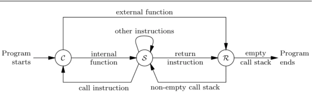
Fig. 3 Transitions between the three kinds of program states.
initial(P, S) globalenv(P ) ⊢ S→t∗ S′ final(S′ , n) P ⇓ converges(t, n) initial(P, S) globalenv(P ) ⊢ S→ ∞T P ⇓ diverges(T ) initial(P, S) globalenv(P ) ⊢ S→t∗ S′ S′ 6→ ∀n, ¬final(S′ , n) P ⇓ goeswrong(t)
The set of “going wrong” behaviors is defined in the obvious manner: Wrong = {goeswrong(t) | t a finite trace}.
3.6 Program states
The contents of a program state vary from language to language. For the assembly language PPC, a state is just a pair of a memory state and a mapping from processor registers to values (section 13.2). For the other languages of the Compcert back-end, states come in three kinds written S, C and R.
– Regular states S correspond to an execution point within an internal function. They carry the function in question and a program point within this function, possibly along with additional language-specific components such as environments giving values to function-local variables.
– Call states C materialize parameter passing from the caller to the callee. They carry the function definition Fd being invoked and either a list of argument values or an environment where the argument values can be found at conventional locations. – Return states R correspond to returning from a function to its caller. They carry
at least the return value or an environment where this value can be found. All three kinds of states also carry the current memory state as well as a call stack: a list of frames describing the functions in the call chain, with the corresponding program points where execution should be resumed on return, possibly along with function-local environments.
If we project the transition relation on the three-element set {S, C, R}, abstracting away the components carried by the states, we obtain the finite automaton depicted in figure 3. This automaton is shared by all languages of the Compcert back-end except PPC, and it illustrates the interplay between the three kinds of states. Initial states
are call states with empty call stacks. A call state where the called function is external transitions directly to a return state after generating the appropriate event in the trace. A call state where the called function is internal transitions to a regular state corresponding to the function entry point, possibly after binding the argument values to the parameter variables. Non-call, non-return instructions go from regular states to regular states. A non-tail call instruction resolves the called function, pushes a return frame on the call stack and transitions to the corresponding call state. A tail call is similar but does not push a return frame. A return instruction transitions to a return state. A return state with a non-empty call stack pops the top return frame and moves to the corresponding regular state. A return state with an empty call stack is a final state.
3.7 Generic simulation diagrams
Consider two languages L1 and L2defined by their transition semantics as described
in section 3.5. Let P1be a program in L1and P2a program in L2obtained by applying
a transformation to P1. We wish to show that P2 preserves the semantics of P1, that
is, P1⇓ B =⇒ P2⇓ B for all behaviors B /∈ Wrong. The approach we use throughout
this work is to construct a relation S1 ∼ S2 between states of L1 and states of L2
and show that it is a forward simulation. First, initial states and final states should be related by ∼ in the following sense:
– Initial states: if initial(P1, S1) and initial(P2, S2), then S1∼ S2.
– Final states: if S1∼ S2and final(S1, n), then final(S2, n).
Second, assuming S1∼ S2, we need to relate transitions starting from S1 in L1 with
transitions starting from S2 in L2. The simplest property that guarantees semantic
preservation is the following lock-step simulation property:
Definition 10 Lock-step simulation: if S1∼ S2 and G1⊢ S1 → St 1′, there exists S2′
such that G2⊢ S2 t → S′ 2and S ′ 1∼ S ′ 2.
(G1 and G2 are the global environments corresponding to P1 and P2, respectively.)
Figure 4, top left, shows the corresponding diagram.
Theorem 3 Under hypotheses “initial states”, “final states” and “lock-step
simula-tion”, P1⇓ B and B /∈ Wrong imply P2⇓ B.
Proof A trivial induction shows that S1∼ S2and G1⊢ S1→t∗S1′ implies the existence
of S′ 2 such that G2 ⊢ S2 t →∗ S′ 2 and S ′ 1 ∼ S ′
2. Likewise, a trivial coinduction shows
that S1 ∼ S2and G1⊢ S1 T
→ ∞ implies G2⊢ S2 T
→ ∞. The result follows from the definition of ⇓.
The lock-step simulation hypothesis is too strong for many program transformations of interest, however. Some transformations cause transitions in P1to disappear in P2, e.g.
removal of no-operations, elimination of redundant computations, or branch tunneling. Likewise, some transformations introduce additional transitions in P2, e.g. insertion of
spilling and reloading code. Naively, we could try to relax the simulation hypothesis as follows:
Definition 11 Naive “star” simulation: if S1 ∼ S2 and G1 ⊢ S1 → St 1′, there exists
S′
2 such that G2⊢ S2→t∗S′2and S ′ 1∼ S
′ 2.
S1 S2 S′ 1 S′2 ∼ t ∼ t S1 S2 S′ 1 S2′ ∼ t ∼ t + S1 S2 S′ 1 S2′ ∼ t ∼ t + or S1 S2 S′ 1 S2′ ∼ t ∼ t ∗ (with |S′ 1| < |S1|) S1 S2 S′ 1 S′2 ∼ t ∼ t or S1 S2 S′ 1 ∼ ǫ ∼ (with |S′ 1| < |S1|)
Lock-step simulation “Plus” simulation
“Star” simulation “Option” simulation
Fig. 4 Four kinds of simulation diagrams that imply semantic preservation. Solid lines denote
hypotheses; dashed lines denote conclusions.
This hypothesis suffices to show the preservation of terminating behaviors, but does not guarantee that diverging behaviors are preserved because of the classic “infinite stuttering” problem. The original program P1 could perform infinitely many silent
transitions S1 → Sǫ 2 → . . .ǫ → Sǫ n → . . . while the transformed program Pǫ 2 is stuck
in a state S′
such that Si ∼ S′ for all i. In this case, P1 diverges while P2 does not,
and semantic preservation does not hold. To rule out the infinite stuttering problem, assume we are given a measure |S1| over the states of language L1. This measure ranges
over a type M equipped with a well-founded ordering < (that is, there are no infinite decreasing chains of elements of M). We require that the measure strictly decreases in cases where stuttering could occur, making it impossible for stuttering to occur infinitely.
Definition 12 “Star” simulation: if S1∼ S2 and G1⊢ S1→ St 1′, either
1. there exists S′
2 such that G2⊢ S2→t+S2′ and S1′ ∼ S′2,
2. or |S′
1| < |S1| and there exists S2′ such that G2⊢ S2→t∗S2′ and S′1∼ S2′.
Diagrammatically, this hypothesis corresponds to the bottom left part of figure 4. (Equivalently, part 2 of the definition could be replaced by “or |S′
1| < |S1| and t = ǫ
and S2∼ S1′”, but the formulation above is more convenient in practice.)
Theorem 4 Under hypotheses “initial states”, “final states” and “star simulation”, P1⇓ B and B /∈ Wrong imply P2⇓ B.
Proof A trivial induction shows that S1∼ S2and G1⊢ S1→t∗S1′ implies the existence
of S′
2 such that G2 ⊢ S2 →t∗ S2′ and S ′ 1 ∼ S
′
2. This implies the desired result if B is
a terminating behavior. For diverging behaviors, we first define (coinductively) the following “measured” variant of the G2⊢ S2
T → ∞ relation: G2⊢ S2 t →+S′ 2 G2⊢ S2′, µ ′ T → ∞ G2⊢ S2, µ t.T → ∞ G2⊢ S2 t →∗ S′ 2 µ ′ < µ G2⊢ S′2, µ ′ T → ∞ G2⊢ S2, µ t.T → ∞
The second rule permits a number of potentially stuttering steps to be taken, provided the measure µ strictly decreases. After a finite number of invocations of this rule, it becomes non applicable and the first rule must be applied, forcing at least one transition to be taken and resetting the measure to an arbitrarily-chosen value. A straightforward coinduction shows that G1 ⊢ S1 → ∞ and ST 1 ∼ S2 implies G2 ⊢ S2, |S1| → ∞. ToT
conclude, it suffices to prove that G2⊢ S2, µ→ ∞ implies GT 2⊢ S2→ ∞. This followsT
by coinduction and the following inversion lemma, proved by Noetherian induction over µ: if G2⊢ S2, µ T → ∞, there exists S′ 2, µ ′ , t and T′ such that G2⊢ S2 t → S′ 2and G2⊢ S2′, µ ′ T′ → ∞ and T = t.T′ .
Here are two stronger variants of the “star” simulation hypothesis that are convenient in practice. (See figure 4 for the corresponding diagrams.)
Definition 13 “Plus” simulation: if S1∼ S2and G1⊢ S1→ St 1′, there exists S ′ 2such that G2⊢ S2 t →+S′ 2and S ′ 1∼ S ′ 2.
Definition 14 “Option” simulation: if S1∼ S2 and G1⊢ S1→ St 1′, either
1. there exists S′
2 such that G2⊢ S2→ St ′2and S1′ ∼ S2′,
2. or |S′
1| < |S1| and t = ǫ and S1′ ∼ S2.
Either simulation hypothesis implies the “star” simulation property and therefore se-mantic preservation per theorem 4.
4 The source language: Cminor
The input language of our back-end is called Cminor. It is a simple, low-level imperative language, comparable to a stripped-down, typeless variant of C. Another source of inspiration was the C-- intermediate language of Peyton Jones et al. [81]. In the CompCert compilation chain, Cminor is the lowest-level language that is still processor independent; it is therefore an appropriate language to start the back-end part of the compiler.
4.1 Syntax
Cminor is, classically, structured in expressions, statements, functions and whole pro-grams.
Expressions:
a ::= id reading a local variable
| cst constant
| op1(a1) unary arithmetic operation
| op2(a1, a2) binary arithmetic operation
| κ[a1] memory read at address a1
| a1? a2 : a3 conditional expression
Constants:
cst ::= n | f integer or float literal
| addrsymbol(id) address of a global symbol
Unary operators:
op1::= negint | notint | notbool integer arithmetic
| negf | absf float arithmetic
| cast8u | cast8s | cast16u | cast16s zero and sign extensions
| singleoffloat float truncation
| intoffloat | intuoffloat float-to-int conversions
| floatofint | floatofintu int-to-float conversions
Binary operators:
op2::= add | sub | mul | div | divu | mod | modu integer arithmetic
| and | or | xor | shl | shr | shru integer bit operation
| addf | subf | mulf | divf float arithmetic
| cmp(c) | cmpu(c) | cmpf(c) comparisons
Comparisons:
c ::= eq | ne | gt | ge | lt | le
Expressions are pure: side-effecting operations such as assignment and function calls are statements, not expressions. All arithmetic and logical operators of C are supported. Unlike in C, there is no overloading nor implicit conversions between types: distinct arithmetic operators are provided over integers and over floats; likewise, explicit conversion operators are provided to convert between floats and integers and perform zero and sign extensions. Memory loads are explicit and annotated with the memory quantity κ being accessed.
Statements:
s ::= skip no operation
| id = a assignment to a local variable
| κ[a1] = a2 memory write at address a1
| id?= a(~a) : sig function call | tailcall a(~a) : sig function tail call
| return(a?) function return
| s1; s2 sequence
| if(a) {s1} else {s2} conditional
| loop {s1} infinite loop
| block {s1} block delimiting exit constructs
| exit(n) terminate the (n + 1)thenclosing block
| switch(a) {tbl } multi-way test and exit
| lbl : s labeled statement
| goto lbl jump to a label
Switch tables:
tbl ::= default : exit(n)
| case i : exit(n); tbl
Base statements are skip, assignment id = a to a local variable, memory store κ[a1] = a2 (of the value of a2in the quantity κ at address a1), function call (with
op-tional assignment of the return value to a local variable), function tail call, and function return (with an optional result). Function calls are annotated with the signatures sig expected for the called function. A tail call tailcall a(~a) is almost equivalent to a regular call immediately followed by a return, except that the tail call deallocates the
double average(int arr[], int sz) "average"(arr, sz) : int, int -> float
{ {
double s; int i; vars s, i; stacksize 0;
for (i = 0, s = 0; i < sz; i++) s = 0.0; i = 0;
s += arr[i]; block { loop {
return s / sz; if (i >= sz) exit(0); } s = s +f floatofint(int32[arr + i*4]); i = i + 1; } } return s /f floatofint(sz); }
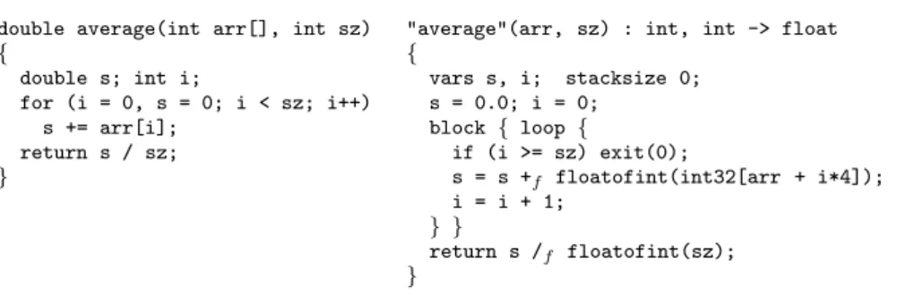
Fig. 5 An example of a Cminor function (right) and the corresponding C code (left).
current stack data block before invoking the function. This enables tail recursion to execute in constant stack space.
Besides the familiar sequence s1; s2and if/then/else constructs, control flow can
be expressed either in an unstructured way using goto and labeled statements or in a structured way using infinite loops and the block/exit construct. exit(n) where n ≥ 0 branches to the end of the (n + 1)th enclosing block construct. The switch(a) {tbl } construct matches the integer value of a against the cases listed in tbl and performs the corresponding exit. Appropriate nesting of a switch within several block constructs suffices to express C-like structured switch statements with fall-through behavior. Internal functions: F ::= { sig = sig; function signature
params= ~id; parameters vars= ~id ; local variables
stacksize= n; size of stack data in bytes
body= s } function body
In addition to a parameter list, local variable declarations and a function body (a statement), a function definition comprises a type signature sig and a declaration of how many bytes of stack-allocated data it needs. A Cminor local variable does not reside in memory, and its address cannot be taken. However, the Cminor producer can explicitly stack-allocate some data (such as, in C, arrays and scalar variables whose addresses are taken). A fresh memory block of size F.stacksize is allocated each time F is invoked and automatically freed when it returns. The addrstack(δ) nullary operator returns a pointer within this block at byte offset δ.
Figure 5 shows a simple C function and the corresponding Cminor function, using an ad-hoc concrete syntax for Cminor. Both functions compute the average value of an array of integers, using float arithmetic. Note the explicit address computation int32[tbl + i*4]to access element i of the array, as well as the explicit floatofint conversions. The for loop is expressed as an infinite loop wrapped in a block, so that exit(0) in the Cminor code behaves like the break statement in C.
4.2 Dynamic semantics
The dynamic semantics of Cminor is defined using a combination of natural seman-tics for the evaluation of expressions and a labeled transition system in the style of section 3.5 for the execution of statements and functions.
E(id) = ⌊v⌋ G, σ, E, M⊢ id ⇒ v eval constant(G, σ, cst) = ⌊v⌋ G, σ, E, M⊢ cst ⇒ v G, σ, E, M⊢ a1⇒ v1 eval unop(op1, v1) = ⌊v⌋ G, σ, E, M⊢ op1(a1) ⇒ v G, σ, E, M⊢ a1⇒ v1 G, σ, E, M⊢ a2⇒ v2 eval binop(op2, v1, v2) = ⌊v⌋ G, σ, E, M⊢ op2(a1, a2) ⇒ v G, σ, E, M⊢ a1⇒ ptr(b, δ) load(M, κ, b, δ) = ⌊v⌋ G, σ, E, M⊢ κ[a1] ⇒ v G, σ, E, M⊢ a1⇒ v1 istrue(v1) G, σ, E, M⊢ a2⇒ v2 G, σ, E, M⊢ (a1 ? a2: a3) ⇒ v2 G, σ, E, M⊢ a1⇒ v1 isfalse(v1) G, σ, E, M⊢ a3⇒ v3 G, σ, E, M⊢ (a1 ? a2: a3) ⇒ v3 G, σ, E, M⊢ ǫ : ǫ G, σ, E, M⊢ a ⇒ v G, σ, E, M⊢ ~a ⇒ ~v G, σ, E, M⊢ a.~a ⇒ v.~v Evaluation of constants:
eval constant(G, σ, i) = ⌊int(i)⌋ eval constant(G, σ, f ) = ⌊float(f )⌋ eval constant(G, σ, addrsymbol(id )) = symbol(G, id)
eval constant(G, σ, addrstack(δ)) = ⌊ptr(σ, δ)⌋ Evaluation of unary operators (selected cases):
eval unop(negf, float(f )) = ⌊float(−f )⌋ eval unop(notbool, v) = ⌊int(0)⌋ if istrue(v) eval unop(notbool, v) = ⌊int(1)⌋ if isfalse(v) Evaluation of binary operators (selected cases):
eval binop(add, int(n1), int(n2)) = ⌊int(n1+ n2)⌋ (mod 232)
eval binop(add, ptr(b, δ), int(n)) = ⌊ptr(b, δ + n)⌋ (mod 232
)
eval binop(addf, float(f1), float(f2)) = ⌊float(f1+ f2)⌋
Truth values:
istrue(v) def= vis ptr(b, δ) or int(n) with n 6= 0
isfalse(v) def= vis int(0)
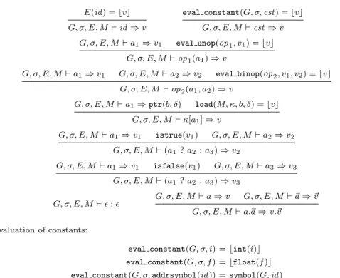
Fig. 6 Natural semantics for Cminor expressions.
4.2.1 Evaluation of expressions
Figure 6 defines the big-step evaluation of expressions as the judgment G, σ, E, M ⊢ a ⇒ v, where a is the expression to evaluate, v its value, σ the stack data block, E an environment mapping local variables to values, and M the current memory state. The evaluation rules are straightforward. Most of the semantics is in the definition of the auxiliary functions eval_constant, eval_unop and eval_binop, for which some
representative cases are shown. These functions can return ∅, causing the expression to be undefined, if for instance an argument of an operator is undef or of the wrong type. Some operators (add, sub and cmp) operate both on integers and on pointers.
4.2.2 Execution of statements and functions
The labeled transition system that defines the small-step semantics for statements and function invocations follows the general pattern shown in sections 3.5 and 3.6. Program states have the following shape:
Program states: S ::= S(F, s, k, σ, E, M ) regular state
| C(Fd , ~v, k, M ) call state
| R(v, k, M ) return state
Continuations: k ::= stop initial continuation
| s; k continue with s, then do as k
| endblock(k) leave a block, then do as k
| returnto(id?, F, σ, E, k) return to caller
Regular states S carry the currently-executing function F , the statement under con-sideration s, the block identifier for the current stack data σ, and the values E of local variables.
Following a proposal by Appel and Blazy [3], we use continuation terms k to encode both the call stack and the program point within F where the statement s under consideration resides. A continuation k records what needs to be done once s reduces to skip, exit or return. The returnto parts of k represent the call stack: they record the local states of the calling functions. The top part of k up to the first returnto corresponds to an execution context for s, represented inside-out in the style of a zipper [45]. For example, the continuation s; endblock(. . .) corresponds to the context block{ [ ]; s }.
Figures 7 and 8 list the rules defining the transition relation G ⊢ S → St ′
. The rules in figure 7 address transitions within the currently-executing function. They are roughly of three kinds:
– Execution of an atomic computation step. For example, the rule for assignments transitions from id = a to skip.
– Focusing on the active part of the current statement. For example, the rule for sequences transitions from (s1; s2) with continuation k to s1 with continuation
s2; k.
– Resuming a continuation that was set apart in the continuation. For instance, one of the rules for skip transitions from skip with continuation s; k to s with continuation k.
Two auxiliary functions over continuations are defined: callcont(k) discards the local context part of the continuation k, and findlabel(lbl, s, k) returns a pair (s′
, k′
) of the leftmost sub-statement of s labeled lbl and of a continuation k′
that extends k with the context surrounding s′
. The combination of these two functions in the rule for goto suffices to implement the branching behavior of goto statements.
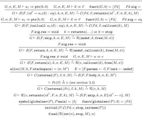
Figure 8 lists the transitions involving call states and return states, and defines initial states and final states. The definitions follow the general pattern depicted in fig-ure 3. In particular, initial states are call states to the “main” function of the program, with no arguments and the stop continuation; symmetrically, final states are return
G⊢ S(F, skip, (s; k), σ, E, M )→ S(F, s, k, σ, E, M )ǫ
G⊢ S(F, skip, endblock(k), σ, E, M )→ S(F, skip, k, σ, E, M )ǫ
G, σ, E, M⊢ a ⇒ v
G⊢ S(F, (id = a), k, σ, E, M )→ S(F, skip, k, σ, E{id ← v}, M )ǫ
G, σ, E, M⊢ a1⇒ ptr(b, δ) G, σ, E, M⊢ a2⇒ v store(M, κ, b, δ, v) = ⌊M′⌋ G⊢ S(F, (κ[a1] = [a2]), k, σ, E, M )→ S(F, skip, k, σ, E, Mǫ ′) G⊢ S(F, (s1; s2), k, σ, E, M ) ǫ → S(F, s1,(s2; k), σ, E, M ) G, σ, E, M⊢ a ⇒ v istrue(v) G⊢ S(F, (if(a){s1} else {s2}), k, σ, E, M ) ǫ → S(F, s1, k, σ, E, M) G, σ, E, M⊢ a ⇒ v isfalse(v) G⊢ S(F, (if(a){s1} else {s2}), k, σ, E, M ) ǫ → S(F, s2, k, σ, E, M) G⊢ S(F, loop{s}, k, σ, E, M )→ S(F, s, (loop{s}; k), σ, E, M )ǫ G⊢ S(F, block{s}, k, σ, E, M )→ S(F, s, endblock(k), σ, E, M )ǫ G⊢ S(F, exit(n), (s; k), σ, E, M )→ S(F, exit(n), k, σ, E, M )ǫ
G⊢ S(F, exit(0), endblock(k), σ, E, M )→ S(F, skip, k, σ, E, M )ǫ
G⊢ S(F, exit(n + 1), endblock(k), σ, E, M )→ S(F, exit(n), k, σ, E, M )ǫ
G, σ, E, M⊢ a ⇒ int(n)
G⊢ S(F, (switch(a){tbl }), k, σ, E, M )→ S(F, exit(tbl(n)), k, σ, E, M )ǫ
G⊢ S(F, (lbl : s), k, σ, E, M )→ S(F, s, k, σ, E, M )ǫ
findlabel(lbl , F.body, callcont(k)) = ⌊s′, k′⌋
G⊢ S(F, goto lbl , k, σ, E, M )→ S(F, sǫ ′, k′, σ, E, M)
callcont(s; k) = callcont(k) callcont(endblock(k)) = callcont(k)
callcont(k) = k otherwise
findlabel(lbl , (s1; s2), k) = findlabel(lbl, s1,(s2; k)) if not ∅;
findlabel(lbl , s2, k) otherwise
findlabel(lbl , if(a){s1} else {s2}, k) = findlabel(lbl, s1, k) if not ∅;
findlabel(lbl , s2, k) otherwise
findlabel(lbl , loop{s}, k) = findlabel(lbl , s, (loop{s}; k)) findlabel(lbl , block{s}, k) = findlabel(lbl , s, endblock(k))
findlabel(lbl , (lbl : s), k) = ⌊s, k⌋
findlabel(lbl , (lbl′: s), k) = findlabel(lbl , s, k) if lbl′6= lbl
Fig. 7 Transition semantics for Cminor, part 1: statements.
states with the stop continuation. The rules for function calls require that the signa-ture of the called function matches exactly the signasigna-ture annotating the call; otherwise execution gets stuck. A similar requirement exists in the C standard and is essential to support signature-dependent calling conventions later in the compiler. Taking again a leaf from the C standard, functions are allowed to terminate by return without an argument or by falling through their bodies only if their return signatures are void.
G, σ, E, M⊢ a1⇒ ptr(b, 0) G, σ, E, M⊢ ~a ⇒ ~v funct(G, b) = ⌊Fd ⌋ Fd .sig= sig G⊢ S(F, (id? = a1(~a) : sig), k, σ, E, M ) ǫ → C(Fd, ~v, returnto(id? , F, σ, E, k), M )
G, σ, E, M⊢ a1⇒ ptr(b, 0) G, σ, E, M⊢ ~a ⇒ ~v funct(G, b) = ⌊Fd ⌋ Fd .sig= sig
G⊢ S(F, (tailcall a1(~a) : sig), k, σ, E, M )
ǫ
→ C(Fd , ~v, callcont(k), M )
F.sig.res= void k= returnto(. . .) or k = stop
G⊢ S(F, skip, k, σ, E, M )→ R(undef, k, free(M, σ))ǫ
F.sig.res= void
G⊢ S(F, return, k, σ, E, M )→ R(undef, callcont(k), free(M, σ))ǫ
F.sig.res6= void G, σ, E, M⊢ a ⇒ v
G⊢ S(F, return(a), k, σ, E, M )→ R(v, callcont(k), free(M, σ))ǫ
alloc(M, 0, F.stackspace) = (σ, M′) E= [F.params ← ~v; F.vars ← undef]
G⊢ C(internal(F ), ~v, k, M )→ S(F, F.body, k, σ, E, Mǫ ′)
⊢ Fe(~v)⇒ v (see section 3.4)t
G⊢ C(external(Fe), ~v, k, M )→ R(v, k, M )t
G⊢ R(v, returnto(id?, F, σ, E, k), M )→ S(F, skip, k, σ, E{idǫ ?← v}, M )
symbol(globalenv(P ), P.main) = ⌊b⌋ funct(globalenv(P ), b) = ⌊Fd⌋
initial(P, C(Fd , ǫ, stop, initmem(P ))) final(R(int(n), stop, M ), n)
Fig. 8 Transition semantics for Cminor, part 2: functions, initial states, final states.
4.2.3 Alternate natural semantics for statements and functions
For some applications, it is convenient to have an alternate natural (big-step) opera-tional semantics for Cminor. We have developed such a semantics for the fragment of Cminorthat excludes goto and labeled statements. The big-step judgments for termi-nating executions have the following form:
G, σ ⊢ s, E, M⇒ out, Et ′ , M′ (statements) G ⊢ Fd (~v), M⇒ v, Mt ′ (function calls) E′ and M′
are the local environment and the memory state at the end of the execution; t is the trace of events generated during execution. Following Huisman and Jacobs [46], the outcome out indicates how the statement s terminated: either normally by running to completion (out = Normal); or prematurely by executing an exit statement (out = Exit(n)), return statement (out = Return(v?) where v?is the value of the optional argument to return), or tailcall statement (out = Tailreturn(v)). Additionally, we followed the coinductive approach to natural semantics of Leroy and Grall [60] to define (coinductively) big-step judgments for diverging executions, of the form
G, σ ⊢ s, E, M⇒ ∞T (diverging statements) G ⊢ Fd (~v), M⇒ ∞ (diverging function calls)T The definitions of these judgments can be found in the Coq development.
Theorem 5 The natural semantics of Cminor is correct with respect to its transition
semantics:
1. If G ⊢ Fd (~v), M⇒ v, Mt ′
, then G ⊢ C(Fd , ~v, k, M )→t∗
R(v, k, M′
) for all
continu-ations k such that k = callcont(k).
2. If G ⊢ Fd (~v), M⇒ ∞, then G ⊢ C(Fd , ~v, k, M )T → ∞ for all continuations k.T
4.3 Static typing
Cminoris equipped with a trivial type system having only two types: int and float. (Pointers have static type int.) Function definitions and function calls are annotated with signatures sig giving the number and types of arguments, along with optional result types. All operators are monomorphic; therefore, the types of local variables can be inferred from their uses and are not declared.
The primary purpose of this trivial type system is to facilitate later transformations (see sections 8 and 12); for this purpose, all intermediate languages of Compcert are equipped with similar int-or-float type systems. By themselves, these type systems are too weak to give type soundness properties (absence of run-time type errors). For example, performing an integer addition of two pointers or two undef values is statically well-typed but causes the program to get stuck. Likewise, calling a function whose signature differs from that given at the call site is a run-time error, undetected by the type system; its semantics are not defined and the compiler can (and does) generate incorrect code for this call. It is the responsibility of the Cminor producer to avoid these situations, e.g. by using a richer type system. Nevertheless, the Cminor type system enjoys a type preservation property: values of static type int are always integers, pointers or undef, and values of static type float are always floating-point numbers or undef. This weak soundness property plays a role in the correctness proofs of section 12.3.
5 Instruction selection
The first compilation pass of Compcert rewrites expressions to exploit the combined arithmetic operations and addressing modes of the target processor. To take better advantage of the processor’s capabilities, reassociation of integer additions and multi-plications is also performed, as well as a small amount of constant propagation.
5.1 The target language: CminorSel
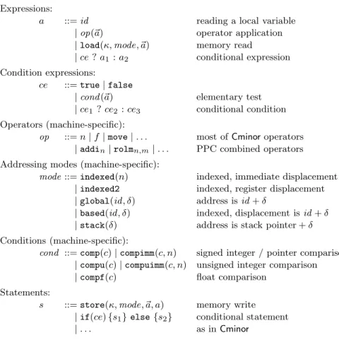
The target language for this pass is CminorSel, a variant of Cminor that uses a dif-ferent, processor-specific set of operators. Additionally, a syntactic class of condition expressions ce (expressions used only for their truth values) is introduced.
Expressions:
a ::= id reading a local variable
| op(~a) operator application
| load(κ, mode, ~a) memory read
| ce ? a1: a2 conditional expression
Condition expressions:
ce ::= true | false
| cond (~a) elementary test
| ce1? ce2: ce3 conditional condition
Operators (machine-specific):
op ::= n | f | move | . . . most of Cminor operators
| addin| rolmn,m| . . . PPC combined operators
Addressing modes (machine-specific):
mode ::= indexed(n) indexed, immediate displacement
| indexed2 indexed, register displacement
| global(id, δ) address is id + δ
| based(id, δ) indexed, displacement is id + δ
| stack(δ) address is stack pointer + δ
Conditions (machine-specific):
cond ::= comp(c) | compimm(c, n) signed integer / pointer comparison | compu(c) | compuimm(c, n) unsigned integer comparison
| compf(c) float comparison
Statements:
s ::= store(κ, mode, ~a, a) memory write
| if(ce) {s1} else {s2} conditional statement
| . . . as in Cminor
For the PowerPC, the machine-specific operators op include all Cminor nullary, unary and binary operators except notint, mod and modu (these need to be synthe-sized from other operators) and adds immediate forms of many integer operators, as well as a number of combined operators such as not-or, not-and, and rotate-and-mask. (rolmn,m is a left rotation by n bits followed by a logical “and” with m.) A
mem-ory load or store now carries an addressing mode mode and a list of expressions ~a, from which the address being addressed is computed. Finally, conditional expressions and conditional statements now take condition expressions ce as arguments instead of normal expressions a.
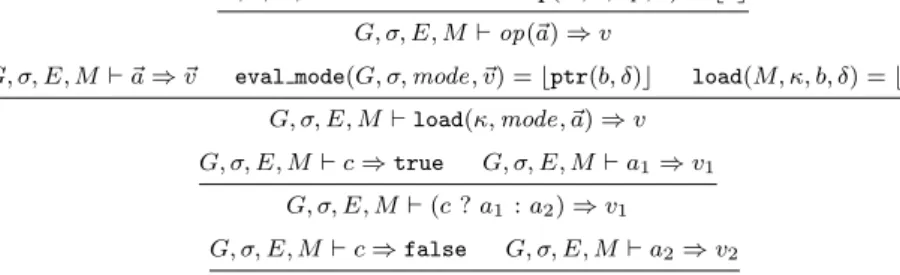
The dynamic semantics of CminorSel resembles that of Cminor, with the addition of a new evaluation judgment for condition expressions G, σ, E, M ⊢ ce ⇒ (false | true). Figure 9 shows the main differences with respect to the Cminor semantics.
5.2 The code transformation
Instruction selection is performed by a bottom-up rewriting of expressions. For each Cminor operator op, we define a “smart constructor” function written op that takes CminorSelexpressions as arguments, performs shallow pattern-matching over them to recognize combined or immediate operations, and returns the corresponding CminorSel