Combining Adaptive and Designed Statistical
Experimentation: Process Improvement, Data
Classification, Experimental Optimization, and Model
Building
by
Chad Ryan Foster
B.S., Colorado School of Mines (1998)
M.S., University of Texas at Austin (2000)
Submitted to the Department of Mechanical Engineering
in partial fulfillment of the requirements for the degree of
Doctor of Philosophy
at the
MASSACHUSETTS INSTITUTE OF TECHNOLOGY
June 2009
c
Massachusetts Institute of Technology 2009. All rights reserved.
Author . . . .
Department of Mechanical Engineering
March 11, 2009
Certified by . . . .
Daniel D. Frey
Associate Professor
Thesis Supervisor
Accepted by . . . .
David E. Hardt
Chairman, Department Committee on Graduate Theses
i
Combining Adaptive and Designed Statistical Experimentation:
Process Improvement, Data Classification, Experimental
Optimization, and Model Building
by
Chad Ryan Foster
Submitted to the Department of Mechanical Engineering on March 11, 2009, in partial fulfillment of the
requirements for the degree of Doctor of Philosophy
Abstract
Research interest in the use of adaptive experimentation has returned recently. This his-toric technique adapts and learns from each experimental run but requires quick runs and large effects. The basis of this renewed interest is to improve experimental response and it is supported by fast, deterministic computer experiments and better post-experiment data analysis. The unifying concept of this thesis is to present and evaluate new ways of us-ing adaptive experimentation combined with the traditional statistical experiment. The first application uses an adaptive experiment as a preliminary step to a more traditional experimental design. This provides experimental redundancy as well as greater model ro-bustness. The number of extra runs is minimal because some are common and yet both methods provide estimates of the best setting. The second use of adaptive experimentation is in evolutionary operation. During regular system operation small, nearly unnoticeable, variable changes can be used to improve production dynamically. If these small changes follow an adaptive procedure there is high likelihood of improvement and integrating into the larger process development. Outside of the experimentation framework the adaptive procedure is shown to combine with other procedures and yield benefit. Two examples used here are an unconstrained numerical optimization procedure as well as classification parameter selection.
The final area of new application is to create models that are a combination of an adap-tive experiment with a traditional statistical experiment. Two distinct areas are examined, first, the use of the adaptive experiment to determine the covariance structure, and second, the direct incorporation of both data sets in an augmented model. Both of these applications are Bayesian with a heavy reliance on numerical computation and simulation to determine
the combined model. The two experiments investigated could be performed on the same physical or analytical model but are also extended to situations with different fidelity mod-els. The potential for including non-analytical, even human, models is also discussed.
The evaluative portion of this thesis begins with an analytic foundation that outlines the usefulness as well as the limitations of the procedure. This is followed by a demonstration using a simulated model and finally specific examples are drawn from the literature and reworked using the method.
The utility of the final result is to provide a foundation to integrate adaptive experi-mentation with traditional designed experiments. Giving industrial practitioners a solid background and demonstrated foundation should help to codify this integration. The final procedures represent a minimal departure from current practice but represent significant modeling and analysis improvement.
Thesis Supervisor: Daniel D. Frey Title: Associate Professor
Acknowledgements
This work was possible only with the guidance of my many mentors in and around MIT in-cluding Dan Frey, Maria Yang, Warren Seering, Chris Magee, Alex Slocum, David Rumpf, and Tony Patera, plus the lively discussion and interaction of my fellow researchers Nan-dan Sudarsanam, Xiang Li, Jagmeet Singh, Sidharth Rupani, Yiben Lin, Rajesh Jugulum, Hungjen Wang, Ben Powers, Konstantinos Katsikopoulos, Lawrence Neeley, Helen Tsai, and Jonathan Evans, as well as international correspondence with Monica Altamirano, Leslie Zachariah, Catherine Chiong-Meza, Michiel Houwing, Paulien Herder, and Pepijn Dejong and finally the financial support of MIT, NSF, MIT Pappalardo Fellowship, Cum-mins, GE, Landis, and, of course, the support and encouragement of Elise and the rest of my family.
Table of Contents
1 Introduction 1
Bibliography . . . 8
2 Experimental Background 11 2.1 Early Experimental Developments . . . 11
2.1.1 Higher Order Models . . . 16
2.2 Adaptive Designs . . . 18
2.3 Background for One-Factor-at-a-Time (OFAT) . . . 20
2.4 Adaptive One-Factor-at-a-Time (aOFAT) . . . 22
2.5 aOFAT Opportunities . . . 26
2.6 Prediction Sum of Squares (PRESS) . . . 29
2.7 Empirical Bayesian Statistics . . . 31
2.8 Gaussian Process (GP) . . . 32
2.9 Hierarchical Probability Model . . . 33
2.10 Opportunities . . . 35 Bibliography . . . 37 3 Reusing Runs 41 3.1 Introduction . . . 41 3.2 Background . . . 42 3.3 Initialization . . . 43
3.4 Reusing aOFAT runs in a Fractional Factorial . . . 44
3.5 D-Optimal Augmentation . . . 47
3.6 Maximum Value Choice . . . 49
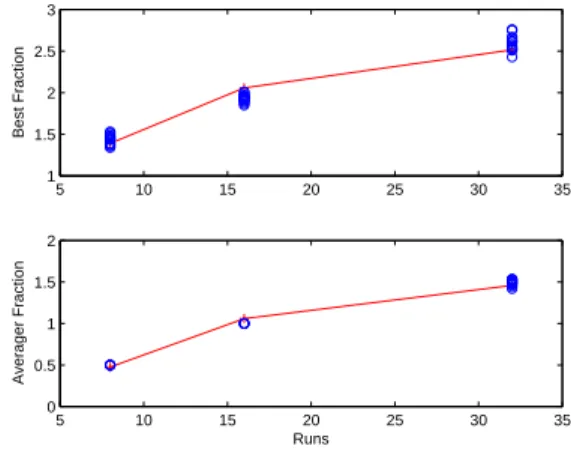
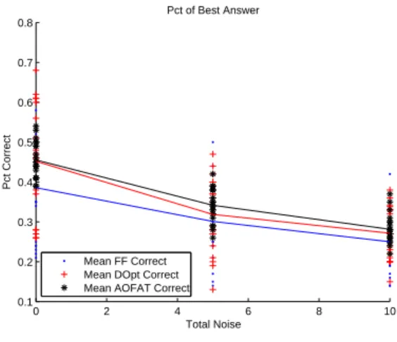
3.7 Sheet Metal Spinning . . . 51
3.8 Using Both Models . . . 53 v
3.9 Conclusion . . . 53 Bibliography . . . 55 4 Evolutionary Operation 57 4.1 Introduction . . . 57 4.2 Background . . . 58 4.3 Other Models . . . 59 4.4 Run Size . . . 61 4.5 Comparison to Optimization . . . 64 4.6 Empirical Improvement . . . 65 4.7 Additional Runs . . . 69 4.8 Conclusion . . . 73 Bibliography . . . 75
5 Sequential Simplex Initialization 77 5.1 Introduction . . . 77
5.2 Background . . . 78
5.3 Initializing the Simplex . . . 79
5.4 Proposed Improvement . . . 80
5.5 Improvement Considerations . . . 82
5.6 Test Cases . . . 84
5.7 Conclusion . . . 86
Bibliography . . . 88
6 Mahalanobis Taguchi Classification System 91 6.1 Introduction . . . 92
6.1.1 Description of Experimentation Methodology . . . 95
6.1.2 Image Classification System . . . 96
6.2 Feature Extraction Using Wavelets . . . 97
6.3 Comparing Results of the Different Methods . . . 100
6.4 Conclusion . . . 102
Bibliography . . . 103
7 aOFAT Integrated Model Improvement 105 7.1 Introduction . . . 105
TABLE OF CONTENTS vii
7.2 Background . . . 106
7.3 Procedure . . . 108
7.4 Analysis . . . 112
7.5 Results . . . 119
7.5.1 Hierarchical Probability Model (HPM) . . . 120
7.5.2 Analytic Example . . . 124
7.5.3 Wet Clutch Experiment . . . 126
7.6 Conclusion . . . 127
Bibliography . . . 129
8 Combining Data 131 8.1 Background . . . 132
8.2 Process . . . 133
8.3 Hierarchical Two-Phase Gaussian Process Model . . . 136
8.4 Simulation Procedure . . . 145 8.5 Convergence . . . 148 8.6 Krigifier (Trosset, 1999) . . . 154 8.7 Results . . . 155 8.8 Conclusion . . . 159 Bibliography . . . 160 9 Conclusions 163 9.1 Future Work . . . 166 9.2 Summary . . . 167 Bibliography . . . 168
A Adaptive Human Experimentation 169 A.1 Layout . . . 170
A.2 Background . . . 171
A.3 Potential Research . . . 173
A.4 Work . . . 174
A.5 Previous Work . . . 176
A.6 Potential Contribution . . . 177
B Replacing Human Classifiers: A Bagged Classification System 181 B.1 Introduction . . . 182 B.2 Classifier Approach . . . 183 B.3 Combining Classifiers . . . 188 B.4 Conclusion . . . 192 Bibliography . . . 194
List of Figures
2-1 Ronald A. Fisher . . . 12
2-2 William S. Gosset . . . 12
3-1 Fractional Factorial Run Reuse . . . 45
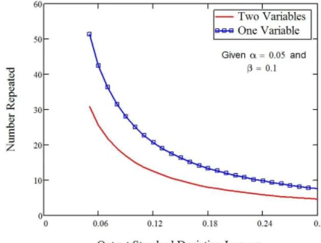
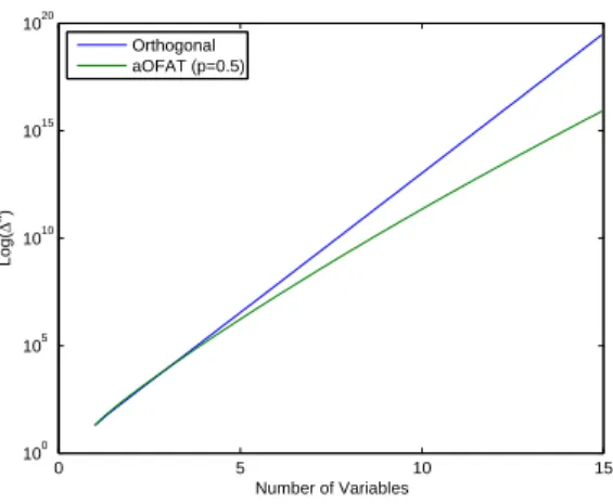
3-2 Asymptotic Runs Function . . . 47
3-3 D-Optimal Run Reuse . . . 49
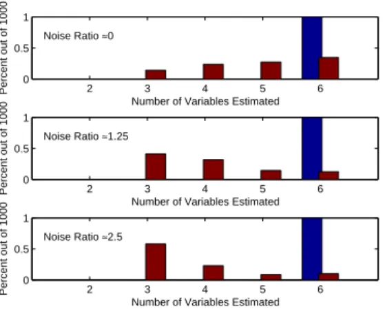
3-4 HPM percent correct compared with noise . . . 51
3-5 Sheet metal spinning repeated runs . . . 52
3-6 Percent of best answer in sheet metal spinning example . . . 52
4-1 EVOP Terms Repeated . . . 62
4-2 Repeated Runs . . . 67
4-3 Single Variable Probability Incorrect . . . 68
4-4 Single Variable Loss Standard Deviation . . . 69
4-5 Response with noise variation, aOFAT is blue on the left and Fractional Factorial red on the right. . . 71
4-6 Number of modeled variables, aOFAT is blue on the left and the Fractional Factorial red on the right. . . 72
5-1 Distance to Centroid . . . 82
5-2 Volume of Simplex . . . 84
5-3 Centroid Distance Comparison . . . 85
6-1 Steps in MTS . . . 94
6-2 Fine art images before and after application of noise . . . 98
6-3 The Mona Lisa reconstructed from its wavelet transform after all but the N X N coarsest levels of scale have been discarded . . . 99
6-4 Results of the three search methods for the image classification . . . 101
7-1 aOFAT Percentage Improvement . . . 109
7-2 Expected Improvement Comparison . . . 111
7-3 Additional Variable Slope . . . 112
7-4 Hierarchical Probability Model (HPM) Comparison . . . 122
7-5 HPM Large Experiment . . . 122
7-6 HPM Weighted Large Experiment . . . 123
7-7 HPM Same Second Experiment Size . . . 123
7-8 Wu and Hamada (2000) Analytical Experiment . . . 125
7-9 Wet Clutch Example . . . 126
7-10 Wet Clutch Comparison . . . 127
8-1 MCMC Convergence . . . 149
8-2 MCMC Convergence Continued . . . 150
8-3 MCMC Convergence ˆR . . . 152
8-4 MCMC Convergence ˆRQ . . . 153
8-5 Prediction error . . . 157
8-6 Prediction error for run maximum only . . . 157
B-1 Four Example Zip Codes. Five number images from the 10,000 possible images . . . 184
B-2 Variables Per Tree. Given 5, 10, 15, and 20 variables for each tree the accuracy in percent correct is compared with the logistic probability in the top panel. The bottom panel shows the percent of data less than the logistic probability . . . 185
B-3 Confidence Estimate on Training Data. The relationship between the error on the training data and the logistic probability is given in the top panel. The percentage of the data less than the logistic probability is given in the bottom panel. . . 187
B-4 Different Human Classifiers. The relationship between the logistic proba-bility and the accuracy for all 10,000 images is given in the top panel for three different classifiers and their combined estimate. The bottom panel shows the percentage of the population less than the logistic probability . . 189
LIST OF FIGURES xi
B-5 Percentage Rework. This plot is based on a marginal probability for the logistic parameter of 0.85 and three judges. The individual percentage
re-duction pr is on the horizontal axis and the percentage rework is on the
List of Tables
2.1 Plackett-Burman Generating Row . . . 18
3.1 aOFAT Reuse Comparison . . . 46
5.1 Unconstrained Optimization Test Functions . . . 89
Chapter 1
Introduction
Many experimental situations require a setup, tuning, or a variable importance decision be-fore running a designed experiment. If this other procedure is run as an adaptive experiment there can be additional benefit to the subsequent designed experiment. The adaptive experi-ment of focus is the adaptive-One-Factor-at-a-Time (aOFAT) experiexperi-ment described in Frey et al. (2003), to be combined with a number of different statistically designed experiments including fractional factorial, Box-Behnken, Plackett-Burman, and D-Optimal as well as other procedures including evolutionary operation, article classification, and unconstrained optimization. The hypothesis is that there is an appropriate and beneficial place within designed experimentation to combine an adaptive experiment with a traditional statistical experiment.
Design-of-experiments (DOE) is a frequently used tool to understand and improve a system. The experimental technique began as support for long-term agricultural projects that allowed the development of methods such as blocking, randomization, replication, and fractional factorial analysis (Box et al., 2005). Many of these practices are considered fundamental to good experimentation, and are widely used today. The next advancement
to experimentation were achieved by industrial practitioners. In the chemical and man-ufacturing industries experiments ran more quickly, but were still expensive. Sequential experimentation specifically designed for regression analysis became the standard. The ex-periment was tied to a particular underlying physical model and could accurately estimate the required model parameters with minumum excessive runs. In current experimentation research design parameters are separated from noise parameters to allow robustness tun-ing, with the most popular technique being crossed arrays (Wu and Hamada, 2000). These methods rely on a single design paradigm, the statistical experiment. The previous method of changing a one factor at a time (OFAT) (Daniel, 1973) has been discounted as lacking the statistical power and requiring too many runs (Wu and Hamada, 2000). The advantages of learning from each run and approaching a maximum quickly are under appreciated and over criticized. This adaptive approach is also easy to explain and implement and does not require an extensive statistical background.
The literature on experimentation (Wu and Hamada, 2000; Montgomery, 1996; Box et al., 2005) is primarily from a statistical viewpoint and differing in paradigm from the previous one-factor approach, as Kuhn (1996) would say, the discussions between the two options may be incommensurable. The arguments for the statistical approach are based on a language and perspective that does not exist with the one-factor methodology. Even with a preponderance of evidence in support of the one-factor approach in certain situations, yielding slightly is tantamount to questioning the foundation for a statistical approach. The suggestion forwarded in this work is partially that an opportunity exists to bridge the paradigms of one-factor and statistical experiments. It is not to belittle the advancement of statistical experiments but to expand the framework to consider the system of application. A parallel can be drawn to Newtonian and relativistic physics. While it is accepted that for high speed and short time applications the Einstein view is more correct, for the majority of
3
earth bound physics the Newtonian approach is more useful. Einstein (1919) also suggests that his theory does not supersede Newtonian physics and finding accessible situations to measure any difference is difficult. From a practical standpoint, accepting the validity of Einstein does not reduce the ubiquitous utility of Newtonian physics in daily engineering activities. The same approach could be taken in experimentation. While acknowledging the validity of statistical experimentation there are situations where one-factor methodologies are more practical. Taking this openness even further there are opportunities to benefit from both a one-factor design as well as a statistical experiment. The analogy would be initial predictions using Newtonian physics to be later refined with relativistic calculations. For many instruments and situations the initial method would be sufficient but the confirmation and refinement using a relativistic approach would support the results.
Although the statistical and adaptive approaches are traditionally used in different sit-uations this work will present opportunities to combine the results from both types of ex-periments into a complete testing framework. This combination is challenging to accept by both the academic as well as the industrial community. The academics question the pragmatic utility while most practitioners are unwilling to challenge the foundation of their six-sigma training. Although it may be impossible to bridge the incommensurate points of view, this work is an attempt to present some specific examples that demonstrate the utility of using both methodologies.
The first situation of interest is reusing runs from a prior adaptive experiment. By reusing runs the intent is to increase the number of common runs between the two exper-iments. The adaptive experiment cannot be preplanned and so the potential reuse in the subsequent experiment is stochastic. The procedure investigated begins with an aOFAT experiment. The first follow-up experiment is a traditional fractional factorial design. The number of runs reused is dependent on the fraction used, the number of variables, and size
of fraction. This number asymptotes to approximately twenty percent of the total adaptive runs. This run reuse is demonstrated on a number of actual experiments as well as surrogate experiments. If the follow-up experiment is more flexible in design, one option investigated was the non-balanced D-optimal design. As suggested in Wu and Hamada (2000), a fully orthogonal non-balanced D-optimal design is a good alternative to a fractional factorial. This change dramatically improves run reuse to all but one run, although it requires design planning after the initial aOFAT is complete. In addition to simulating the results of this improvement the independence of the two resultant maximum settings is demonstrated. Running an adaptive experiment before a statistical experiment creates an opportunity for run reuse while providing an independent maximum setting estimates.
This adaptive approach could also be used on the manufacturing floor. The method of evolutionary operation (EVOP) is revisited with a focus on utilizing adaptive experi-mentation. The alignment of this continuous improvement technique with the sequential maximization nature of an aOFAT provides a positive pairing. The use of these adaptive procedures was discussed by Box and Draper (1969) to the conclusion that the methodology was na ive. This conclusion is challenged here by investigating actual system responses, and showing a place for sequential adaptive experiments. Instead of using small fractional factorial experiments, repeated single steps in an adaptive procedure is shown to be more robust to initial and subsequent variable selection. Because of the stochastic nature of the repeated procedure a modified Gibbs sampler is introduced to minimize the additional runs while converging to a better variable setting. An offshoot of this procedure is the use of an adaptive experiment in computational function maximization.
The modified sequential simplex procedure was originally developed for evolutionary operation (Spendley et al., 1962). This rank-based geometric procedure was used fre-quently in the 1970’s and 1980’s although it languished in the 1990’s for more complex
5
derivative-based methods. More recently it has returned to popularity with the increased use of computer simulations. As a robust method it is able to handle discontinuities and noise at the cost of more function evaluations. There are implementations of the simplex in most numerical programs for unconstrained optimization. The typical initial setup is based on changing one variable at a time (Press et al., 2007). This is improved by adding an adaptive element and performing an aOFAT for the initialization. The aOFAT procedure is modified to align the geometric center of the starting points to that of the non-adaptive method to permit equivalent comparisons. The adaptive procedure improves the overall convergence and reduces the number of function evaluations. Combining the adaptive pro-cedure with the simplex starts the geometric propro-cedure towards the maximum gradient for improved convergence. The benefit of this change is demonstrated on a test suite for nu-merical optimization (Mor´e et al., 1981).
Outside of the optimization another issue addressed here is variable selection. Using the Mahalanobis-Taguchi Strategy (MTS) from Taguchi and Jugulum (2002), data classifi-cation is based on a statistical distance. One hurdle to using this system is in selecting the best variables for classification. Traditionally orthogonal arrays are used to select a subset of variables. This method can be improved by using an aOFAT experiment combined with the Mahalanobis distance. This procedure is specifically applied to an image classification system where the variables of interest are the coefficients of a wavelet transform. In this case the addition of variables adds to the computational load of the classification system reducing its performance. It is important to add the minimum number of variables while maximizing their usefulness. The superior peroformance of the aOFAT combined approach is demonstrated and has been published in Foster et al. (2009).
In addition to dual results and as a starting procedure, aOFAT can be used as one ex-periment that combines the results into a single model. Combining two different types of
data was approached in a Bayesian framework. The use of a correlated gaussian random variable to make a posterior prediction has been used successfully by Joseph (2006). Part of this methodology is to use a correlation matrix for the input variables. Instead of using a larger experiment the information was divided between an early aOFAT experiment to cre-ate the correlation matrix followed by a highly aliased Plackett-Burman design (Plackett and Burman, 1946). The goal of this aspect of the work is to combine the relative strengths of both the aOFAT and traditional experimental procedures. The aOFAT can be used to create a variable ranking while the aliased design is able to efficiently define the model. A procedure to define the correlation matrix is created that benefits from published data regularities (Wu and Hamada, 2000) and variable distribution (Li and Frey, 2005). This methods performance is equivalent to using an uninformed correlation matrix and a larger experimental design with equal total runs. The procedure is demonstrated on a number of published examples as well as surrogate functions.
The last aspect of combined model building is to use experiments of different accuracy such as Qian and Wu (2008). Combining computational and physical experiments is one example of these different accuracies. The use of adaptive experiments uses a minimum number of runs while increasing the likelihood of having points near the maximum. A new method of calculating convergence is presented as well as a procedure to maximize each simulated markov chain. The result is a procedure that provides a good model using both data types that is more accurate at the maximum values.
The ultimate goal of this work is to create a foundation for the integration of adaptive experimentation into statistical experiments. Simple techniques are presented for using setup runs and getting benefit from those runs. This continues to manufacturing where evolutionary operation (EVOP) can be improved and simplified with adaptive experiments. A numerical maximization procedure is improved through a better starting approach, and
7
a classification procedure is shown to benefit from an adaptive parameter selection tech-nique. The final area focused on using data from an adaptive experiment and a traditional experiment to build a single model. First, the covariance estimation was improved to yield more accurate and smaller models with the same number of runs. Second, incorporating data from two different accuracy sources is shown to benefit from making one of the exper-iments adaptive. The overriding goal for all of these procedures is to extend the framework for combining adaptive techniques with traditional experiments to reach a greater audience and provide examples and tools necessary for their application.
Bibliography
Box, G. E. P. and Draper, N. R. (1969). Evolutionary Operation: A Statistical Method for
Process Improvement. John Wiley & Sons, Inc.
Box, G. E. P., Hunter, S., and Hunter, W. G. (2005). Statistics for Experimenters: Design,
Innovation, and Discovery. John Wiley & Sons.
Daniel, C. (1973). One-at-a-time plans (the fisher memorial lecture, 1971). Journal of the
American Statistical Association, 68:353368.
Einstein, A. (November 28, 1919). What is the theory of relativity? The London Times. Foster, C., Frey, D., and Jugulum, R. (2009). Evaluating an adaptive one-factor-at-a-time
search procedure within the mahalanobis taguchi system. International Journal of
In-dustrial and Systems Engineering.
Frey, D. D., Englehardt, F., and Greitzer, E. M. (2003). A role for “one-factor-at-a-time” experimentation in parameter design. Research in Engineering Design, 14:65–74. Joseph, V. R. (2006). A bayesian approach to the design and analysis of fractionated
ex-periments. Technometrics, 48:219–229.
Kuhn, T. (1996). The Structure of Scientific Revolutions. University of Chicago Press, 3 edition edition.
Li, X. and Frey, D. D. (2005). A study of factor effects in data from factorial experiments. In Proceedings of IDETC/CIE.
Montgomery, D. C. (1996). Design and Analysis of Experiments. John Wiley & Sons. Mor´e, J. J., Garbow, B. S., and Hillstrom, K. E. (1981). Testing unconstrained optimization
software. ACM Transactions on Mathematical Software, 7(1):17–41.
Plackett, R. L. and Burman, J. P. (1946). The design of optimum multifactorial experiments.
Biometrika, 33:305–325.
Press, W. H., Teukolsky, S. A., Vetterling, W. T., and Flannery, B. P. (2007). Numerical
Recipes: The Art of Scientific Computing (3rd Edition). Cambridge University Press.
Qian, P. Z. G. and Wu, C. F. J. (2008). Bayesian hierarchical modeling for integrating low-accuracy and high-accuracy experiments. Technometrics, 50:192–204.
Spendley, W., Hext, G. R., and Himsworth, F. R. (1962). Sequential application of simplex design in optimisation and evolutionary operation. Technometrics, 4(4):441–461.
BIBLIOGRAPHY 9
Taguchi, G. and Jugulum, R. (2002). The Mahalanobis Taguchi Strategy: A Pattern
Tech-nology System. John Wiley and Sons.
Wu, C.-F. J. and Hamada, M. (2000). Experiments: Planning, Analysis, and Parameter
Chapter 2
Experimental Background
2.1
Early Experimental Developments
The science and art of designed experimentation began as agriculture experimentation by Ronald A. Fisher (Figure 2-1) at the Rothamsted Experimental Station in England where he studied crop variation. The techniques that he developed were the basis to test different seed/soil/and rotation parameters in a noisy field environment (Fisher, 1921). This early work cumulated in two important books on the use of statistical methods in scientific in-vestigation (Fisher, 1925, 1935). A parallel development was being made by William S. Gosset (Figure 2-2), also in agriculture but this time related to small samples of barley for beer production. These two early pioneers developed some of the foundations of statis-tics and experimentation including blocking, randomization, replication, and orthogonality. Another contribution that was made was progress on small sample distributions, thus for smaller experiments the estimates of significance and error could be calculated (Student, 1908).
The fundamentals of these early experiments were foundational to further experimental 11
Figure 2-1: Ronald A. Fisher
2.1. Early Experimental Developments 13
development and continue to be utilized today. Replication utilizes repeated experiments at identical settings, although not run sequentially but at random. The principle of replication allows for an overall experimental error estimate. If this error is low compared with with the experimental response, the confidence is high that the experiment is representative of the population in general. The reverse is also true that given a desired error margin (or risk), it is possible to estimate the required number of replicates. Randomization suggests that the order of changes should vary randomly. By making adjustments in random order, any sig-nificance in the results is more likely due to the experimental variables and not some other latent, or hidden, variable. A latent variable is something that changes throughout the ex-periment but is not directly changed by the exex-perimenter. These variables could be obvious like the temperature of the room, to something more hidden like the predilection of boys to use their right foot. If the experimental changes are applied in a random fashion then it is unlikely that these latent variables will affect the result. The next aspect introduced is if there are some uncontrolled variables that are too difficult or expensive randomize. One method to deal with these variables is through blocking. Identical sets of experiments can be run in blocks, and the different blocks can be run at different settings of these un-controlled variables. An example of blocking would be two different manufacturing plants that would each run an identical experiment. Although the differences between plants are large, the changes within a plant should be similar. The goal for blocked experiments is for the within block variation to be low compared with the between block variation. The last aspect of early experimentation was input variable orthogonality. If the variables in an experiment are arranged such that there is zero correlation between them they are consid-ered orthogonal. Most designed experiments are arranged to guarantee this property, which simplifies analysis.
levels. These designs are complete enumerations of all variable combinations. The first variable switches from the low to high setting every run, the second variable every two
runs, the third every four, etc. This led to 2n number of runs for each replication where n
is the number of factors or variables. The runs should be randomized, blocked if possible, and replicated. These large designs had sufficient runs to estimate the main effects, and all interactions, the main drawback was they were too large for all but the simplest experi-ments. To reduce the number of runs fractions of these experiments were developed. The fractional designs begin with a smaller full-factorial design and to add additional factors that are combinations of the existing factors are used. Each factor run is orthogonal to the others so multiplying two or more factor runs together yields a new run that is orthogonal to those. The design of these is complicated in finding good variable combinations that yield orthogonal results to the greatest number of other factors. The factors that are not separable are called aliased. For example, given a three factor, full-factorial design, multi-plying the first, second, and third factors (ABC) gives you a fifth factor (D). This design is a
24−1design with resolution IV, called so because the number of factors multiplied together
to get the identity is four (ABCD = I). In general, a resolution IV design has no n-way
interaction with any other (5− n)-way interaction. This design is obviously aliased in any
effects of ABC would not be distinguishable from main effect D. There is a tremendous research history on the fractional factorial concept and Yates (1935); Fisher (1935); Box and Hunter (1961b,a) are some good starting points. Fractional factorial designs are the workhouse of designed experimentation. Today research focuses on incorporating noise variables, identifying concomitant or lurking variables, and exploiting covariats, through such things as highly fractioned, non-replicated, or non-randomized designs (Sitter, 2002). There are other techniques for designing an experiment, but most industrial experiments rely on the fractional factorial.
2.1. Early Experimental Developments 15
One of the other techniques is called optimal design, it was first described by Smith (1918) but the lack of computational power prevented its popularity until later. The pri-mary motivation of optimal design was to focus on the inferential power of the design versus the algebraic properties of its construction (such as rotatability) (Kotz and Johnson, 1993). This work will be limited to linear models and so a complete definition of opti-mal designs is unwarranted. The basics are the comparison of different potential designs against a criterion or calculation of merit. Numerical methods search through potential designs before selecting one with the best criterion. Given a linear model:
Y = X∗ β (2.1)
The best linear estimate of β is (XT ∗ X)−1XT ∗ Y and a measure of the variance on this
estimate (given uncorrelated, homoscedastic noise with variance σ) is:
σ2∗ (X ∗ XT)−1 (2.2)
One measure of good design is the size of this matrix. There is no complete metric for the size of this matrix and so a number of alternatives have been proposed. One popular one is the D-optimality condition that seeks to minimize the determinant of this matrix. Oth-ers are the A-optimality for the trace of the matrix, or E-optimality minimizes the largest eigenvalue of the matrix. There are a number of other potential optimality conditions, here the focus is on D-optimality because it offers a clear interpretation, and is invariant to scale transforms. It is not the only choice for optimal designs but has been suggested as good starting location by Kiefer and Wolfwitz (1959). The main utility of optimal designs as stated in more recent texts Wu and Hamada (2000) is to augment previous runs. The
draw-back of this approach is the dependency on the underlying model before creating a design. By limiting the cases to those where the linear-model determinant is a global minimum it forces orthogonal models.
2.1.1
Higher Order Models
The previous models limited the analysis to linear and interaction terms. If it is desirable
to estimate quadratic effects then one obvious extension would be to run a 3nfull-factorial
experiment. The drawback of this large experiment is that most of the runs are used to es-timate high order, improbable, interactions. Given the principle of hierarchy from Hamada and Wu (1992) which states that lower order effects are more important than higher order effects and effects of the same order are equal, most of these terms are insignificant, and so these runs are wasted. Utilizing fractional factorial designs has greater run economy while normally yielding the same models. There are also situations where the number of levels is a mixture of two and three level factors. This leads to a large number of potential experimental designs with different resolution and confounding structure. A small, but sig-nificant, change in approach is to view the experiment as an opportunity to efficiently fit a proposed model. If this alternative view is used then designs could be more efficient and much smaller. In an early advance, Box and Wilson (1951) showed how to overcome the problem where the usual two-level factorial designs were unable to find a ridge. These cen-tral composite designs (CCD) were efficient and rotatable (Box and Hunter, 1957), meaning that the variance estimate was comparable in any direction. The CCD consists of three ports
first the corner or cube points (2n) second the axial or star points (2∗n) and the center points
(≈ 3 − 5 Montgomery (1996)). With a defined goal of building a quadratic model these de-signs are highly efficient and are normally employed to search for more optimal operating
2.1. Early Experimental Developments 17
conditions. One selection that needs to be made by the experimenter is the distance of the star points. These points are located α times further than the corner points. The selection of α = 1 is called the face centered cubic and has only three levels for each variable. An-other popular selection is to make the design rotatable, or have a constant distance to the
center point, so α = √n. The last selection of α makes the cube points and the star points
orthogonal blocks. This property is useful if they are going to be run sequentially in this
case α = √k(1 + na0/na)/(1 + nc0/nc), where na is the number of axial points, and na0 is
the axial center points and nc and nc0 is the same for the corner points of k variables. One
drawback of the CCD design is that the corner points are run at all the variable extremes, and it is also not as efficient as some other deigns. If the experiment is going to be run at only three levels an improvement is the Box-Behnken design (Box and Behnken, 1960). This design is slightly more compact than the traditional CCD, and does not have any of the corner points. It was created by combining a number of incomplete block designs, and so also has potential for orthogonal blocking. For four variables the Box-Behnken design
and CCD (α = √n) are rotations of each other, one having points at the corners and the
other not. This feature is not the case for more variables.
The Plackett-Burman designs are very efficient experimental designs. The metric of redundancy factor (Box and Behnken, 1960) is going to be used to describe these designs. If a designed experiment of k factors is going to be used to fit a polynomial model of order
d then it has to be able to separably estimate (k + d)!/k!d! model factors. For example,
a full-factorial design of p-levels (normally 2 or 3) can at most estimate a model of order
p−1. To estimate a quadratic model at least three points are necessary given a full-factorial
design has pk runs. The redundancy factor is the ratio of the number of runs to the number
of parameters that can be separately estimated. For the full factorial design it is pk(p −
N Vector 12 ++-+++---+-20 ++--++++-+-+----++-24 +++++-+-++--++--+-+----36 -+-+++---+++++-+++--+----+-+-++--+-44 ++--+-+--+++-+++++---+-+++---+---++-+-++-Table 2.1: Plackett-Burman Generating Row
full factorial designs are very large. For the Plackett-Burman designs with the number of
variables k = 3, 7, 11, . . . , or 4i−1, the two-level (p = 2) require only r = 4, 8, 12, 16, . . . , 4i
runs. Thus their redundancy factor is unity. This minimal redundancy is normally not used in practice as they have no residual data that can be used to check the validity of the model. The primary area of utility of this design is in screening experiments. If it is known in advance that a number of the variables will probably be unimportant then those extra runs can be used for model validity checks.
The construction of a Plackett-Burman design is completed in a cyclic fashion. A gen-erating row is used initially as in Table 2.1. This gengen-erating row is then shifted one entry to the right, and the last entry is placed first. This procedure is repeated until the entire generating row has been have cycled through. The final row of all -1’s is added to complete the design.
All of these designs and the general process of making design decisions are described in the original classic text on experimentation of Box et al. (1978) which has been updated in Box et al. (2005).
2.2
Adaptive Designs
During the second world war a number of statisticians and scientists were gathered by the United States government to from the Scientific Research Group (SRG). This group
2.2. Adaptive Designs 19
worked on pertinent war studies such as the most effective anti-aircraft ordinance size and the settings for proximity fuses. One area of research that came from this group was the idea of sequential analysis. Instead of running an entire experiment before analyzing the results they considered the power of analyzing during the experiment (Friedman and Friedman, 1999). Out of the early work of Wald (1947) further researchers have proposed ways to not just analyze but to modify the experiment sequentially such as yan Lin and xin Zhang (2003). These methods are prominent in clinical trials such as Tsiatis and Mehta (2003) and Chow and Chang (2006). One of the ideas is now termed response-adaptive randomization (RAR) Hu and Rosenberger (2006) which was introduced as a rule called ’play-the-winner’ by (Zelen, 1969). The idea is to bias the randomization of sequential trials by the preceding results. This fundamental idea will be used in this thesis in the chapter on evolutionary operation (Chapter 4) and again in the chapter on aOFAT integrated improvement (Chapter 7).
An additional area of research that began with the SRG was using repeated experiments to find a maximum by Friedman and Savage (1947). This was one of the foundations for Frey et al. (2003) and Frey and Jugulum (2003) work on the subject. In the work here repeated experiments are run with each subsequent experiment reducing the variable range. In the end the variable range spans the function maximum for linear convex variables.
The statistical design approach has been used as a starting point to optimization pro-cesses. One example is the question posed by Box (1957), could the evolutionary opera-tion statistical experimentaopera-tion procedure be made automatic enough to be run on a digital computer. This original question drove Spendley et al. (1962) to develop a geometric opti-mization procedure called the sequential simplex. This procedure will be investigated here because it has properties of interest. First the objective is to maximize a few runs, an adap-tive procedure will have the biggest effect. As the number of runs grow the ability of the
statistical experiment to measure variable importance grows. The second reason that this application is appropriate is the goal is to search for a maximum.
Those two areas will play an important role in this thesis and are the motivation for much the work. A simple definition of these two main system aspects are those that first use very few experimental runs and second desire function maximization. There are many practical areas where these properties are desirable especially within the context of applied industrial experimentation. Taken to an extreme the logical goal is to maximize the value of each run and limit the total number of runs. As Daniel (1973) and Frey and Geitzer (2004) point out, there are numerous experimental situations where adaptation is desirable and stopping the experiment early is a frequent occurrence.
2.3
Background for One-Factor-at-a-Time (OFAT)
While it is almost impossible to investigate the history of the intuitive OFAT (one-factor-at-a-time) experiment more recent investigations into comparative one-factor options is available. Daniel (1973) was an early proponent of the technique within the statistical community. He discussed the opportunity and the required effect size to make it worth-while. His main concern was with changing each variable in order and the comparison to a regular fractional factorial experiment. While the motivation for each of these different types of experiments is disparate the runs and analysis is similar. Because of the risk of time-trends and the inability to estimate interactions it was determined that the ratio of effect to noise had to be around four. This high resolution gave sufficient power to this historic method. There were five different types of one-factor experiments presented by Daniel (1973). These five types are strict, standard, paired, free, and curved. Strict varies each subsequent variable beginning with the previous setting. If the experimenter was
test-2.3. Background for One-Factor-at-a-Time (OFAT) 21
ing a(where only a is at the high setting) then ab(with both a and b) then abc this is an example of a strict OFAT. The advantages to this arrangement is that it transverses the de-sign space and can be easily augmented by starting at the beginning and removing factors, the experiment above could be extended by adding bc and c. The standard OFAT runs each variable in order a, b, c, and d. This order focuses the runs on one corner of the experiment, which increases knowledge around that area but does not improve estimates of interactions. The paired order is designed for runs that are typically run on parallel experimental setups. Each setup completes a pair of runs that can estimate the main effects and separate the in-teractions. The first two runs for the first setup could be a and (1)(all values low) while the second would run abcd and bcd. These two standard OFAT experiments are combined to yield variable information after two runs of each setup, thus decisions can be made about future experiments. The free OFAT is only touched on briefly but brings a level of adap-tiveness. After a part of a traditional experiment is complete, some response assumptions are made to reduce the additional runs. If the initial highly fractioned experiment shows A+BC is important then choose additional runs to separate out A from BC assuming the rest of the effects are negligible. The final OFAT experiment is a curved design. This sep-arates out easy to change from difficult to change variables. The easy to change variables are swept through their range of values while the others remain constant. A subsequent set would change all of the variables and run the sweep again. These five represent the basic set of publicized OFAT experiments. The practitioners of this experimentation technique often wanted an easy way to gain factor importance in situations where the experimental error was low and results were quickly obtained.
2.4
Adaptive One-Factor-at-a-Time (aOFAT)
The one-factor-at-a-time (OFAT) experiment was once regarded as the correct way to do experiments, and is probably the default in many non-statistical frameworks. Inside the statistical framework it is possible to view full-factorial designs as a series of OFAT
exper-iments. Given a 23experiment in standard order runs (1, 2, 3, 5), (8, 7, 6, 4) are two OFAT
experiments that yield the same runs as a full-factorial experiment.
Daniel (1973) discusses this option and the utility benefits of OFAT to experimenters. It is possible to learn something after each experimental run, and not require the entire set of runs to be complete. The power of this analysis requires the effect to be three or four times as great as the noise, and in many situations these are the only effects of interest.
The four basic issues brought up against OFAT experiments, and repeated in different contexts are (Wu and Hamada, 2000):
• Requires more runs for same effect estimation precision • Cannot estimate some interactions
• Conclusions are not general • Can miss optimum settings
These are legitimate issues with the methodology but the effect in practice depends significantly on the experimental purpose and scope. Taking each of these points out of the experimental context to blindly support a statistical based approach ignores some situations where this methodology has clear advantages.
These same negative arguments are repeated in (Czitrom, 1999) where the author give specific examples where the choice of a OFAT experiment is inferior to a regular statistical
2.4. Adaptive One-Factor-at-a-Time (aOFAT) 23
experiment. First, the discussion does not address realistic experimentation nor does it discuss additional information sources. Both of these possibilities are discussed in this work (Chapter 3 and 7). To support the statistical experiment the author gives an example of two variables where the experimenter wants to run an OFAT of three points, temperature and pressure. The number of replicas was decided in advance as well as the variable range. The first concern is around how that data was collected and how it could be combined with the experimental results. Second, the entirety of all the experiments are planned in advance, if the outcome is to search for a maximum, there are better options (as discussed in (Friedman and Savage, 1947)). There is no argument against the majority of the examples presented in (Czitrom, 1999) (examples two and three), and the statistical experimental framework is superior to a traditional OFAT approach. The reality that OFAT is inferior in certain situations does not eliminate the possibility that OFAT has a useful place in the experimental toolbox. This work explores a handful of those opportunities.
The uses forwarded in this work augment, instead of replace the statistical experimenta-tion. There are many situations that benefit from an adaptive framework, important example situations include:
• Insufficient planning resources • Immediate improvement needed
• Variable ranges and effect magnitude unknown
Although there may other specific situational examples, these are the situations described in Frey and Geitzer (2004) and Daniel (1973).
If the resources to plan the experiment and layout and perform the runs are not available is no experimentation possible? Some situations are limited by time and resource pressure
and only overhead-free experimentation, such as OFAT, is possible. There are other sit-uations that demand some immediate improvement to the running condition. Additional, and more complete, experiments can be run afterwards to tune the system but an initial change needs to be made that has a high likelihood of succeeding (such as adaptive-OFAT (aOFAT)). Many experiments are run on processes and factors where little is known. It may not be possible to determine the variable ranges for the experiment with a reasonable degree of confidence. The only way to determine the possible ranges is to experiment on the system, and a OFAT framework can determine the maximum and minimum settings. These general situations have specific examples that have shown to benefit from the OFAT approach. There are potentially many other situations where this technique may be benefi-cial, but there has not yet been a serious inquiry. For example, one area may be to reduce the number of variable changes. The OFAT and aOFAT experiment could be compared to options such as Gray codes (Gray, 1953). It is infeasible to predict all the opportunities but as the technique gains greater publication its use should expand.
As the statistical approach is accepted, many authors (Wu, 1988; Box et al., 2005; Myers and Montgomery, 2002) suggest an adaptive framework where a sequence of exper-iments is performed. These experexper-iments could be changing because of newly discovered interactions or to change the variable ranges to search for a better operating condition. The minimum experimental process suggested is a two or three factor experiment (in Box et al. (2005), for example), but if this is reduced to the extreme then their procedure also reduces to an aOFAT sequential experimentation procedure. The procedure outlined in Myers and Montgomery (2002) uses this sequential procedure and as the value nears a maxima, the experiment is expanded to study more of the interactions or quadratic effects. This adaptive sequential procedure is revisited in this work with the initial experiment being the minimal aOFAT followed by a statistically based procedure.
2.4. Adaptive One-Factor-at-a-Time (aOFAT) 25
There have been some recent comparisons between the aOFAT methodology and more traditional orthogonal arrays in Frey et al. (2003). They found that for the same number of runs, the aOFAT was able to discover the maximum setting with high probability. The suc-cessful resultant of the procedure should be limited to those situations where the maximum number of runs is small (limited to the number of variables plus one). Thus the compari-son is normally between aOFAT and Resolution III Fractional Factorials (later in this work Plackett-Burman Designs will also be included). If there are additional resources there is limited information about what would be the next steps. If the goal is to match a standard factorial experiment, Daniel (1973) suggests running a series of OFAT experiments. These experiments cover the runs for a reduced factorial design and so an adaptive addition is unnecessary. Friedman and Savage (1947) suggest that a series of adaptive experiments can be used to search for a maximum. More recently, Sudarsanam (2008) proposes run-ning a number of aOFAT experiments and ensemble the results. Most authors are silent on the subject of additional runs and instead offer direct comparisons to specific experimental designs. One could conclude that the current methodology for sequential experimentation could be utilized just replacing the fractional factorial design with an adaptive design. This extension has yet to be demonstrated in practice and does not prevent methodologies that combine aOFAT experiments and other experiments.
Frey et al. (2006); Frey and Sudarsanam (2008); Frey and Wang (2005) have looked into the mechanism behind aOFAT that leads to improvement. This research is empirically based and shows that for low levels of experimental error or relatively high amounts of interaction aOFAT is superior to Resolution III Fractional Factorial designs (Frey et al., 2003). The comparative advantage with high interaction suggests that there might be a complementary relationship between aOFAT and Fractional Factorial designs. Given this relationship are there other options for additional resources? Some possibilities are
inves-tigated in this work including, run reuse in another experiment and searching for a maxima through a sequential simplex. The other area of investigation was utilizing the relation-ships in Frey and Wang (2005) to apply a Bayesian framework to maximize the utility of the aOFAT experiment as a prior predictor.
The underlying system structure requires low noise for good system estimates. Daniel (1973) suggests that the effect magnitude should be 4σ while Frey et al. (2003) suggests that 1.5σ is sufficient. These estimates are based on different data sets and may be different for a particular experiment. The other requirement was the speed to collect data samples, both Daniel (1973); Frey et al. (2003) suggest that sampling should be quick. This re-quirement limits the effect of drift or time series effects. It is possible to account for some of these effects by running multiple experiments, but the lack of randomization limits the extent of this improvement.
There are many experimental techniques the two presented here are adaptive-one-factor-at-a-time (aOFAT) and statistical experiments. Both have situations where they are superior but due to an adversarial relationship there is limited research on the combination of the two methodologies. This research begins to bridge the OFAT and specifically aOFAT ex-periments with statistical experimental techniques. The areas of application are run-reuse, maxima seeking, variable selection, and applications in a Bayesian Framework including prior prediction and dual data integration.
2.5
aOFAT Opportunities
The combination of statistical and adaptive experiments is seen as a starting point that can leverage the strengths of each technique. Instead of choosing between the two techniques the goal is to combine the two to improve the outcome. As mentioned previously the areas
2.5. aOFAT Opportunities 27
under investigation are for system maximization where there is little risk of time trends af-fecting the results. The initial approach is to improve the traditional industrial experiment. These experiments are normally part of a six-sigma process such as Breyfogle (2003). Given some process variables, noise, and an output variable junior-level engineers design an experiment to improve their process. This has been instituted in companies such as GE with the green-belt and black-belt certification (GE, 2009). Within these experiments the application areas are broad but the experiments of interest require some physical setup and should have relatively low expected levels of time dependent noise. Many of these sys-tems could be replaced completely with adaptive experimental techniques although there are added benefits to look at experimental integration. Adaptive experiments can augment these traditional experiments to provide additional benefit with little experimental risk. This integration is initially presented in Chapter 3 to run an adaptive experiment during setup or to initially test the system. This is then followed by a traditional statistical experiment. The integration of these two methods is presented as the ability to reuse some of the runs from the adaptive experiment in the subsequent statistical experiment. This combination does not integrate the analysis but provides two experiments with fewer runs than both separately. This technique is general enough to be applied to most experimental situations without affecting the results of the designed experiment. It is also possible to integrate the results from both experiments into a single prediction. There are two ares explored here and both are Bayesian. The use of classical statistics was poorly equipped because the problem integrates two sources of data to estimate the model. If the system knowledge is sufficient to choose a system of models then a traditional approach may be used, although the experimental setups would differ. Many others have also investigated this data integra-tion including Qian et al. (2006); Kennedy and O’Hagan (2001); Goldstein and Rougier (2004) who have looked at mostly empirical Bayesian approaches. This technique will be
employed here in using the initial prediction for the covariance matrix as in Chapter 8 well as for the use of two different experimental costs in Chapter 9. The empirical approach is one method, some of these models could also use a closed form posterior distribution. For academic implementation the empirical approach is flexible and interpretable, further industrial use could gain speed and computational flexibility by calculating the posterior distributions. There are many other areas of application to combine two sources of data. The goal in this work was to investigate the breadth of looking at additional runs in an ex-periment and combining multiple different exex-periments. One could investigate additional models options outside of the linear models explored here. One option is the kringing models such as Joseph et al. (2008), or other patch models such as radial basis functions in Yang (2005). The general models used here should provide a background to drive greater complexity and application specific model options. Outside of model building the oppor-tunities extend to replacing the use of orthogonal arras or other extremely fractionated de-signs. In Chapter 6 an investigation was made into a classification system that historically used orthogonal arrays. Replacing the aOFAT in these situations improves the resolution at minimal cost. The application of tuning a classification system fits with the previous requirements, there are few available runs compared with the number of variables, and the goal is to maximize the ability of the classifier. This example emphasizes the strengths of the aOFAT technique within a classification context. In addition to traditional response model the classification model can also be helped with the adaptive experiments. There are other classification techniques, such as Yang et al. (2008), that could be investigated to use an adaptive data collection approach. Outside of modeling, a promising area of application is in simple optimization.
The opportunity within the optimization field is around techniques that are relatively simple and do not use need to calculate derivatives. Originally the investigation focused on
2.6. Prediction Sum of Squares (PRESS) 29
optimization techniques that started as statistical experiments. Box (1957)’s evolutionary operation (EVOP) procedure is a particularly good starting point. There are many op-portunities within the optimization literature and some identified as statical optimization techniques in Nocedal and Wright (1999). To demonstrate the adaptive application a his-torically related unconstrained optimization procedure known as sequential simplex was selected. This technique was originally developed from the EVOP procedure but is now popular with computer simulations. This fundamental technique is well publicized and aligns well with an adaptive opportunity. Other opportunities have not been investigated although there may be a handful of possibilities outside of the intersection of statistical experimentation and numerical optimization.
2.6
Prediction Sum of Squares (PRESS)
When comparing different experimental model-building methods it is difficult to assess ‘better’. One model may be larger and more accurate, but the other uses fewer variables. The predicted sum of squares (PRESS) from Allen (1971b), also known as the predicted residual sum of squares (Liu et al., 1999), is a metric for model variable selection. This met-ric originated when Allen (1971a) improved upon the traditional residual sum of squares with a metric that would not always suggest additional regression variables improve ac-curacy. The accuracy of a prediction point that was not in the regression would decrease as the model was over-fit. This metric would increase as the fit improved at that point and then decrease after it was over fit. This new approach to model building focused on prediction accuracy. The model was now sensitive to the point choice for this calculation. His procedure was to take each point individually in the data set, fit the model without that point, and check the error at that point. In the statistical learning community this is known
as leave-one-out cross-validation. Tibshirani (1996, pg. 215) recommends the low-bias and high variance properties for this method but warns that the calculation burden could be significant. The major motivation in using this method is that a time-saving shortcut exists for linear models.
Given a model
Y = X· β + ε (2.3)
with data X of dimension nxp and Y of dimension nx1, the least squares predictor of β would be
ˆ
β = (XXT)−1XTY (2.4)
so ˆyi = xTi ∗ ˆβ and let ˆβ(i)be the estimate of β with the ith observation removed. The PRESS
is defined as PRESS = n X i=1 (yi− xTi βˆ(i))2 (2.5)
This would be computationally challenging without this simplification.
PRESS = n X i=1 yi− ˆyi 1− Hii 2 (2.6)
Where Hii’s are the diagonals of the H, hat matrix (because it puts a ‘hat’ on y).
H = X(XXT)−1XT (2.7)
The diagonals are equal to the leverage of the observation i. This simplification requires only a single calculation of H and then using the diagonals and ˆy = HY, the PRESS statistic is a summation. To compare with other measurements of error such as Root-Mean-Square-Error (RMSE) and Standardized-RSME (SRSME) this work will frequently report
2.7. Empirical Bayesian Statistics 31
the √PRES S
2.7
Empirical Bayesian Statistics
Given data x a goal is to determine the most probable underlying error distribution that would yield that data. In practice we assume that the form of the distribution is known but, based on some unknown parameter (λ). This distribution parameter is assumed to be a random variable from a known distribution G.
The unconditional probability distribution on x is given as:
p(x) =
Z
p(x|λ)dG(λ) (2.8)
Our goal is to determine postereri distribution on λ given the data x. This is accom-plished by looking at the error to any given estimator function ψ(x).
E(ψ(x)− λ)2 = E[E[(ψ(x)− λ)2|λ]] = Z X x p(x|λ)[ψ(x) − λ]2dG(λ) = X x Z p(x|λ)[ψ(x) − λ]2dG(λ) (2.9) for a fixed x we can solve for the minimum value if the expected value by solving for the interior equation
I(x)-I(x) =
Z
p(x|λ)(ψ(x) − λ)2dG(λ) (2.10) fixing x so ψ(x) = ψ this equation can be expanded given a constant function ψ(x) = ψ
-I = y2 Z pdG− 2ψ Z pλdG + Z pλ2dG = Z pdG(ψ− R pλdG R pdG ) 2+ " Z pλ2dG− ( R pλdG)2 R pdG # (2.11)
and is at a minimum when
ψ(x) = R
(p|λ)λdG(λ)
R
p(x|λ)dG(λ) (2.12)
This is the posterior estimate of λ. This is the empirical Bayesian approach to estimate the distribution parameter given the data x. The biggest challenge to this approach is to determine a valid initial distribution G to yield a good estimate of the distribution param-eter. Gelman et al. (2003) discourages the term empirical Bayes for this method because it implies that the full Bayesian approach is somehow not empirical although they both are experimental.
2.8
Gaussian Process (GP)
The Gaussian Stochastic Processes, or Gaussian Process (GP), is also known as a Gaussian Random Function Model. Given a fixed input space that is greater than a single variable, an output Y is a GP if for any vector x in the input space the output Y has a multivariate normal distribution. In practice the GP correlation function is selected to be non-singular. Thus for any given input vector the covariance matrix as well as the output distribution is also non-singular. The GP can be specified by a mean function and a covariance function. The mean is typically constant and normally zero although for one process in this work it is one
2.9. Hierarchical Probability Model 33
instead. The covariance function determines the relationship between the input variables. This is a stationary process and so only the difference in the input values is needed. There are two main choices for the correlation function, first choice is the Gaussian or power exponential:
R(x1− x2) = exp(−θ · (x1− x2)2) (2.13)
The second correlation function changes the square to an absolute value and the resultant GP is called a Ornstein-Uhlembeck process (Santner et al., 2003). Both of these correlation functions will be used in this work. The Gaussian is infinitely differentiable at the origin and is useful to represent smooth processes. The Orstein-Uhlembeck process has more random fluctuations and is more representative of observed data with random error.
2.9
Hierarchical Probability Model
A realistic and representative model generator will be used to test the different method-ologies presented in this thesis specifically in Chapter 3 for reusing aOFAT runs as well as Chapter 7 where the aOFAT in incorporated into a correlation matrix. This model, and the coefficients used here, come from Frey and Wang (2005). The basic idea is taken from Chipman et al. (1997) with the intent of generating a population of models that exhibit data regularities from Wu and Hamada (2000) such as effect sparsity, hierarchy, and inheritance. Using Equations 2.14 to 2.23 a large population of functions can be generated that mimic actual experimental systems. The coefficients (p, pi j, pi jk, βi, βi j, βi jk, c, σN, σε, s1, s2)
come from an analysis of 113 full-factorial experiments (of sizes 23, 24, 25,and 26) that
y(x1, x2, . . . , xn) = β0+ n X i=1 βixi+ n X i=1 n X j=1 j>i βi jxixj+ n X i=1 n X j=1 j>i n X k=1 k> j βi jkxixjxk+ε (2.14) xi ∼ NID(0, σ2N) i∈ 1 . . . m (2.15) xi ∈ {+1, −1} i ∈ m + 1 . . . n (2.16) ε ∼ NID(0, σ2 ε) (2.17) Pr(δi = 1) = p (2.18) Pr(δi j = 1|δi, δj) = p00 if δi+δj = 0 p01 if δi+δj = 1 p11 if δi+δj = 2 (2.19) Pr(δi jk= 1|δi, δj, δk) = p000 if δi+δj +δk = 0 p001 if δi+δj +δk = 1 p011 if δi+δj +δk = 2 p111 if δi+δj +δk = 3 (2.20) f (βi|δi) = N(0, 1) if δi = 0 N(0, c2) if δi = 1 (2.21) f (βi j|δi j) = 1 s1 N(0, 1) if δi j = 0 N(0, c2) if δ i j = 1 (2.22)
2.10. Opportunities 35 f (βi jk|δi jk) = 1 s2 N(0, 1) if δi jk = 0 N(0, c2) if δi jk = 1 (2.23)
There are important attributes of this model that should be noted. The model encapsu-lates the three data regularities published in Wu and Hamada (2000); sparsity, or the fact that only a few effects will be significant; hierarchy, or that the biggest effects are main ef-fects followed by two-way and then three-way interactions; and finally inheritance, or if a variable has a significant main effect it is likely to be significant in a two and three-way in-teractions. Next, the effects follow a normal distribution and so have an equal probability of being positive or negative. This model includes only main effects and interactions, higher order effects and other model non-linearities are not present. The use of a multi-variate linear model is appropriate in this case because the experimental design under study is very low order. The resulting experimental model is of lesser complexity than the model used to create the HPM.
The HPM is going to be used in a number of studies in this thesis to test the effectiveness of different experimental routines. Along with the HPM analysis of a proposed method, actual examples are pulled from the literature to demonstrate the method. The use of the HPM is designed to test a variety of models and determine the robustness of the different methods, while the example is used to ground model in one specific example.
2.10
Opportunities
The use of adaptive experimentation has a long past, and historically it was the only way to experiment. After the current statistical movement eliminated nearly all adaptive exper-iments, a new found place has been emerging for these experiments such as in (Frey et al.,