China's Food Production under
Water and Land Limitations
by
MASSACHUSETTS INSTITUTEOF TECHNOLOGY
Piyatida Hoisungwan
JUL 15 2010
B.Eng. Civil Engineering
LI
BRA
RIES
Chulalongkorn University, 2002
Submitted to the Department of Civil and Environmental Engineering in partial fulfillment of the requirements for the degree of
Doctor of Philosophy ARCHIES
at the
MASSACHUSETTS INSTITUTE OF TECHNOLOGY
June 2010
© 2010 Massachusetts Institute of Technology All rights reserved
Author...---Department of Civil and Environmental Engineering May 13, 2010
Certified by...,...-... ... Dennis McLaughlin H.M. King Bhumibol Professor of Civil and Environmental Engineering Thesis Supervisor
A ccepted by ... ; ... .
Daniele Veneziano Chairman, Departmental Committee for Graduate Students
China's Food Production under Water and Land Limitations
by
Piyatida Hoisungwan
Submitted to the Department of Civil and Environmental Engineering on May 13, 2010, in partial fulfillment of the requirements for the Degree of Doctor of Philosophy
in the field of Civil and Environmental Engineering
ABSTRACT
The future availability of the natural resources (water and land) needed for food production is highly uncertain. Evidence shows diminishing natural resources and growing food demand throughout many parts of the world. China is one of the countries that face the challenge of managing its finite water and land resources to support their population. Difficulties mainly arise from: (1) the geographic mismatch between the location of water resources and available land; (2) a large and growing number of population; and (3) limited natural resources per capita. This thesis presents a systematic approach to evaluate the effects of water and land constraints on food production and applies it to China as a case study.
Based on the basic principle of water and land balance, crop resource requirements, and per capita consumption, the assessment of natural resources limitations on food production can be formulated into an optimization model, with the objective function maximizing the number of people fed subject to resource constraints. This formulation makes it possible to systematically and efficiently evaluate the effects of natural resource constraints for such a complex and large scale study regions such as China. Even though our approach is based on the basic principle, we incorporate several significant features into the model to realistically represent the spatial and temporal heterogeneity in climate, land use, and crop requirements. Our analysis is conducted at a detailed spatial resolution of 0.5' by 0.5', includes water movement at the same resolution, accommodates the mixture of crops in people's diet, and distinguishes irrigated from rainfed agriculture.
Our optimization model presents an average long term analysis. The model is developed and calibrated to reproduce long-term observed conditions during the nominal period of 1990-2000. We then use the model together with globally and locally available data to make future predictions of China's food production capacity during the future period of 2046-2065. These future predictions include the impacts of the South-to-North Water Diversion project and projected climate change. The future climate scenarios are taken from the general circulation model predictions and represent diverse seasonal and regional patterns.
Regionally, land is a limiting factor in the south, while water is a limiting factor in the north. Our results suggest that irrigation and multiple-cropping are keys in enhancing China's food production capacity to support increasing population. The spatial and seasonal distribution of rainfall changes is critical for agriculture in meeting future food requirements under climate change
Thesis supervisor: Dennis McLaughlin
Acknowledgements
I would like to express my deepest gratitude to my advisor, Professor Dennis McLaughlin, for
his patience, advice, guidance, and encouragement throughout my PhD. It has been a great honor and pleasure to work with him. I would also like to extend my gratitude to my thesis committee members, Professor Elfatih Eltahir, Professor Dara Entekhabi, and Professor Peter Rogers, who have provided guidance and suggestions in carrying out this research.
I wish to gratefully acknowledge the fellowship from the Anandamahidol Foundation
under the Royal Patronage of His Majesty the King of Thailand. I am greatly indebted to the Foundation for a great opportunity to study in this program. I also would like to extend my
deepest gratitude to Professor Anukalya Israsena Na Ayudhaya for his guidance and support.
I would like to thank previous students and UROPs who contributed to the development
of this research project: Amy Watson, Marine Herrmann, Holly Johnson, and April Tam.
I have learned from and enjoyed many fruitful discussions and interactions with past and
present members of McLaughlin's and Entekhabi's research groups. I also would like to thank members of Parsons Laboratory who make the lab an enjoyable workplace. Special thanks to Crystal Ng, David Gonzilez Rodriguez, Marcos, and Lawrence David for making my times here a memorable and precious experience.
I am thankful to the Thai community at MIT for their friendship and support throughout
this journey. Special thanks to Virat Chatdarong, Watjana Lilaonikul, Panitarn Wanakamol, Wanida Pongsaksawad, Samerkhae Jongthammanurak, Kittiwit Matan, Ratchatee Techapiesancharoenkij, Warit Wichakool, Kalaya Kovidvisith, Numpon Insin, Nonglak Meethong, Chonlagarn Iamsumang, Virot Chiraphadhanakul, and Nisanart Charoenlap.
Finally, I would like to express my deepest gratitude to my parents, P'Golf, and P'Jeab, to whom I dedicate this thesis to. I am also thankful to Uncle Lek and Auntie Wee for their tremendous help since my first day in the U.S.
Contents
1 Introduction...17 1.1 Context...17 1.2 Literature Review ... 26 1.3 Research Questions... 28 1.4 Research Approach... 28 1.5 Thesis Organization... 302 Sim plified M odel ... 33
2.1 Simplified Problem Form ulation...33
2.2 Problem Solving and Solutions ... 36
3 Detailed M odel...41
3.1 M otivation for A M ore Detailed M odel ... 41
3.2 Decision Variables... 46
3.2.1 Crop Categories ... 46
3.2.2 Crop Sequence ... 46
3.2.3 Irrigated vs Rainfed Agriculture... 46
3.3 Objective Function ... 48
3.4 Constraints ... 49
3.4.1 Land Constraints ... 49
3.4.2 W ater Constraints... 50
3.4.3 Production-Consum ption Constraints ... 53
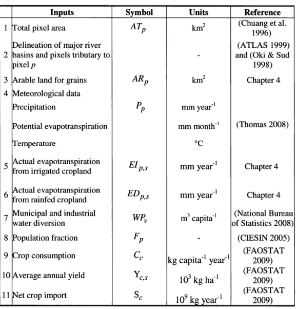
3.5 Sum m ary of Required Inputs... 54
4 Review of Available M odel Inputs... 57
4.1 Land-Related Inputs... 57
4.1.1 Study Area and M odel Grid...57
4.1.2 Delineation of Basin Boundary and Definition of Tributary Areas...59
4.1.3 Arable Land ... 61
4.1.3.1 Soil Properties ... 62
4.1.3.2 Slope ... 63
4.2 W ater-Related Inputs ... 71
4.2.1 Meteorological Inputs ... ... 71
4.2.2 Crop Sequence and Viability... 75
4.2.3 M unicipal and Industrial W ater Use ... 83
4.3 Production/Consum ption-Related Inputs... 85
5 Input Estim ation...89
5.1 Form ulation of the Input Estim ation Problem ... 89
5.2 Data Used for Estim ation of Unknown M odel Inputs ... 92
5.2.1 Total Population...92
5.2.2 Provincial Crop Production ... 93
5.2.3 Basin Runoff...96
5.2.4 Total Cropland ... 97
5.2.5 Total Irrigated Cropland... 99
5.2.6 Constraint-Related Inputs ... 102
5.3 Estim ates of Unknown Inputs ... 103
5.3.1 Estim ated Cropland...103
5.3.2 Estim ated Noncrop Evapotranspiration Rate ... 108
5.4 Estim ation Perform ance...109
5.4.1 Total Population...109
5.4.2 Provincial Crop Production ... 109
5.4.3 Basin Runoff...111
5.4.4 Total Cropland ... 112
5.4.5 Total Irrigated Cropland...114
6 Scenario Analysis under Nom inal and Changed Clim ates ... 115
6.1 Baseline Solution...116
6.2 Scenario Analysis with South-to-North Water Diversion and Climate Change ... 121
6.2.1 South-to-North W ater Diversion ... 121
6.2.2 Clim ate Alternatives from GCM s...127
6.2.3 Downscaling GCM Predictions ... 137
6.2.4 M odel Solutions for Clim ate Alternatives...147
7 Conclusions... 157
7.1 Summ ary of Results...157
7.2 Original Contributions ... 159
7.3 Future Research...161
Appendix ... 163
List of Figures
Figure 1-1: Trends in global water use by sector. ... 17 Figure 1-2: Trend in Chinese population. Black circles represent reported population from
1985-2008 by the National Bureau of Statistics of China. Blue triangles represent the predicted
mid-year population from 2009-2050 by the U.S. Bureau of Statistics...20 Figure 1-3: Trends in Chinese per capita consumption from 1990-2005 reported by The Food and A gricultural Organization... 20 Figure 1-4 (a)-(c): Annual average precipitation, potential evapotranspiration, and water
av ailab ility ... ... 2 3
Figure 1-5: Map of cropland distribution in China as a percentage of total area in each 0.5' pixel. It was constructed by combining census data from 1990 with Landsat TM from the years
19 9 5/19 9 6 ... ... 24
Figure 1-6: Population distribution over China in 2005. The legend shows number of people in each 0 .5 ' p ixel. ...- .--- ....--- .2 5 Figure 1-7: O utline of the thesis ... 30
Figure 2-1: The division between north and south regions for the simplified analysis...34 Figure 2-2: Graphical representation of the simplified problem when the objective function is to m aximize people fed or a is equal to zero... 37 Figure 2-3: Graphical representation of the simplified problem when the objective function is to minimize the deviation from existing conditions or a is equal to one...38
Figure 3-1: Daily caloric consumption in Chinese diet and contribution from the model food categories during 1990-2005 ... 43
Figure 3-2: Flow routing schem e... 45
Figure 4-1: China mask and model grid in geographical coordinates. ... 58
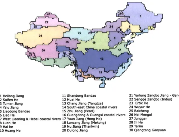
Figure 4-2: TRIP basin boundaries (red outline) overlaid on drainage basins map. They are shown with the original projection of the drainage basins map which is the azimuthal equal-area p rojectio n ... 6 0 Figure 4-3: River basins of the optimization model in geographical coordinates...61
Figure 4-4: Slope information over China from HYDROlk. ... 63
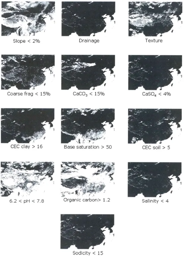
Figure 4-5: Maps of area where slope and soil characteristics are very suitable for maize (Class S I requirem ents)...67
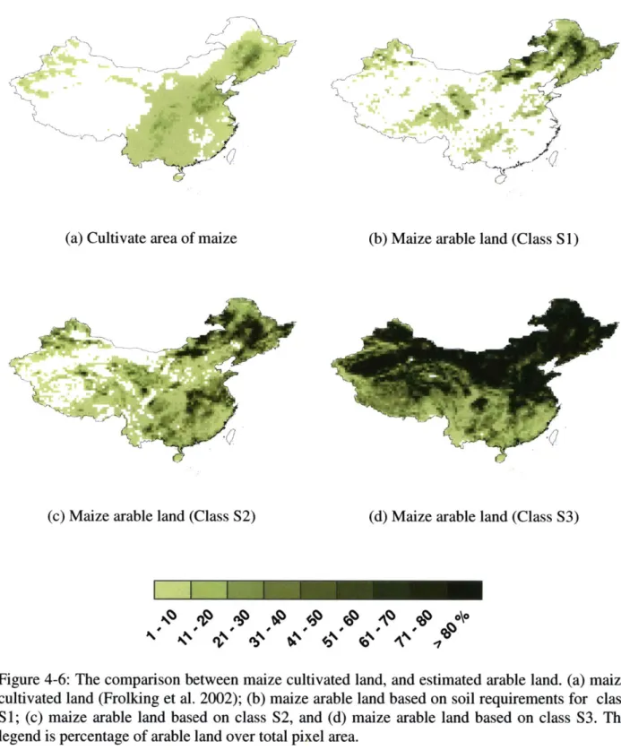
Figure 4-6: The comparison between maize cultivated land, and estimated arable land. (a) maize cultivated land (Frolking et al. 2002); (b) maize arable land based on soil requirements for class SI; (c) maize arable land based on class S2, and (d) maize arable land based on class S3. The legend is percentage of arable land over total pixel area. ... 68
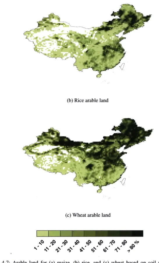
Figure 4-7: Arable land for (a) maize, (b) rice, and (c) wheat based on soil properties as a percentage of the total pixel area... 70
Figure 4-8: The average annual precipitation from 1951-1990...72
Figure 4-9: The average annual temperature from 1951-1990... 72
Figure 4-10: The average annual reference evapotranspiration. ... 75
Figure 4-11: A typical pixel showing a combination rainfed cropland, irrigated cropland, and noncrop area. ... 76
Figure 4-12: Time-dependent crop coefficient curve for the double cropping sequence fmr (fallow , m aize, rice). ... 80
Figure 4-13: The generalized single crop coefficient curve for perennial crops from (Allen et al. 19 9 8 ). ... 8 1 Figure 4-14: Provincial M&I water diversion per capita in 2007. ... 84
Figure 4-15: Population distribution over China in 2005 (CIESIN 2005). The legend shows num ber of people in each 0.50 pixel. ... 85
Figure 5-1: Average annual provincial crop production for the model's six crop categories during the period 1990-2000. The national amount is according to FAOSTAT and is scaled down to provincial level with data from China Statistical Yearbook (1997-2001)...95 Figure 5-2: Distribution of total cropland areas in China. The map shows the fraction of total land devoted to cropland in at least one season in each 0.50 pixel (Frolking et al. 2002). White indicates negligible cropland... 99 Figure 5-3: Map of fraction of irrigated area in 0.5' grid consistent with the cropland
distribution. W hite indicates negligible irrigated area...101 Figure 5-4: Provincial M&I water diversion per capita in 2004. ... 103 Figure 5-5: Model's estimated crop area devoted to (a) single-cropping; (b) double-cropping; (c) triple cropping. The map shows a fraction of crop area as a percentage of the total pixel area. 104 Figure 5-6: Model's estimated irrigated and rainfed crop area for (a) maize; (b) wheat; (c) rice. The left column is the irrigated area and the right column is the rainfed crop area. The map shows a fraction of crop area as a percentage of the total pixel area...106 Figure 5-7: Model's estimated irrigated and rainfed crop area for (a) oil crops; (b) tubers; (c)
vegetables. The left column is the irrigated area and the right column is the rainfed crop area. The map shows a fraction of crop area as a percentage of the total pixel area. ... 107 Figure 5-8: Estimated annual noncrop evapotranspiration rate...108 Figure 5-9: Comparison between model's estimate and observed provincial crop production. 110 Figure 5-10: Basin runoff comparison between the model's estimates and observations...111 Figure 5-11: Cropland distribution as a fraction of total area in 0.5grid from (a) observation; and (b) model's estimates. The third figure is the difference between model's estimates and observation in percent to the total pixel area...113 Figure 5-12: Irrigated area as a fraction of total area in 0.5grid from (a) observation; and (b) model's estimates. The third figure is the difference between model's estimates and observation in percent of the total pixel area. ... 114
Figure 6-1: Model's baseline people fed versus land use change in percentage...117 Figure 6-2: Increase in sown area, crop area, and irrigated area for three cases of land use change com pare to the nom inal condition...120
Figure 6-3: Increase in single-, double-, and triple cropping area for three cases of land use
change com pare to the nominal condition...120
Figure 6-4: The general layout of the South-to-North Water Diversion Project (Source: w w w .yellow river.gov.cn)... 122
Figure 6-5: The layout of ER P. ... 124
Figure 6-6: The layout of M R P. ... 125
Figure 6-7: The layout of W R P. ... 126
Figure 6-8: Number of models out of 24 GCMs that project increases in (a) winter precipitation and (b) summer precipitation over China for A IB scenario. Precipitation change between 1970-1989 and 2080-2099. ... 129
Figure 6-9: Precipitation change (%) from the years 1970-1989 to 2080-2099 for AlB scenario from 24 G C M s...13 1 Figure 6-10: Climatic regions in China. (Source: USDA Joint Agricultural Weather Facility). 133 Figure 6-11: Modified climatic regions to coincide with the river basins. Region I: steppe and desert; Region II: steppe; Region III: temperate continental; Region IV: subtropical wet, sum m er rain, and tropical w et and dry... 134
Figure 6-12 (a-d): The predicted changes in precipitation, temperature, and reference evapotranspiration in June from the years 1970-1989 to 2046-2065 under the AlB scenario from selected G C M s...145
Figure 6-13: Model's people fed versus land use change for the period 2045-2065 with the CGCM3.1 (T47) alternative (average over all models) compare with the baseline solution. ... 147
Figure 6-14: Model's people fed versus land use change for the period 2045-2065 with the
ECHAM5/MPI-OM alternative (Slightly drier in summer) compare with the baseline solution. 149 Figure 6-15: Model's people fed versus land use change for the period 2045-2065 with the
GFDL-CM2.1 alternative (Dry summer in Northwest and dry winter in Southeast) compare with
the baseline solution...15 1
Figure 6-16: Model's people fed versus land use change for the period 2045-2065 with the MIROC3.2.hires alternative (High summer rainfall everywhere) compare with the baseline so lu tio n ... 15 3
Figure 6-17: Model's predicted people fed versus land use change for the period 2045-2065 under climate alternatives compare with result from the baseline and the predicted peak population of 1462 m illion people...155
List of Tables
Table 1-1: Time periods used within this thesis. ... 30
Table 2-1: Inputs and solutions for two extreme values of a. ... 39
Table 3-1: The model crop categories and sub categories. ... 44
Table 3-2: Summary of the decision variables of the detailed model... 48
Table 3-3: Summary of available and derivable inputs for the detailed model...54
Table 3-4: Summary of unavailable inputs. ... 55
Table 4- 1: Physical and chemical properties provided in HWSD... 62
Table 4-2: Soil requirements for maize from Sys et al. (1993). ... 65
Table 4-3: Crop base temperature above which growth is possible. ... 77
Table 4-4: Crop Growing Degree Days requirement... 78
Table 4-5: Crop evapotranspiration adjustment coefficients for the seven model crop categories. ... 8 2 Table 4-6: Fractional time spent in each growth stage for each model crop category. ... 83
Table 4-7: Consumption and net import for each crop category in 2005. ... 86
Table 4-8: Yield values for each crop category for baseline simulation and climate change altern atives...87
Table 5-1: The national annual crop production data from FAOSTAT and China Statistical Yearbook averaged during the period 1997-2001 for the model's seven crop categories (spring and w inter w heat are com bined)... 93 Table 5-2: Mean annual runoff for all of the model's river basins (1956-1979)...96 Table 5-3: Average consumption rates, yield and net import during the calibration period for the model's seven crop categories (spring and winter wheat combined). ... 102
Table 6-1: Comparison of people fed and agricultural area between nominal condition and three levels of land use change...119 Table 6-2: Precipitation changes (%) between 2080-2099 and 1970-1989. Numbers in red
indicate decreases in change. GCMs highlighted with yellow color are selected alternatives. .. 135 Table 6-3: Selected climate alternatives from GCMs with precipitation changes (%) for two time periods compare to 1970-1989. Numbers in red indicate decrease in change. ... 136 Table 6-4: People fed and agricultural areas from three levels of land use change from the
C G C M 3. 1 (T47) alternative. ... 148
Table 6-5: People fed and agricultural areas from three levels of land use change from the
ECH A M 5/M PI-O M alternative. ... 150 Table 6-6: People fed and agricultural areas from three levels of land use change from the
G FD L -C M 2.1 alternative. ... 151
Table 6-7: People fed and agricultural areas from three levels of land use change from the
M IR O C 3.2.hires alternative. ... 153 Table 6-8: Agricultural land use from all alternatives to feed predicted peak population of 1462 million people and nominal land use from the period 1990-2000...155
Chapter 1
Introduction
1.1
Context
Increasing global population requires increasing demand for food. This entails increasing demand for the two basic natural resources needed for food production, freshwater and cropland. In 2000, agriculture already accounted for 67% of the world's total freshwater withdrawal
(UNESCO 2000).
190 1i59 1950 1975 20 200 1000 1M2 1960 17 Z 20M 100 1 195 101975 2000 20M8
*
do". m ef--- 0----S0.- W ---- m
0----oe eban.n, = he dferm betw.o .s ft amunt of waer extracted and Ot aifota *or"wosd Wftrnoy extracted, ud. voycd~ (o eurned to cove. or eowfrt* and ined koermed ate noa ZIO gtau octoohwmit lu. woomo Itwa~f *sco0d We Dbatbbduoeapcrdb
cukew pleer Fyil odik~itKatPo,k ftad wa Ubed HftEadmodoacote
Figure 1-1: Trends in global water use by sector. ... .. .... .. .. ......
The supply of arable land is largely limited by available water, soil conditions, and topography. Irrigation plays a significant role in bridging the gap between naturally available water and crop water demand, making it possible to increase crop production and expand cultivated land. About
10% of the earth's land surface is devoted to cropland, and 16% of this land is supplied with
irrigated water (Postel 1993). However, since the late 1970s, the rate of global irrigation development has dropped considerably due to soil salinization, the high cost of irrigation networks, the depletion of irrigation water sources, and other environmental problems. Thus, there is no easy solution for meeting the increasing food demand.
China is one of the countries that face the challenge of managing water and land resources to support their growing population. With a population of 1.32 billion in 2007 (National Bureau of Statistics 2008), China is the world's most heavily populated nation. Limitations on China's water and land resources are evident. China's total water resource in 2007 has been estimated to be 2,526x109 M3, with 2,424x 109 m3 of surface water and 762x 109 m3 of groundwater, and the
annual per capita water resource is low, at the level of 1,916 m3 per person in 2000 (National
Bureau of Statistics 2008). By comparison, the World Business Council for Sustainable Development considers that a country experiences water stress when the annual per capita water resource is less than 1700 m3 per person.
Furthermore, increasing trends in population and per capita consumption are observed. Figure 1-2 shows an increasing trend in Chinese population from 1985-1-2008 reported by National Bureau of Statistics (2008) (shown with black circles) while the blue triangles represent predicted
mid-year population from 2009-2050 by the U.S. Census Bureau. The United Nations estimates that China's population will reach its peak at 1.46 billion people by 2030. Changes in per capita consumption in the Chinese diet are also straining resources. Figure 1-3 shows trends in Chinese per capita consumption from 1990-2005 for four major crop categories: wheat, rice, maize, oil crops, and tubers (FAOSTAT 2009). The consumption here refers to a total domestic utilization quantity, which is the sum of the amount of feed, seed, waste, processing, food, and other utility. We see increasing trends in maize, oil crops, and tubers per capita consumption with an exception of slightly decreasing trends in rice and wheat consumption rates. The Food and Agricultural Organization reports per capita consumption (including food and feed) for maize has risen by almost 45% from 1980s to 2003. This increase in a large part due to the increase in meat consumption (feed part). Feeding 160 million more people with increasing per capita consumption is a challenge that some researchers feel cannot be met with available natural resources. For example, Brown (1995) believes that China is already operating beyond a sustainable level of production, a situation that they will have to import from other nation's to make up the difference between domestic production and demand.
Population 1500 1400 1300 1200 1100 1000 1990 2000 2010 2020 2030 2040 2050 Year
Figure 1-2: Trend in Chinese population. Black circles represent reported population from
1985-2008 by the National Bureau of Statistics of China. Blue triangles represent the predicted
mid-year population from 2009-2050 by the U.S. Bureau of Statistics.
Consumption Per Capita
0+-1990 1992 1994 1996 1998 2000 2002 2004
Year
Figure 1-3: Trends in Chinese Agricultural Organization.
per capita consumption from 1990-2005 reported by The Food and --- _- -______
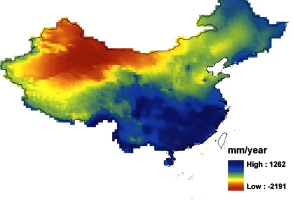
China's agriculture is further complicated by an uneven distribution of land and water resources. One of the main challenges of managing natural resources in China is that there is a mismatch between the location of water resources and available land. Water availability can be approximately quantified by the difference between precipitation and potential
evapotranspiration, as shown in Figure 1-4 (a)-(c) (Thomas 2007 and 2008). Precipitation is the original source of water supply in both surface and groundwater flows. Potential evapotranspiration is an upper bound of actual evapotranspiration (water demand) by crops. If potential evapotranspiration is high, there is a high demand in atmospheric moisture. As shown in Figure 1-4 (c), most of the country's available water is concentrated in the south, which experiences a strong monsoon climate.
nlyear
High: 2408
Low: I
(a) Annual precipitation average over the period 1951-1990.
1r
High: 2280
Low : 342
mm/year
High : 1262Low: -2191
(c) Water availability index (precipitation - potential evapotranspiration). The blue region is where precipitation is greater than potential evapotranspiration; while the red region is where potential evapotranspiration is greater.
Figure 1-4 (a)-(c): Annual average precipitation, potential evapotranspiration, and water availability.
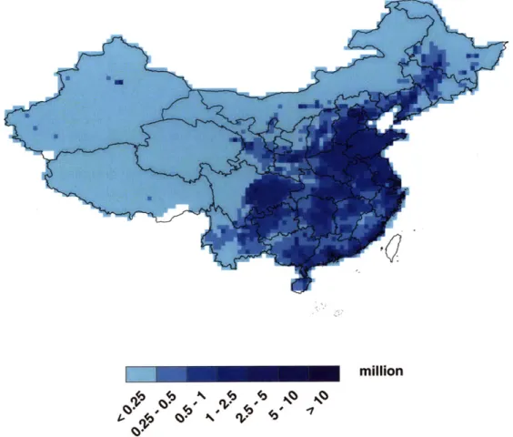
While water resources are most abundant in southern areas, cropland and population are concentrated more in the central and northern regions, where water is more limited. Figure 1-5 shows the extent of cropland distribution around 1995-1996 (Frolking et al. 2002) and Figure 1-6 below shows the population distribution in 2005 (CIESIN 2005). The population distribution more or less coincides with the cropland distribution and both differ noticeably from the water availability distribution in Figure 1-4 (c).
While there is large uncertainty in cropland estimates, many studies suggest that the land devoted to agriculture in China was on the order of 130 Mha in the late 1990's (Smil 1999). Smil (1995) reports that approximately 0.5 Mha of cropland have been lost every year since the early 1980's. As of the end of 2007, the cultivated area was reported to have dropped to 121.7 Mha (National Bureau of Statistics 2008). Factors contributing to the loss of arable land in China include conversion to other uses, desertification and afforestation. World Bank (2001) estimated that 331 Mha of land in China are prone to desertification. The area of cropland that was converted to forest in 2007 was estimated to be on the order of 85,000 ha (National Bureau of Statistics 2008).
**
Figure 1-5: Map of cropland distribution in China as a percentage of total area in each 0.50 pixel. It was constructed by combining census data from 1990 with Landsat TM from the years
million
Figure 1-6: Population distribution over China in 2005. The legend shows number of people in
each 0.50 pixel.
One of the extreme examples of the inconsistency in resource distributions is the North China Plain (NCP, areas around the lower reaches of the Yellow, Huaihe and Haihe rivers). This region accounts for one third of the national GDP, produces about half of the nation's wheat and one third of its maize, but only receives 7.7% of national water resources (Ministry of Water Resources, PRC 2004). Furthermore, 83% of China's irrigated land occurs in this semi-arid region, and it is estimated that the water tables in the three major river basins of the North China Plain (NCP) have dropped 50 m in some areas (World Bank 2001). A large scale project to divert water from the Yangtze River to alleviate water shortages in the NCP was initiated in 1950s. ... ... ... ... ... ... .. . .. .. ...
This South-to-North Water Diversion project is underway, with the construction of three major routes, and expected to divert 44.8 billion m3 year-1 by 2050, which is equal to the amount of
annual runoff of the Yellow River, to over ten provinces in the NCP, arid northwestern and northern regions.
An assessment of China's food production must account for future changes in the distribution of its natural resources. The South-to-North Water Diversion is designed to increase water availability in the northern part of the country. However, the effects of this project could be modified or even overwhelmed by climate changes that are very difficult to predict. Most global climate models (IPCC 2007) predict a warming trend over all China, but changes in precipitation subject to significant uncertainty. A combination of warming temperatures and changes in precipitation may have a significant impact on crop viability in different regions.
1.2
Literature Review
Will China be able to support its population with finite water and land resources? Smil (1995) provided an overview of China's food production capacity by investigating three critical issues. First, there were great uncertainties in the official estimates in the total area of China's cultivated land before the 1990's. The cropland was substantially larger than the official reports and as a consequence the estimated average yields were considerably too high, leaving room for improvement. Second, the use of national averages and generalizations misrepresented the complex realities of the country. Finally, there were opportunities for higher efficiencies in irrigation water and agricultural practice. Smil (1995) concluded that China should be able to continue support itself without drastic adjustments or substantially advance technology.
Another study conducted by IIASA (International Institute for Applied Systems Analysis) addressed this question using a detailed Agro-Ecological Zoning (AEZ) methodology (Heilig et al. 2000). The AEZ methodology uses a land resources inventory to assess feasible agricultural land-use options and to quantify the expected production of relevant cropping activities. They looked closely at changes in arable land, potentials for multi-cropping, urbanization and changes in diet. However, the assessment of China's arable land potential was only based on grain suitability under rainfed condition.
A more recent study investigated the effects of climate change on China's food production.
(Thomas 2006) simulated the potential yield for rainfed cropping systems during the period
1951-1990 and the climate scenarios for the year 2030 with gridded (0.250 X 0.25-) climate
dataset and digital soil data. The results showed that potential crop yields displayed a tremendous variation both in temporal and spatial respects during the period 1951-1990. Results for future scenarios indicated an enlargement of the subtropical cropping zone.
However, the studies by Heilig et al. (2000) and Thomas (2006) essentially ignored water demand from noncrop areas and non-agricultural water use. They also did not incorporate important information on networks of water movement and river basins in water balance calculation. Further, they did not include validation with observed conditions. They also did not include the South-to-North Water Diversion in their studies.
1.3
Research Questions
The aim of this thesis is to address the following questions:
1) What is the maximum food production possible with specified (existing or future) land
and water resources in China?
2) What are the effects of climate change and the South to North Water Diversion project on China's food production?
1.4
Research Approach
This thesis presents a systematic evaluation of how land and water resource limitations will affect agricultural production in China. Our approach is based on the following principles:
1) The focus of our study is to better understand how natural resources of land and water
limit crop production. As a result, we do not take into account the various economic factors that affect food production, such as policy, institutions, capital, and labor in our analysis.
2) Our approach is based on basic principles of: * Water balance
" Land balance
e Crop resource requirements
* Consumption requirements
Base on these four basic principles, the assessment of natural resources limitations on food production can be formulated into an optimization model, with the objective function maximizing the number of people fed subject to resource constraints. We begin our evaluation of water and land limitations on food production with a simplified model
and illustrate with it how water and land resources constrain food production differently in different regions in China.
3) We rigorously assess China's food production potential by formulating an optimization
problem (a detailed model) that includes a physically-based model that represents heterogeneous conditions and is calibrated with observations. Heterogeneities across meteorological, geographical, and dietary conditions are all considered. Specifically, we formulate the problem at the spatial and temporal resolutions needed to properly describe trends in climate, land use and crop parameters. This allows for fine scale networks of water movement in the model, along with water balance at the river basin scale. Complexity in diet is expressed using mixtures of crops. We assume that food can be freely transferred within the country.
4) The detailed model developed is calibrated to reproduce long-term observed conditions during the nominal or calibration period of 1990-2000 and used to estimate unknown model inputs.
5) We then use the model together with globally and locally available data and estimated inputs to simulate China's food production capacity during the year 2010 (Baseline simulation) and the future period of 2046-2065. Our baseline simulation relies on meteorological data from the period 1951-1990. The future predictions include the impacts of the South-to-North Water Diversion project and projected climate change. The future climate alternatives are selected from the general circulation models' prediction to represent diverse seasonal and regional patterns. A summary of the time periods used within this thesis is provided in Table 1-1.
Table 1-1: Time periods used within this thesis.
Time period Nominal/Calibration period 1990-2000
Baseline 2010
Climate change alternatives 2046-2065
Meteorological period 1951-1990
1.5
Thesis Organization
The content of the thesis is described below and outlined in Figure 1-7.
Chapter 2 Simplified Model Chapter 4 Available Model Inputs Chapter 3 Chapter 5
Detailed Model Input Estimation
Figure 1-7: Outline of the thesis.
We begin our evaluation of water and land limitations on food production with a simplified analysis in Chapter 2. In Chapter 3, we show how the simplified model can be extended to include heterogeneous representation of China's resources and hydrologic flux balance. The full
Chapter 6
Scenario Analysis under Nominal and Changed Climates
formulation of the detailed optimization problem is presented in this Chapter. Chapter 4 is devoted to a comprehensive review of available inputs for the model. Then we discuss how to estimate some inputs that are not readily available and derivable from other data in Chapter 5. In Chapter 6, we present a scenario analysis of China's food production during the future period of
2046-2065 under nominal and changed climate using the model of Chapter 3, and data and inputs
discussed in Chapter 4 and 5. Chapter 7 summarizes results from this research and original contributions, and discusses suggestions for future improvements of the model.
Chapter 2
Simplified Model
This main objective of this research is to evaluate the land and water resources limitations on food production. In this chapter, we introduce a simplified analysis based on the basic principle of land balance, water balance, and food consumption and production balance. We present the formulation of the simplified problem and illustrate with it how water and land resources constrain food production differently in different regions in China.
2.1
Simplified Problem Formulation
In China, both water and cropland resources are unevenly distributed across the country. While the southern region receives much more rainfall, arable land is more concentrated in the eastern
and northern regions. For the simplified analysis, we assume that:
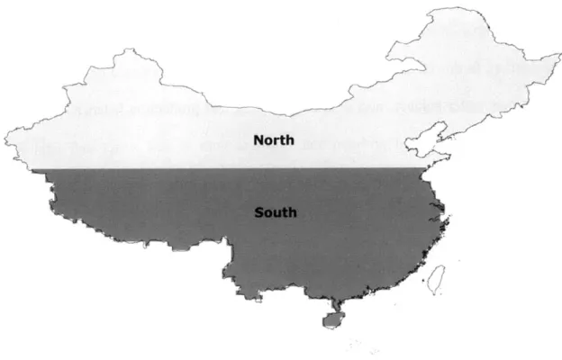
1) China is divided into two regions, north and south as shown in Figure 2-1.
2) Land is categorized as cropland or noncropland. Noncropland includes both natural and built environment that are not used for agriculture.
3) For crop type, we simply consider the aggregation of major grains that are grown in
China, which are maize, rice, and wheat.
4) Cropland is further constrained by the total arable land. Arable land here refers to land with adequate accumulated degree days in a year, suitable soil characteristics, and slope for those three grains.
5) Precipitation is the only source of available water. This implies that water can be stored intra-annually and can be readily transported anywhere in each region.
North
Figure 2-1: The division between north and south regions for the simplified analysis.
To determine how many people can be fed subject to water or land limitation in each region, we formulate a multi-objective optimization to maximize the number of people fed and minimize an adjustable mean-squared deviation of cropland from nominal values subject to land and water
resource constraints. The primary unknown in this simplified problem is the amount of cropland for each region. The inputs and results are annual long-term averages.
The problem can be formulated as shown in Equations (2-1) to (2-5) below. In the objective function, the first term is a maximization of number of people fed and the second term is a minimization of the deviation of cropland from nominal values, as shown in Equation (2-1). a is an adjustable weighting factor indicating priority given to the second term. For a equal to zero, priority is given entirely to maximizing the number of people fed. When a is increased, more weight is placed on the land deviation term. Equations (2-2) to (2-4) represent land and water constraints for each region. Cropland is converted into number of people fed via yield and consumption rates in Equation (2-5).
Objective function:
Maximize peoplefed -a I
||croplandi
-nominal cropland;||2 (2-1)i=N,S
Decision variables: peoplefed, croplandi
Land constraints (i = N, S):
cropland; +noncropland; = totallandi, (2-2)
cropland; arablelandi, (2-3)
Water constraints (i = N, S):
Production-Consumption balance:
(peoplefed )( consumption )= X (cropland; )( cropyield) (2-5)
i=N,S
2.2
Problem Solving and Solutions
This simplified model is a quadratic programming problem (QPP) since it has a quadratic objective function and only linear constraints. Using a quadratic programming formulation allows for a computationally efficient solution of the problem. Moreover, with all linear constraints, the feasible region of the optimization problem is convex, while its objective function is strictly concave. With these two conditions, a unique solution is guaranteed for the detailed model (Bradley et al. 1977).
We can solve this simplified problem manually for two extreme values of a using graphical method. When a is equal to zero, the objective function becomes a maximization of people fed. The objective function can be rewritten using the relationship in Equation (2-5) between the number of people and the unknown cropland in north and south regions. Figure 2-2 shows a graphical representation of the feasible region with the linear objective function. The inputs for the simplified problem are summarized in Table 2-1. The arable land constraints (green lines) are from Equation (2-3). Equation (2-4) together with Equation (2-2) form water constraints (blue lines). The red dash lines are the objective function with different levels of people fed. The red arrow indicates a direction of increasing number of people fed. The optimal cropland in this case is thus the intersection between the water constraint of the northern region and the arable land constraint of the southern region.
Cropland (north) 10' ha 210 57 Objective function Cropland (south) 106 ha
Figure 2-2: Graphical representation of the simplified problem when the objective function is to maximize people fed or a is equal to zero.
For the case of a equal to one, the constraints remain the same but the objective function depends only on the deviation from existing conditions. Here, the objective function is a circle with a center at the existing conditions. Figure 2-3 shows a graphical representation of this case with the red arrow indicating the direction of decreasing value of the deviation term. The optimal cropland allocation in this case is equal to the values of existing conditions.
Cropland (north) 106 ha Arable land constraints 210 Objective function Water constraints 57-Feasible region -Optimal soluti (65,33) Cropland (south) 106 ha 87 944
Figure 2-3: Graphical representation of the simplified problem when the objective function is to minimize the deviation from existing conditions or a is equal to one.
When a is between zero and one, there is a tradeoff between the number of people fed and the deviation from nominal conditions. Table 2-1 summarizes inputs and results for the two cases. The uneven resources distribution in China is clear from the precipitation and arable land data. The mean annual precipitation in the south is more than three times higher than in the north while arable land in the north is much more abundant than in the south. Other inputs, except for evapotranspiration from noncropland are assumed to be uniform and the same for both regions.
Table 2-1: Inputs and solutions for two extreme values of
North
Total land' 459
Grains arable land2 210
Observed grains cropland3 33
Precipitation4 280
Grains water demand5 700
Grains consumption6 330
Grains yield7 4880
Non arable land ET8 220
a. South 491 87 65 940 700 330 4880 440 Matching observation Cropland 33 65 Flow to ocean 117 2286
Total people fed 1.4 109 Maximizing peoplefed
Cropland 57 87
Flow to ocean 0 2229
Total people fed 2.1 10
Data sources: 1. (Chuang et al. 1996)); 2. Section 4.4; 3. (Frolking et al. 2 Section 4.3.2; 6. (FAOSTAT 2007a); 7. (FAOSTAT 2007b); 8. Chapter 5
Units 106 ha 106 ha 106
ha
mm/yr mm/yr kg/(capita-yr) kg/ha mm/yr 106 ha km3 106 ha km3 002)); 4. (Thomas 2007); 5.As mentioned above, the weighting factor, a, allows us to examine the problem in two different ways. When a is equal to one, priority is entirely given to matching existing conditions. The optimal result for this case matches the observed cropland for both regions exactly, and the number of people fed is 1.4 billion. This calculated number of people fed is close to the current population of 1.3 billion, which provides some confidence in the model. On the other hand, when a is equal to zero, the amount of cropland calculated in the optimization problem deviates notably from existing conditions, and the calculated number of people fed jumps to 2.1 billion. Cropland in the south reaches the extent of the total arable land for this solution. In the north, even though arable land is abundant, only one fourth is allocated as cropland because of limited
water resources. These results show significant potential for increasing food production in China, yet it is in ways that could involve dramatic changes in land use.
In conclusion, our simplified optimization model is able to provide a rough estimate of how many people China can feed, given a specified priority for matching existing land use conditions. Although the model as formulated above is highly simplified, results from it serve to highlight the importance of including a penalty term for deviations from existing conditions. Without this term, the model could predict a scenario that is very optimistic in terms of production capacity, but involve significant and unrealistic land use changes. Therefore, the penalty term implicitly serves as a simplified representation for other constraints not included in the model such as economic, institutional, and political conditions.
The simplified problem presented in this Chapter provides a basis for understanding where land or water resources limit food production in China. The northern region has abundant arable land with limited water resources. In contrast, in the south, arable land is the limiting factor. The simplified problem provides a good basis from which to build a more sophisticated model that can appropriately characterize China's resources distribution, as well as natural and managed conditions. In the following Chapter, the motivations for the improvements needed for the detailed model are outlined and the full formulation of the detailed model is presented.
Chapter 3
Detailed Model
In this Chapter, we begin by considering how the simplified model of Chapter 2 can be extended to include a more realistic heterogeneous representation of China's resources and hydrologic flux balance. Then we present the full formulation of the detailed optimization problem for evaluating food production capacity in China. The detailed version of the model provides a basis for predictions of the population that can be sustainably fed under various scenarios. Finally, we conclude with a summary of required data for the detailed model.
3.1
Motivation for A More Detailed Model
Although the simplified model of Chapter 2 predicts a number of people fed that is close to the current population when matching nominal conditions (a is equal to one), it ignores many realistic features such as spatial and temporal heterogeneity in climate, land use and crop parameters within each region, water balance at the river basin scale, and the mixture of crops in people's diet. This reduces its credibility for predicting the response to changes in climate, arable
land, and diet as well as the impact of large infrastructure project such as the South-to-North Water Diversion. In this section, we highlight the major limitations of the simplified model and outline the improvements needed to provide credible predictions of food production in China.
Spatial Variability
In the simplified problem of Section 2.1, we divided China into only two regions. However,
climate and land use over China are greatly heterogeneous. To account for the heterogeneity, China should be divided into much smaller units. Because much of the available data are
available at the resolution of 0.50 by 0.50, this is a convenient size to adopt for our analysis unit,
which we will refer to as a pixel. The size of a pixel is about 2,500 km2. There are about four
thousands pixels covering mainland China.
Crop Type
In the simplified model, only a single crop type was considered. However, all the main crop
types consumed in China should be included in the extended model in order to represent the typical Chinese diet. Figure 3-1 illustrates the average daily breakdown of the food types included in the Chinese diet, expressed in caloric content (FAOSTAT 2009). The largest food groups are wheat, rice, maize, starchy roots (tubers), oil crops, vegetables, meats, milk, and eggs which comprise at least 90% of the daily caloric demand in China for each year from 1990-2005. The daily caloric consumption per person increased about 300 calories during this period. There is a decreasing trend in cereals consumption and an increasing trend in oil crops, vegetables, meat, and eggs consumption.
Daily Food Consumption in China
3500 Z000-2500 - 2000- 1500-1000 500 1990 1992 1994 1996Figure 3-1: Daily caloric consumption categories during 1990-2005.
9% 91% 91% 91% 91% 90%
92%
92%
92%
92%
1998 2000 2002 2004 2006 Year
in Chinese diet and contribution from the model food
Domestic utilization provided in (FAOSTAT 2009) includes crop use for direct food consumption, animal feed and seed, and other net uses. The domestic crop utilization thus implicitly includes animal products consumed in the Chinese diet. In total, there are seven crop categories considered in the model. Among them, starchy roots (tubers), oil crops, and vegetables categories include several sub-species. Adding one more crop category from seven crops would result in 185 more possible crop sequences for each pixel (one more single, 15 more double, and 169 more triple sequences) .We represent these crop categories as a multiple-crop group in order to control the complexity of the model. Table 3-1 summarizes the seven model crop categories and their main sub species according to (FAOSTAT 2007b).
Wheat
-
Rice Maize-
Starchy roots Oil crops M Vegetables M Meat M Milk M Eggs-o- Total food consumption . ... ...
Table 3-1: The model crop categories and sub categories. Individual crops sub-category category Spring wheat Winter wheat Rice Maize
Tubers cassava, potatoes, sweet potatoes, yams
Oil crops soybeans, groundnuts, sunflower seed, cottonseed, coconuts, sesame seed, palm nuts-kernels, olives, linseed Crop group tomatoes, onions, garlic, carrots and turnips, cauliflowers
and broccoli, leeks, cabbages, lettuce, cucumbers, Vegetables pumpkins, squash, and gourds, green peas, green beans,
artichokes, asparagus, mushrooms, chillies, watermelons, other melons, eggplants, spinach
Imports and Exports
The simplified model considers China's domestic production. According to FAOSTAT, China imported more oil crops than the amount that was domestically produced in 2005. On the other hand, cereal imports were close to exports, which were about 3.5 percents of domestic cereal production (FAOSTAT 2007a). We need to account for the amount of imports and exports in the detailed model in order to insure flexibility for analysis of alternative scenarios.
River Basins and Flow Routing
In the simplified model, the water balance is greatly simplified with precipitation and evapotranspiration evenly distributed over each half of the country. It was also assumed that water can be readily transported anywhere in each region. However, precipitation and evapotranspiration vary greatly throughout the country and water can only be moved naturally via gravity or artificially through infrastructure. A more realistic model needs to incorporate an
accurate water balance that accounts for the movement of water. Since precipitation and evapotranspiration vary at scales much smaller than river basins, it is necessary to perform water balance calculations at both pixel and basin scales. Flow routing information is necessary for these calculations. The model needs to know the pixels tributary to each pixel as well as the identity of all pixels included in each river basin. Figure 3-2 shows an example of a drainage basin and its flow routing. The red arrow represents flow direction of each pixel. In this example, tributary or upstream pixels of pixel no. 6 are pixel no. 1 and 2. Pixel no. 12 is the outlet of the basin.
0.5 0
Figure 3-2: Flow routing scheme.
Typically, high resolution topographic data are used to determine flow directions and delineate the boundaries of a river basin. There are about thirty major river basins in China. We assume that these basins are self-contained, and there is no distinction between surface and groundwater
flows.
3.2
Decision Variables
Decision variables are the problem unknowns that are adjusted to maximize or minimize the objective function. This section describes the decision variables introduced by the model enhancement summarized in Section 3.1.
3.2.1 Crop Categories
The crops included in the model are winter wheat, spring wheat, rice, maize, tubers, oil crops, and vegetables. Winter wheat and spring wheat are assumed to have the same expected yield and are counted as one crop for consumption purposes. The model is intended to simulate crop production, but the Chinese diet also includes meats, milk, and eggs. These animal products are not included directly but are accounted for by the crops they consume. In this model, meat produced from grazing is neglected both in the diet and in production.
3.2.2 Crop Sequence
In China, roughly half of the cropland is cultivated for more than one season per year (i.e. is multicropped) (Frolking et al. 2002). We allow up to three crop sequences to grow in one calendar year in the model. Winter wheat is unique from the other sequences because it can only be grown over the winter. When there are no constraints 7 crops give 49 double-crop combinations and 343 triple-crop combinations. When the winter wheat constraint is added these figures drop to 42 double-crop and 252 triple-crop combinations. The total possible crop sequences from one-, double-, and triple-crop sequences are 301.
3.2.3 Irrigated vs Rainfed Agriculture
In the simplified model, we assumed that water supply from precipitation can be transported anywhere in each region. However, we need infrastructure to store rainfall that falls on
noncropland and off growing season, and a system to deliver this water supply to crop fields. Irrigation plays a major role in improving and expanding agricultural practices in China. Approximately 47% of China's cropland is irrigated (Doll & Siebert 1999). Therefore in the detailed model, we distinguish between cropland that is irrigated and rainfed. Crops can be grown on an irrigated pixel so long as water demand can be met throughout the growing season from water flowing from tributary (upstream) pixels. Crops that are not grown on a non-irrigated pixel must obtain enough water to sustain their growth from precipitation falling only in that pixel. This is known as rainfed agriculture.
The primary decision variables for this model are LIp's and LD, the amount of irrigated cropland devoted to crop sequence s in pixel p and the amount of rainfed cropland devoted to crop sequence s in pixel p, respectively. Several of the remaining decision variables, such as
basin runoffs Rb, evapotranspiration E, and Ep,nc and municipal and industrial water loss to evaporation Wb, appear in the water balance constraints. The production variable MAC , and the number of people fed N, appear in the food balance constraints. The list of the model's decision variables are summarized in Table 3-2 below.
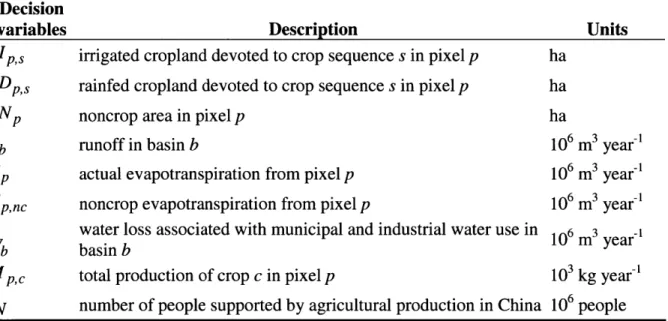
Table 3-2: Summary of the decision variables of the detailed model
Decision
variables Description Units
LIirrigated cropland devoted to crop sequence s in pixel p ha L s rainfed cropland devoted to crop sequence s in pixel p ha
LN, noncrop area in pixel p ha
Rb runoff in basin b 10 m year
EP actual evapotranspiration from pixel p 106 M year-Ep,nc noncrop evapotranspiration from pixel p 106 M
year-water loss associated with municipal and industrial year-water use in 106 M3 year-1
Wb basin b
MPc total production of crop c in pixel p 103 kg year-i
N number of people supported by agricultural production in China 106 people
3.3
Objective Function
The objective of the detailed model maximizes the number of people fed while minimizing the misfit between simulated and nominal conditions. However, now the nominal condition is described by the cropland in each pixel for each crop sequence during the calibration period:
minimize LIpsLD ps,N F(N,LIPS, LDP,S) 2 LD
Ps
- LDOP
s
P's LD0 IP N -a (3-1)Here LI0 p'sis the nominal or calibration period
calibration
irrigated cropland [ha], LD0 is
p's
period rainfed cropland [ha], while LI)
and LD>
the nominal or
are the corresponding
prioritized toward maximizing people fed or matching calibration period conditions, as discussed in Chapter 2.
3.4
Constraints
3.4.1 Land Constraints
Total area for pixel p:
In each pixel, a total land area is divided into cropland and noncropland. The total cropland is a summation of irrigated and rainfed cropland devoted to each crop sequence. Therefore, the total area is expressed as follow:
I ( Li p's + LDp's) + LNP = ATp, (3-2)
se all crop sequences
where AT, is the total land in pixel p [km2].
Arable land constraint for pixelp:
There are several factors that determine whether an area is suitable for growing crops. Temperature, crop water demand, slope and soil suitability are key factors. In our model, arable land strictly refers to an area that has suitable slope and soil properties for agriculture. Soil properties considered in the model include physical soil characteristics, soil fertility, and salinity and alkalinity. Section 4.4 explains in detail how we quantify arable land area from soil properties. The arable land constraint is only applied to maize, rice, and wheat. Due to the aggregation of the three food groups of tubers, oil crops, and vegetables, we could not apply the soil suitability approach to them since the soil requirements are different for each species in the
category. However, the amount of cropland for tubers, oil crops and vegetables is implicitly controlled by dietary demand.
There are three upper bound constraints on the total cropland, one for each crop, as shown in Equation (3-3).
Maize: (LIp,s + LDp,s )AR,maize,
se seq with maize
Rice: I ( Lip's + LDp,s) ARp,rice, (3-3)
se seq with rice
Wheat: I ( LI, ps + LDP, ) ARp,wheat> se seq with wheat
where ARp,crop is the total arable land in pixel p for the specified crop [km2]. Note that the summation of the cropland is not over all crop sequences. There are 115 crop sequences that include maize and 115 that include rice. The 146 crop sequences for wheat include both spring and winter wheat.
3.4.2 Water Constraints
Annual water balance for river basin b:
Our climatological analysis considers long-term average conditions. This can be equated with steady-state conditions for water balance, because the change in water storage within a unit area is negligible over time-scales greater than one year. Using this steady-state assumption, the basin water balance equation becomes
Pb - Eb -Wb = Rb, (3-4)
where Pb is the total basin precipitation [106 m3 year'], Eb is the non-municipal and industrial