HAL Id: hal-01511892
https://hal.archives-ouvertes.fr/hal-01511892
Submitted on 21 Apr 2017
HAL is a multi-disciplinary open access
archive for the deposit and dissemination of
sci-entific research documents, whether they are
pub-lished or not. The documents may come from
teaching and research institutions in France or
abroad, or from public or private research centers.
L’archive ouverte pluridisciplinaire HAL, est
destinée au dépôt et à la diffusion de documents
scientifiques de niveau recherche, publiés ou non,
émanant des établissements d’enseignement et de
recherche français ou étrangers, des laboratoires
publics ou privés.
Evolved Developmental Strategies of Artificial
Multicellular Organisms
Jean Disset, Sylvain Cussat-Blanc, Yves Duthen
To cite this version:
Jean Disset, Sylvain Cussat-Blanc, Yves Duthen. Evolved Developmental Strategies of Artificial
Multi-cellular Organisms. 15th International Symposium on the Synthesis and Simulation of Living Systems
(ALIFE XV 2016), Jul 2016, Cancun, Mexico. pp. 1-8. �hal-01511892�
O
pen
A
rchive
T
OULOUSE
A
rchive
O
uverte (
OATAO
)
OATAO is an open access repository that collects the work of Toulouse researchers and
makes it freely available over the web where possible.
This is an author-deposited version published in :
http://oatao.univ-toulouse.fr/
Eprints ID : 17069
The contribution was presented at ALIFE XV 2016 :
http://alife2016.alife.org/
To cite this version :
Disset, Jean and Cussat-Blanc, Sylvain and Duthen, Yves
Evolved Developmental Strategies of Artificial Multicellular Organisms. (2016)
In: 15th International Symposium on the Synthesis and Simulation of Living
Systems (ALIFE XV 2016), 4 July 2016 - 8 July 2016 (Cancun, Mexico).
Any correspondence concerning this service should be sent to the repository
administrator:
[email protected]
Evolved Developmental Strategies of Artificial Multicellular Organisms
Jean Disset
1, Sylvain Cussat-Blanc
1and Yves Duthen
11University Toulouse 1 Capitole - IRIT
{disset; cussat; duthen}@irit.fr
Abstract
We present the use of a new computationaly efficient 3D physics model for the simulation of cells in a virtual sea world. In this model, cells can freely assemble and discon-nect along the simulation without any separation between the developmental and evaluation stages, as is the case in most evo-devo models which only consider one cell cluster. While allowing for the discovery of interesting behaviors through the addition of new degrees of freedom, this 3D center-based physics engine and its associated virtual world also come with their drawbacks when applied to evolutionnary experiments: larger search space and numerous local optima. In this paper, we have designed an experiment in which cells must learn to survive by keeping their genome alive as long as possible in a demanding world. No morphology or strategy is explicitly enforced; the only objective the cells have to optimize is the survival time of the organism. We show that a novelty metric, adapted to our evo-devo matter, improves the outcome of the evolutionary runs. This paper also details some of the devel-opmental strategies the evolved multicellular organisms have found in order to survive.
Introduction
Over the past two decades, the artificial life community has seen the development of several models for the simulation of the environment in which cells can freely evolve. Many 2-dimensional models have been used, mainly for their sim-plicity and their computational efficiency, (Doursat, 2009; Joachimczak et al., 2013), but also because they are often sufficient to let interesting cellular behaviors emerge. With the addition of the third dimension comes both large possi-bilities in the exploration of artificial life as well as the excit-ing opportunity to more precisely compare and understand real world observations. While there are several 3D physics engines and simulators developed specifically for artificial life (Joachimczak and Wr´obel, 2011; Fontana and Wr´obel, 2013; Doursat and S´anchez, 2014; Cheney et al., 2014) com-bining low scale features of cells with efficient simulation at the scale of a whole organism can prove challenging, and always requires either ignoring interesting aspects of cells, such as their polarisation system, complex adhesive proper-ties, and variable stiffnesses, or abandoning computational efficiency.
Of course, many models of cellular simulations are not di-rectly linked to the alife comunity (although some have been used for artificial life experiments) and are more tightly re-lated to bio-simulation and focus on having engines that be-have in a bio-realistic manner. Over the years, many mod-els have been developed using various approaches, among which 2D lattice based cellular automata (Ouchi et al., 2003), various off-lattice 3D center-based models and even precise hybrid multi-scale systems which combine cell-level deformations as well as tissue-scale constraints (Lowengrub et al., 2009), to cite just a few. In the context of artificial life, and specifically when growing multicellular artificial organ-isms, the complexity of the simulated world directly im-pacts the developmental strategies and possible morpholo-gies of the creatures. As this can make for some behav-iors and strategies that are more desirable and might also help in the understanding of real-life behaviors by bring-ing more realism, it also comes with at least two obvious trade-offs. First, adding realism and complexity to the arti-ficial world will increase the required computational power, which is a resource of prime importance when using genetic algorithms that require the simulation of thousands of in-stances of these worlds. Secondly, and still in the context of artificial evolution, adding complexity to the world can dramatically broaden the search space, requiring even more simulations for evolutionary algorithms to come up with a convincing organism, and potentially complexifying the fit-ness landscape. It can thus be argued that the simulation of cells for the growth of artificial multicellular organisms is, while sharing obvious common roots, a different problem than the simulation of real world cells. Thus, while we take our inspiration from biology when designing a cell simula-tion engine, it is of prime importance to keep these trade offs in mind and to try and see where the truly desirable features lie, those from which an evolved multicellular or-ganisms might benefit, and those that can be simplified.
In this work, we propose to step up artificial life exper-iments in the third dimension using a fast cellular physics engine tailored to artificial life, MecaCell, that offers novel cell-cell interaction such as collision, adhesion and
vol-ume conservation approximation while keeping the com-putational cost in reasonable limits. We have designed an experiment in which the virtual multicellular organism will have to face many local optima created both by the added degrees of freedom and the rules of the world in which it evolves. We show how novelty search with a morphology metrics can, when used in conjunction with a fitness func-tion, help overcome many of these local optima. The ex-periment we present in this paper challenges one cell to pre-serve its genetic material in a sea-like environment as long as possible. In order to do so, the cell (which can choose to eventually become an organism after division) will have to face harsh conditions where energy is a difficult resource to harvest. Organisms, or rather same-DNA cell colonies, will thus have to balance their in-water morphology to collect light energy while maintaining solid roots in the ground in order to collect a second essential type of energy. While di-vision of labor might play a determining role in the survival of the colony (harvesting nutrients and light, sharing energy, maintaining the structure of the organism), the rules of the simulated world should make for the appearance of differ-ent viable strategies. In the lineage of our previous work (Disset et al., 2014), and to reduce the clues provided by a heavily engineered fitness function as much as possible, the cell controllers, based on gene regulation, are only evolved for survival (duration of the simulation) in addition to the novelty search criterion studied in this paper.
Simulated world
This section presents the different aspects of the simulated world we propose to investigate1. The main goal is to
try various characteristics of the physics engine, to explore ways to mitigate the adverse effect of adding degrees of free-dom (comparatively to a 2D simulator or a 3D cell simula-tor which doesn’t account for precise dynamic adhesions, for example). We want our virtual organisms to be able to evolve efficient and various solutions to the problem of sur-vival in a constrained environment.
Cell physics - MecaCell
MecaCell2 aims to be an artificial life friendly and generic
platform for the 3D simulation of cells. Its goal is to provide a continuous physics environment that is computationally efficient and versatile enough to tackle various aLife exper-iments and configurations (with exotic or simplified physics rules, for example).
1
All the source code as well as images and videos are available at https://github.com/jdisset/seacells
2MecaCell is written in C++ and available (under LGPL
li-cense) at https://github.com/jdisset/MecaCell. It includes a custom OpenGL display engine with a plugin system for the extensibility of its interface.
Cell and volume conservation In MecaCell, each cell is an agent represented by a center, a membrane and an orien-tation. A cell can freely evolve in a 3D continuous environ-ment, where it will collide and adhere with other cells. Here we consider cells to be spherical objects filled with a mostly incompressible fluid and wrapped in an elastic membrane. Every cell has a rest radiusRr and a dynamic radiusRd.
The dynamic radius was introduced to allow for the approx-imation of volume conservation: each time stept, if a cell is cut (overlapping either another cell or a 3D object), we re-compute both its membrane surface areaAtand its current
volumeVt. The net difference in volume relative to its rest
valueVris then translated into a stress pressurept:
pt= I × (V t− Vr)
At
whereI is the compressibility coefficient of the cell. Cell pressure acts as a force governing the growth of the dynamic radius. In an intuitive manner, when pressure increases un-der mechanical stress, the cell will compensate by expand-ing its radius in order to recover its original volume. But this variation also implies a modification of its current membrane surface areaAt, which will also act as a shrinking force on
the dynamic radius. The cell membrane is thus, in a com-putationally efficient manner, brought into equilibrium be-tween volume conservation and surface area conservation, using the following explicit integration scheme:
Rdt= Rdt−1+ ∆2× (∆V − ∆A −dRd dt × C)
where∆V is the volume variation Vt−Vr,∆A is the surface
area variationAt− ArandC is a damping coefficient.
Collisions In this model, collisions are easily handled by detecting two overlapping cells and by computing the nor-mal and the area of the resulting contact plane. Each cell will then push on the other perpendicularly to this plane and according to their internal pressure (resulting from their de-formation). The intensity of the force applied between a cell Caof internal pressurepaand a cellCb(with internal
pres-surepb) through a contact plane of areaAcis given by:
|| !F || = Ac× (Pa+ Pb)
withPi=!0,
ifpi< 0
pi, otherwise
A tunable damping termCcolis also added.
Adhesions When wanting to simulate artificial multicellu-lar organism in a 3D environment, the capability to maintain oriented connections is of prime importance. In MecaCell, cell-cell adhesions use the same kind of contact planes than for the collisions. A cell can choose its adhesive properties distribution across its membrane through the definition of an
adhesion functionfadhwhich associates an adhesive
recep-tor densitydadhto a unit vector expressed in the local
coor-dinate system of the cell (and represents the adhesive poten-tial at a given membrane location). We simulate an adhesion between two cells by the creation of a dynamic mass-spring-damper system of length 0, attached to the centers of the contact surfaces on both cells membranes. This spring acts on both membranes but all of the generated forces and mo-mentum is applied at the respective cells centers. When the two adhesive cells get closer from each other, the centers of the adhesion planes are updated, as well as all the mechan-ical properties of the adhesion mass-spring-damper system. The stiffnessK and damping coefficient C are proportional to the contact plane surface area as well as the average recep-tor density on said surface (and to the intrinsic characteris-tics of these receptor, which can be different for every cells, or favor certain cell-cell affinities between particular cellular types). When two adhesive cells are pulled apart (or rotated in different directions), the adhesive dynamic mass-spring-damper system can elongate up to a certain length defined by the maximum lengthMlreachable by an adhesion receptor.
Thus, if the cells are pulled apart too strongly (relatively to the strength of their connection), they can actually come out of contact again. Similarly, if they experience a torque of too much intensity or a shear stress above a certain thresh-old, they will be able to slide on each other’s membrane (as the centers of their adhesion plane will have moved too far apart due to rotation).
Environment - Ground and sea
In this experiment, the world is divided in two parts: the ground and the sea.
Ground The ground is a dense medium in which cells can-not easily move. In order to achieve this effect, we used a special integrator which does not take into account any iner-tia term, using only the force exerted on each cell to compute its next position. This ground acts as a solid when the forces exerted by the cells are below a certain threshold, only lowing cells to move if they push hard enough. This is, al-though in a simplified manner, a depiction of the mechanical characteristics of dense mud.
The ground contains nutrients, which are not available in the water. They are present in the mud at various depth, in small areas and finite amounts. At the beginning of the sim-ulation, we initializeN = 200 nutrients sources. For a given nutrient sourcei placed at a random position (xi, yi, zi) in
the mud, the initial amount of nutrientniis given by:
ni= Qn∗ (1 + Cn× |yi|Pn
)
whereQnis a constant andPnandCn are two parameters
that determine how the amount of nutrient varies for each nutrient source according to its depthyi. This is meant to
mimic how the nutrient distribution can be different accord-ing to the type of soil. It also allows for the tunaccord-ing of some aspect of the fitness landscape: withCn < 0, the selective
pressure would force the cells to expand laterally while a positive value ofCn should favor a vertical growth to find
more reliable sources of nutrients. In this particular expe-rience, we useQn = 0.03, Pn = 1.5 and Cn = 0.035.
These values have been chosen empirically in order to make a environment in which organisms can survive easily for a short amount of time but must develop complex strategies to survive longer.
Sea The second layer of the world is placed on top of the first ”mud” layer. We call it water, because its mechanical characteristics, namely density and viscosity, are supposed to mimic those of a still body of water. Here, a classic semi-implicit Euler integration scheme is used to update the cell positions and orientations. For the sake of computational duction, no flows are simulated in this water. This would re-quire hydrodynamics to be simulated, which would be very expensive to compute. However, the cells are all slightly buoyant which means that they need to keep adhesions to cells that are still inside the mud in order to avoid being taken away.
Light is abundantly available in the water but stopped by the ground. It only comes in straight rays, perpendicular to the ground, and if one light ray shines upon a given cell, it won’t be able to reach any other cell below that first one. In other words, cells block light and their shadows prevent other cells to be lit. We implemented this feature using a classical depth-buffer and depth-culling algorithm.
Cells
Cell life cycle In order to survive in this world, a cell has to fulfill one requirement: all its energy levels must stay above zero. In this particular experiment, a cell needs to handle two forms of energy: light and nutrient. At the initialisation stage, we place one unique “seed” cell in the mud, just be-low the water (precisely one cell diameter deep). When the simulation starts, the seed cell has maximum levels of light and nutrient, mimicking the seed endosperm (which provide the initial energy to the seed). At each time step, every cell consumes a fixed amount of light and nutrient energy. When any of the two levels of energy reach 0, the cell dies.
We implemented a simplified cell cycle in which every cell can choose between three actions: growth, quiescence, apoptosis. This lifecycle is controlled by an aGRN that will be detailled at the end of this section. When in quiescent mode, the cell consumes normal amount of nutrients and light. When choosing apoptosis, the cell will disappear and all the nutrients and light it contained will be lost. When a cell enters its growth phase, it will grow (while consuming 20% more energy) until its volume has doubled; at which point division will happen along a particular axis,
deter-mined by the cell’s aGRN. When division occurs, the mother cell is replaced by two identical daughter cells whose energy levels are exactly half those of the mother cell at the time of division. Only one variable, the age of the cell, differs be-tween the two daughters cells: one is kept from the mother cell, the other is restarted at zero. This variable is incre-mented at each time step and is an input to the cells’ aGRN. Energy In order to survive, cells need to keep both their levels of light and nutrient above zero. Nutrients and light are not available at the same place, which means the cells of our organism need to be able to absorb nutrients and light and share that energy with each other. More generally, a cell with large quantities of energy should be able to transfer part of it to any cell in need. In this experiment, we ap-proximate this process through a passive diffusion based on Darcy’s law, which describes the flow of an incompressible fluid throughout a porous isotropous medium in the laminar case (which is arguably the case here given the low Reynolds numbers involved). The energy (nutrient or light) flowFn
between two connected cellsa and b is thus described by the following equation:
Fn= −k × A × ∆p
µL
where∆p is the energy’s pressure drop (here approximated by the difference in levelsnb− naorlb− la) between cell
b and cell a. This flow is also determined by the intrinsic permeability of the mediumk, the viscosity of the nutritive fluidµ as well as the connection area A and the distance L between the two cells centers. The value of this flow is com-puted at each time step for each active connection (i.e. real adhesions) between two cells using an explicit integration scheme. Using the free surface area of a cell’s membrane, we also use this diffusion system to simulate the absorption of both light and nutrients from the environment. Any lit cell will perceive a light intensity proportional to its eleva-tion (above the ground) until a certain altitude where this intensity is capped to one. Inside the ground and from any cell positioned at !Pc, the available nutrients concentration
Ascoming from a nutrient sources at position !Ps, with
cur-rent absolute content in nutrientCt, initial diffusion radius
ofRt0and an initial content ofCt0is given by
As= Ct× (1 − (| !Ps− !Pc|/Rt0∗ (Ct/Ct0)) ∗ Ct/Ct0)
Morphogens Bio-inspired communication through the diffusion of molecules in the environment has successfully been used in numerous artificial life experiment and has proven to be an efficient way to enable information transmis-sion between agents. While some authors use detailed and realistic diffusion of signalling molecules, here, for compu-tational efficiency purpose, we use a very simple instanta-neous diffusion system. Every cell can emit one or several
ofNm morphogens through themioutput protein
concen-tration of its aGRN, and can sense the concenconcen-tration of each morphogens through itsci input proteins. The perceived
intensity of a morphogen follows an inverse squared law. Thus, for any receiver positioned at !Pr, the perceived
inten-sityImof a morphogenm emitted by N sources placed at
positions !Psiwith intensityEmiis given by:
Im( !Pr) = N " i Emi Am× || !Psi− !Pr||2+ 1
where Am is the attenuation coefficient of morphogen m
Morphogen gradients are also used by the cells to determine their axis of division. We compute, for each cell, the average variation of intensity of a morphogen along thex, y, and z axis, from one extremity of the cell to the other.
Cell adhesion In the early stages of this experiment, ev-ery cell would automatically establish a strong connection with every other cell upon contact. This led to the invari-able collapsing of the morphology diversity, especially in the water part of the world, where inertia is not negligible. Indeed, as cells divide, they experience various forces that propagate along the entirety of the organism. As a result, opposite ends of an organism often come in contact, bounc-ing against each other; but the automatic creation of a strong connection would prevent cells to go back apart and will eventually make for the construction of an unordered blob of connected cells. In various multicellular artificial life mod-els, this problem is avoided because the actual ”simulation” stage, in which the organism is evaluated, is separated from the development phase, where the cells are positioned and linked without perturbations. While this simplifies things and allows for the creation of complex morphologies with-out the risk of discovering a spherical amalgamation of cells at the end of the evaluation, it also means that we lose some of the properties of real world organisms which can be of prime interest, especially for this experiment which aims to get closer to real world organism development: mainly self-repair and real time morphology adaptation to a changing environment. To tackle this problem, we once again take inspiration from biology by introducing a cell mechanism which lets the cell decide if it wants to create new connec-tions or only keep the one already existing and bounce off of a potential companion. This capacity, named “solidify”, is managed by the cells’ gene regulatory network. In Meca-Cell, the normal algorithm for adhesion creations between two cells is to “ask” them what are their reciprocal affinities (also taking into account their orientations) at each time step. In order to let the cells decide when they are open to new ad-hesions, we add an “active connections” list to each cell that keeps track of all their “real” adhesions. At each time step, and for every cell, we compare this active connections list with a candidate list of cells that are currently colliding. A new bond is then created only if both candidates decide not
to solify. In combination with the age proteint and other input proteins (such as the pressurep), this, in theory, allows for the emergence of complex adhesions strategies.
Cell controller - aGRN Within our multicellular organ-ism, each cell has its own gene regulatory network that con-trols the cell lifecycle. Even though the aGRNs are physi-cally different, as in nature, they share the same genetic code and thus, the same topology. When a cell division occurs, an exact copy the mother cell’s aGRN is copied into the daugh-ter cell. In this work, the gene regulatory network used to control the cells is inspired by Banzhaf’s model. It has already been successfully used in other applications. This model has been designed for computational efficiency and is not meant to simulate a real biological gene regulatory network in all its complexity.
This model is composed of a set of abstract proteins. A proteina is composed of three tags: (1) the protein tag ida
that identifies the protein, (2) the enhancer tagenhathat
de-fines the enhancing matching factor between two proteins, and (3) the inhibitor tag inha that defines the inhibiting
matching factor between two proteins. These tags are coded with an integer in [0, p] where the upper bound p can be tuned to control the precision of the network. In addition to these tags, a protein is also defined by its concentration that will vary over time with particular dynamics described later. A protein can be of three different types:input, a pro-tein whose concentration is provided by the environment, which regulates other proteins but is not regulated, output, a protein with a concentration used as output of the network, which is regulated but does not regulate other proteins, and
regulatory, an internal protein that regulates and is regulated by others proteins.
With this structure, the dynamics of the GRN are com-puted by using the protein tags. They determine the pro-ductivity rate of pairwise interaction between two proteins. For this, the affinity of a proteina for another protein b is given by the enhancing factoru+ab and the inhibiting factor
u−
ab calculated with the euclidean distance between protein
b tag and protein a enhancer or inhibitor tag. The proteins are then compared pairwise according to their enhancing and inhibiting factors. For a proteina, the total enhancement ga
and inhibitionha are given by sum of the exponential
in-fluences between the proteins. Two parameter β and δ are used to control the dynamics of the system: β affects the importance of the matching factors and δ is used to modify the production level of the proteins in the differential equa-tion. In summary, the lower both values are, the smoother the regulation is; the higher the values are, the more sud-den the regulation is. To obtain a usable GRN, both the protein tags and the dynamics coefficients need to be op-timized. The next part presents the specifities of the genetic algorithm used in this work. The concentration are updated with a simple differential equation taking into account the
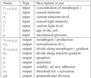
Name Type Description or use
ci,∀i∈[0,2] input concentration of morphogeni
cn input sensed nutrients
n input current nutrients level. cl input sensed light intensity
l input current light level. t input age of the cell p input mechanical pressure oi,∀i∈[0,2] output morphogeni production
oN output normalisation ofoi
di,∀i∈[0,2] output divide along morphogeni gradient
dn output divide along nutrient gradient
a output apoptosis q output quiesence
s output solidify: no new adhesion sT output threshold fors activation
pd output perpendicular division
Table 1: List of our artificial grn inputs and outputs proteins.
newly produced proteins and the destroyed one. More de-tails on the aGRN dynamics can be found in (Cussat-Blanc et al., 2015).
Table 1 describes the configuration of our aGRN input and output proteins when applied to this artificial embryogenesis problem. A few clarifications on the role of some of these in-puts and outin-puts is necessary. First, the sensed nutrients (cn)
input represents the actual concentration in nutrients sensed by the cell in its surrounding environment. The current nu-trients level (n) input is the actual current level of nunu-trients in the protein. The same goes for the light intensity sensed by the cell (cl) and the current amount of light energy
accu-mulated in the cell (l).
The cells express their choices between division, quies-cence or apoptosis through the concentrations of the out-put proteinsdi,a and q respectively. The protein with the
biggest concentration represents the cell’s choice. In ad-dition to starting a division, thedi outputs proteins of the
aGRN also controls the cells’ division plan: eachdi output
protein corresponds to a morphogen, and thedi ordn
pro-tein with maximum concentration is used to determine the gradient (morphogen or nutrient) along which the cell must divide. If no gradient of said morphogen is present, the axis of division is randomly chosen. Thepd protein allows the cell to choose between a division along the morphogen gra-dient or perpendicular to it.
The solidify output proteins controls the solidify capacity of a cell: if the concentration of proteins below the thresh-old proteinsT, the cell then solidifies and will not accept any
more adhesion from not yet connected cells until the concen-tration of proteins decreased under the concentration of sT.
Evolution
One of the goals of this experiment is to explore how ar-tificial multicellular organism could survive in a harsh en-vironment without explicitly leading it to a given strategy or morphology. We wanted to explore the organisms that the rules of this world could create without constraining the creativity of evolution through some restrictive explicit ob-jective function. Therefore, the only obob-jective for the cells is to survive as long as they can, or more precisely, to keep at least one copy of their DNA in our virtual world for as long as possible. While this gives full freedom to the cells on the developmental strategies they can use and on their morphologies (one single cell living on its resources is, for example, an option), it also dramatically increase the search space and fills it with many local optima that pave the way to increased longevity. The first employed approach was to use a standard objective based genetic algorithm (GA). We implemented most features of the Gene Regulatory Net-work Evolution through Augmenting Topology algorithm (GRNEAT) (Cussat-Blanc et al., 2015).
Genetic algorithm
In this algorithm inspired by the NEAT algorithm, the first population of aGRNs is initialized with small topologies (Stanley and Miikkulainen, 2002), containing only input and output proteins. The population is evaluated standardly with a fitness, detailed hereafter, promoting survival time and novelty. After a 3-player tournament selection, offspring are crossed over using a protein alignment operator. This oper-ator uses a genetic distance metric to compute topological distances between two aGRN proteins. Each type of pro-teins is processed separately. Both the input and the output proteins are treated with the same method. One of each in-put (or outin-put) protein linked to a sensor (or an actuator) is randomly selected from one of the parents. The regulatory proteins are then aligned before being crossed: for each reg-ulatory proteinp1
i from the first parent, the closest regulatory
proteinp2
jnot yet aligned is selected from the second parent.
The distance between two proteins is computed as follows:
D(A, B) = 1
p#a|idA− idB| + b|enhA− enhB| + c|inhA− inhB|
$
whereidxis the tag,enhxis the enhancer tag andinhxis
the inhibiter tag of proteinx and p is the precision of the GRN.a, b and c are constants that weight each part of the protein properties, here set up toa = 0.75, b = c = 0.125. If the distance D(p1
i, p2j) is lower than a given alignment
threshold σa, both proteins are aligned. An aligned protein
cannot be aligned anymore. Once alignment of all proteins has been attempted, one protein of each aligned pair is ran-domly selected and added to the offspring. The regulatory proteins that failed to align in both parents are also added to
the offspring. This ensures that no crucial genetic material is deleted during the crossover. Finally, the dynamics coeffi-cients are also crossed. One of the β and the δ coefficoeffi-cients is randomly selected from the parent genomes and used in the offspring genome.
Crossed-over aGRNs represent 30% of the offsprings. The rest of the offsprings are built using tournament selected genomes from the previous generation. All offsprings ex-cept the elite (the best genome) are then subject to mutation with a 75% rate. When mutated, a genome can be modi-fied in three different ways: (1) delete a protein, with a 15% probability, randomly select a regulatory protein, if any, that is removed from the aGRN; (2) add a protein, with a 15% probability, adds a randomly generated regulatory protein; (3) modify a protein, with 70% probability, randomly mod-ify exactly one parameter parameter of the aGRN, either one protein tag or one of the dynamics coefficients.
Novelty metrics
In order to try to mitigate the adverse effects of increased degrees of freedom and numerous local optima in the mor-phological parameter space, we added a novelty metric as defined in (Lehman and Stanley, 2008). We combined this novelty score with our main survival objective through a slight modification of the selection phase of our genetic al-gorithm: each potential parent is selected through a tour-nament based on either novelty or survival time, with a 50% chance. While not as complex as some other inte-grations of novelty in a multi-objective genetic algorithm (Mouret, 2011), this proved sufficient to harness some of the exploratory power of novelty. In this experiment, we tried three different novelty metrics, which are based on the capture (and comparison) of various aspects of a developing phenotype:
• N m0is composed of three numbers: the maximum
num-ber of cells during the simulation, the maximum depth reached by a cell and the total survival time (which is also the main objective).
• N m1 is composed of 5 snapshots of the simulation (at
timest = 10, t = 20, t = 50, t = 75 and t = 100). Each snapshot contains 2 numbers: the number of cells and the maximum depth of a cell at the time of the capture.
• N m2is a set of 5 captures (taken at the same time steps
as forN m1) represented as a20 × 20 integer matrix. It is
actually a set of pictures in which each pixel’s value rep-resents the number of cells stacked. The plane of the shot is determined through a Principal Component Analysis on the cells position (it is the most discriminant plane). This metric is meant to capture the morphologies of the organ-isms in all their subtleties
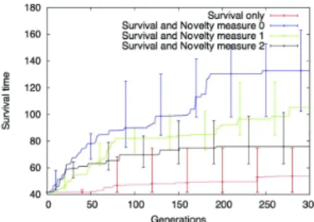
Figure 1: Errorbar plots of the best individuals obtained on 10 independent runs. Errorbars represents the median, the first and third quartiles. All novelty objectives are obviously helping to escape local optimum. However, the novelty mea-sureN m0is giving better results. The initial value of 41
ob-tained at generation 0 represents the survival time for a seed cell that stays quiescent during the whole simulation
Results
Influence of noveltyIn Figure 1, we can see the median (with first and third quar-tile) survival times of the best genomes evolved during 300 generations in 10 independent runs. This graph reveals both the deceptiveness of the fitness landscape when the survival time is used as only fitness objective as well the beneficial impact of novelty. This is undeniable (Student t-test p-values are provided in table 2): where a classical objective based evaluation struggles to find solutions that pass the first local optima (for example: not dividing and surviving on the ini-tial resources of the seed cell, or just doing a few divisions in order for some cells to reach the surface and bring in a little bit of light), the novelty based approaches successfully find solutions to overcome these optima and efficiently pave the way to more robust organisms.
The three novelty measures tested in this experience show that too much information lose the evolution in the search space: the novelty measureN m0globally does better than
both other measures. This measure is the one that includes the fewer parameter. In our opinion, when too much param-eters are used, the exploration is too large and not focus on real novel individuals. Therefore, it is of high importance to wisely choose paratemers that really describe the novelty
Survival N m0 N m1 N m2
Survival - 0.002 0.011 0.089 N m0 0.002 - 0.360 0.050
N m1 0.011 0.360 - 0.250
N m2 0.089 0.050 0.250
-Table 2: p-values of the paired student t-test run comparison between runs with survival fitness and the different novelty measures calculated on 10 runs at generation 300.
of the morphology created by the evolution. As depicted by from table 2, the relatively high p-values between novelty based runs reveal the necessity to make a broader study on the influence of the novelty parameters in order to find the best possible measures for evo-devo models.
Developmental strategies and world setup influence Along all the evolutionary runs, we observed an important diversity of developmental strategies and morphologies, es-pecially when any form of novelty was involved. Figure 2 shows examples of cells arrangements obtained with differ-ent worlds parameters. The distribution of nutridiffer-ents in the world was also found to be of huge influence over the pre-ferred strategies: as expected, large values ofCn andPn
favored a very vertical growth of the cell colony, with the formation of a relatively thick trunk in the ground enabling fast nutrient and light transfer between the deep roots cells and the emerged ones. One of the most interesting results might be the emergence of a form of parthenogenesis when the nutrients concentration was uniform. Cells indeed under-standably found the benefits of a vertical growth to be per-fectly incomparable with the efficiency of a vertical growth. They also adopted, as shown in Figure 2, a spread method where they would laterally develop just below the surface. When a root cell encountered a nutrient source, it would also divide upward (to the surface) and the cells between the two formed cluster would undergo apoptosis, thus cre-ating a simple form of parthenogenesis reminiscent of the biological reproduction of some plants.
Conclusion
In this paper, we have presented a new developmental model based on MecaCell, a physics engine build for artificial life experiments. This developmental model shows how novelty search can help when steping artificial embryogenesis up to the third dimension. Indeed, this added dimension allows for more degrees of freedom for the multicellular organisms but also add a lot of complexity for the cell controller. As a matter of fact, this makes the search space hard to explore with standard fitness function. In addition to the use of a 3D developmental model, we also wanted to remove all engi-neering from the main fitness objective: it is only targets to the survival duration of the organism. By only using this ob-jective, we showed that the evolution is stuck in one or few local optima. By adding different novelty objectives based on the organisms morphologies and capacities to explore its environment, we showed that the evolution can escape from this local optimum and develop more complex morpholo-gies and behaviors able to survive longer in the exact same environment.
This new developmental model opens many research per-spectives. Firstly, we need to study more precisely the in-fluence of the environment parameters on the multicellular organisms. During the development of the presented
exper-Figure 2: Examples of organisms obtained with the different fitnesses. From left to right: survival only and noveltyN m0,1,2.
iment, one of the major difficulty was to produce a viable environment, easy enough to allow the organims to grow but not too hard to produce complex behaviors. Balancing this is complex and need to be studied in detail.
Once done, we want to produce an artificial world in which different organisms would coexist, cooperating or competiting for survival and reproduction. This will require specialization capacities of the cells in order to balance the capacities of the organisms, ones could be good at extracting light energy and other for reproduction. We hope to produce more complex organisms and mimic the early stage of ap-pearence of life on earth
References
Cheney, N., Clune, J., and Lipson, H. (2014). Evolved elec-trophysiological soft robots. In ALIFE 14: The
Four-teenth Conference on the Synthesis and Simulation of Living Systems, volume 14, pages 222–229.
Cussat-Blanc, S., Harrington, K., and Pollack, J. (2015). Gene regulatory network evolution through augment-ing topologies. Evolutionary Computation, IEEE Transactions on, 19(6):823–837.
Disset, J., Cussat-Blanc, S., and Duthen, Y. (2014). Self-organization of symbiotic multicellular structures. In
the Fourteenth International Conference on the Syn-thesis and Simulation of Living Systems-ALIFE 2014, pages pp–541.
Doursat, R. (2009). Organically grown architectures: Creat-ing decentralized, autonomous systems by embryomor-phic engineering. In Organic computing, pages 167– 199. Springer.
Doursat, R. and S´anchez, C. (2014). Growing fine-grained multicellular robots. Soft Robotics, 1(2):110–121.
Fontana, A. and Wr´obel, B. (2013). An artificial lizard regrows its tail (and more): regeneration of 3-dimensional structures with hundreds of thousands of artificial cells. In Advances in Artificial Life, ECAL, volume 12, pages 144–150.
Joachimczak, M., Kowaliw, T., Doursat, R., and Wrobel, B. (2013). Controlling development and chemotaxis of soft-bodied multicellular animats with the same gene regulatory network. In Advances in Artificial Life,
ECAL, volume 12, pages 454–461.
Joachimczak, M. and Wr´obel, B. (2011). Evolution of the morphology and patterning of artificial embryos: scal-ing the tricolour problem to the third dimension.
Ad-vances in artificial life. Darwin meets von Neumann, pages 35–43.
Lehman, J. and Stanley, K. O. (2008). Exploiting open-endedness to solve problems through the search for novelty. In ALIFE, pages 329–336.
Lowengrub, J. S., Frieboes, H. B., Jin, F., Chuang, Y., Li, X., Macklin, P., Wise, S., and Cristini, V. (2009). Nonlinear modelling of cancer: bridging the gap between cells and tumours. Nonlinearity, 23(1):R1.
Mouret, J.-B. (2011). Novelty-based multiobjectivization. In New horizons in evolutionary robotics, pages 139– 154. Springer.
Ouchi, N. B., Glazier, J. A., Rieu, J.-P., Upadhyaya, A., and Sawada, Y. (2003). Improving the realism of the cellular potts model in simulations of biological cells.
Physica A: Statistical Mechanics and its Applications, 329(3):451–458.
Stanley, K. O. and Miikkulainen, R. (2002). Evolving neural networks through augmenting topologies. Evolutionary