HAL Id: hal-00305073
https://hal.archives-ouvertes.fr/hal-00305073
Submitted on 3 May 2007
HAL is a multi-disciplinary open access
archive for the deposit and dissemination of
sci-entific research documents, whether they are
pub-lished or not. The documents may come from
teaching and research institutions in France or
abroad, or from public or private research centers.
L’archive ouverte pluridisciplinaire HAL, est
destinée au dépôt et à la diffusion de documents
scientifiques de niveau recherche, publiés ou non,
émanant des établissements d’enseignement et de
recherche français ou étrangers, des laboratoires
publics ou privés.
hydrological ensemble forecasting of the Laurentian
Great Lakes at the regional scale
A. Pietroniro, V. Fortin, N. Kouwen, C. Neal, R. Turcotte, B. Davison, D.
Verseghy, E. D. Soulis, R. Caldwell, N. Evora, et al.
To cite this version:
A. Pietroniro, V. Fortin, N. Kouwen, C. Neal, R. Turcotte, et al.. Development of the MESH modelling
system for hydrological ensemble forecasting of the Laurentian Great Lakes at the regional scale.
Hydrology and Earth System Sciences Discussions, European Geosciences Union, 2007, 11 (4),
pp.1279-1294. �hal-00305073�
www.hydrol-earth-syst-sci.net/11/1279/2007/ © Author(s) 2007. This work is licensed under a Creative Commons License.
Earth System
Sciences
Development of the MESH modelling system for hydrological
ensemble forecasting of the Laurentian Great Lakes at the
regional scale
A. Pietroniro1, V. Fortin2, N. Kouwen3, C. Neal4, R. Turcotte5, B. Davison6, D. Verseghy7, E. D. Soulis3, R. Caldwell8, N. Evora9, and P. Pellerin2
1Water Science and Technology Directorate, Environment Canada, National Hydrology Research Center, Saskatoon SK
Canada S7N 3H5, Canada
2Recherche en Pr´evision Num´erique, Meteorological Research Division, Environment Canada, Canadian Meteorological
Center Dorval QC Canada H9P 1J3, Canada
3Department of Civil Engineering, University of Waterloo, Waterloo ON Canada N2L 3G1, Canada
4Hydrological Applications and Services, Meteorological Service of Canada, Ottawa ON Canada K1N 1A1, Canada 5Centre d’expertise hydrique du Qu´ebec, Minist`ere du D´eveloppement durable, de l’Environnement et des Parcs,
Gouvernement du Qu´ebec Quebec City QC Canada G1R 5V7, Canada
6Hydrometeorology and Arctic Laboratory, Meteorological Service of Canada, National Hydrology Research Center,
Saskatoon SK Canada S7N 3H5, Canada
7Climate Research Division, Environment Canada, Toronto ON Canada M3H 5T4, Canada
8Great Lakes – St. Lawrence Regulation Office, Meteorological Service of Canada, Cornwall ON Canada K6H 6S2, Canada 9Institut de recherche d’Hydro-Qu´ebec, Varennes QC Canada J3X 1S1, Canada
Received: 31 May 2006 – Published in Hydrol. Earth Syst. Sci. Discuss.: 29 August 2006 Revised: 16 January 2007 – Accepted: 26 March 2007 – Published: 3 May 2007
Abstract. Environment Canada has been developing a
com-munity environmental modelling system (Mod´elisation En-vironmentale Communautaire – MEC), which is designed to facilitate coupling between models focusing on different components of the earth system. The ultimate objective of MEC is to use the coupled models to produce operational forecasts. MESH (MEC – Surface and Hydrology), a con-figuration of MEC currently under development, is special-ized for coupled land-surface and hydrological models. To determine the specific requirements for MESH, its differ-ent compondiffer-ents were implemdiffer-ented on the Laurdiffer-entian Great Lakes watershed, situated on the Canada-US border. This ex-periment showed that MESH can help us better understand the behaviour of different land-surface models, test differ-ent schemes for producing ensemble streamflow forecasts, and provide a means of sharing the data, the models and the results with collaborators and end-users. This modelling framework is at the heart of a testbed proposal for the Hy-drologic Ensemble Prediction Experiment (HEPEX) which should allow us to make use of the North American En-semble Forecasting System (NAEFS) to improve streamflow
Correspondence to: A. Pietroniro
forecasts of the Great Lakes tributaries, and demonstrate how MESH can contribute to a Community Hydrologic Predic-tion System (CHPS).
1 Introduction
There is an intensive global research effort to couple at-mospheric and hydrological models to improve hydrological flow simulations and atmospheric predictions in both climate (Soulis et al., 2000) and weather prediction models (Benoit et al., 2000). The land surface is an important hydrological control because of its primary influence on the surface water budget. Sophisticated soil-vegetation atmospheric transfer schemes (SVATs) are currently being implemented in global climate models, regional climate models and day-to-day op-erational forecasting numerical weather prediction (NWP) models. However, SVATs have rarely been incorporated into hydrological models. Over the last 10 years, there has been a systematic attempt, through collaborative research in Canada and under a variety of research programs, to couple atmo-spheric and hydrological models using SVATs as the mon link (Soulis et al., 2005). Our approach has been to com-bine different SVATs and hydrological streamflow models
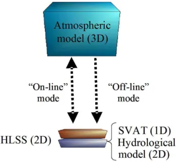
Fig. 1. A strategy for coupled atmosphere, land and hydrology
mod-els.
to provide a suite of stand-alone hydrology-land-surface schemes (HLSS). These stand-alone models are now being incorporated into the atmospheric models, creating a fully coupled system. The flexibility of this system permits the analysis of the HLSS’ sensitivities to parameterization and physical conceptualizations, and assesses the models’ impact on hydrological and atmospheric prediction. Nonetheless, while these efforts have led to the development of models that are suitable for research purposes, their use in hydrometeoro-logical forecasting systems has been limited. This is largely a result of the technical hurdles involved in testing changes to an operational NWP system. To help bridge the gap between research and operations in surface modelling, the numerical weather prediction research group at Environment Canada (RPN) has developed a community environmental modelling system called MEC. The MEC system allows different sur-face models to coexist within the same modelling framework so that they can easily be compared for the same experi-ment using exactly the same forcings, interpolation proce-dures, grid, time period, time step and output specifications. Furthermore, MEC is designed to facilitate coupling between models which focus on different components of the earth sys-tem with the objective of using the coupled models to pro-duce operational forecasts. The model coupler, developed jointly with the Centre Europ´een de Recherche et de For-mation Avanc´ee en Calcul Scientifique (CERFACS), can be used to couple models running on different grids, and po-tentially, on different time steps (Pellerin et al., 2004; Val-cke et al., 2004). An important feature of MEC is its abil-ity to read atmospheric forcings from files instead of obtain-ing them from an atmospheric model through the coupler.
This makes it possible to test changes to the surface schemes offline. This is the approach used in this study: MEC was forced using atmospheric fields generated by different mod-els to obtain simulations and ensemble forecasts of surface and hydrological variables.
The current version of MEC includes three land-surface schemes: (1) a simple force-restore scheme; (2) a version of the ISBA scheme (Interaction Soil-Biosph`ere-Atmosph`ere, Noilhan and Planton, 1989; B´elair et al., 2003a,b); and (3) version 3.0 of the Canadian Land Surface Scheme (CLASS) (Verseghy, 2000). MESH, a configuration of MEC cur-rently under development, includes, in addition to the land surface models available in MEC, the land-surface parame-terization and hydrological routing schemes used by WAT-FLOOD (Kouwen et al., 1993). Furthermore, in MESH, the land surface model CLASS can run on a number of different tiles on each grid cell, which allows the subgrid variability in the landscape to be taken into account. Using the grouped-response unit (GRU) approach, a parameter set is identified for each landscape class so that the calibration of the model is not done at the grid cell level nor at the sub-basin level, but on the whole domain at once.
The MESH regional hydrological model was calibrated on the St. Lawrence River basin at Montr´eal, which includes all of the Laurentian Great Lakes plus all of the Ottawa River basin. In this paper, we show how this model can be used to obtain simulations and ensemble forecasts of both surface variables and streamflow, which can be useful for managing the waters of the Great Lakes. The emphasis is to illustrate the potential of the technology currently available at Envi-ronment Canada: all of the observations that are used for running the model, and all of the pieces of software used in this study are readily available to produce the simulations and the ensemble forecasts in real-time.
The paper is organized as follows. Following the Intro-duction in Sect. 1, in Sect. 2 we discuss the design of the MESH system in greater detail . In Sect. 3, we present the existing modelling and forecasting capabilities for the Great Lakes basin, and discuss how a regional hydrometeorologi-cal modelling and ensemble forecasting system can help im-prove water resources management in this basin. In Sect. 4, we present the atmospheric forcings used to obtain simula-tions and ensemble forecasts of the snow water equivalent (SWE), of streamflow in each sub-basin and of lake inflows. In Sect. 5, we present the model setup and the calibration technique. In Sect. 6, we present and discuss the results of the streamflow and lake inflow simulation and forecast. In Sect. 7, we present results for the SWE simulation and semble forecasting, and discuss how we can obtain an en-semble of initial snow conditions for the hydrological model. A brief conclusion follows in Sect. 8.
2 Design of the MESH system
The MEC and MESH systems were developed by Environ-ment Canada to optimize research and developEnviron-ment (R&D) in environmental modelling and to bridge the gap between R&D and operations by allowing researchers in different communities, as well as end-users, to share a unified mod-elling environment. MESH is a HLSS built from the MEC system which uses a mosaic approach for runoff routing and more detailed land-surface modelling.
2.1 Online and offline hydrological modelling
MEC is essentially a generic model driver for a 1-D surface model which has the additional capability to pass 2-D fields back and forth between models such as atmospheric or hy-drological models. MESH is a configuration of MEC that is specialized for coupled land-surface and hydrological mod-elling. As shown by Fig. 1, the land-surface and hydrological models are tightly integrated, running on the same grid. The land-surface model can then be coupled to an atmospheric model through the coupler (the online mode), or MEC can read atmospheric forcings in from files (the offline mode). Our streamflow and SWE simulations were performed of-fline using gridded hourly precipitation and temperature data derived from all available synoptic stations within the region. In both cases, the atmospheric forcings can be provided on a different grid and at different time intervals. For land-surface modelling, we can take advantage of this capability and run the surface model at a higher resolution because the com-puter resources needed to run a land-surface model are typi-cally much less than for an atmospheric model.
2.2 Resolving the subgrid variability in geophysical fields Running MEC at a higher resolution than the atmospheric forcings can be useful to better resolve the heterogeneity in the geophysical fields (such as land cover and soil texture). It also allows us to adapt the atmospheric forcings to take into account the change in resolution. For example, the temper-ature and precipitation phase can be adapted to account for the difference in elevation between the topography seen by the atmospheric model and the topography seen by MEC, as the topography seen by the atmospheric model is typically smoother than the MEC topography.
Often, we are only interested in obtaining aggregated fluxes and variables which encompass the heterogeneity in the geophysical fields, and not in high-resolution simula-tions. This is typically the case for regional hydrological modelling, where we want a spatial resolution sufficient to resolve first-order watersheds, but must also account for the heterogeneity in land cover and soil texture to obtain accurate simulations of surface variables. In this case, from a compu-tational point of view, it makes more sense to run the surface model in mosaic mode.
2.3 The tile connector and the grid connector
In mosaic mode, which is the typical setup for MESH, each grid cell is subdivided into a number of tiles and the land-surface model is run on each tile independently. After all tiles have been run, an aggregation step is performed to ob-tain overall fluxes and prognostic variables for each grid cell, an operation effected by a tile connector. At the moment, the tile connector only takes a weighted average of the fluxes and of the prognostic variables, but it has the potential to allow tiles to interact with one another. For example, snow could blow from open areas to forested areas within a grid cell. Energy and mass can move from one grid cell to the next through the grid connector. When running offline, the cur-rent MESH grid connector simply routes the surface runoff, interflow and drainage generated at each grid cell by the land-surface scheme through a river network, accounting for long-term storage of water in the watershed through a conceptual reservoir.
2.4 Parallel computing
Finally, we note that because it takes advantage of the 1– D nature of land-surface schemes, MEC can run very effi-ciently on clusters. The domain is divided into subareas and the land-surface model is run independently on each area. At the end of each time step, after the land surface model has finished running on each node, only the 2-D fields that need to be shared with other models are sent back to a single pro-cessor. The processor then calls the 2-D models and sends the appropriate fields to the coupler when running in online mode. In MESH mode, the routing model is run through a subroutine call, since it runs on the same grid as the land-surface model, and interaction with other models (such as an atmospheric or a groundwater model) is accomplished through the coupler. Algo. 1 summarizes how MESH han-dles the time-stepping loop.
3 The Great Lakes basin
The Great Lakes basin, straddling the Canada-US border (cf. Fig. 2), contains approximately 20% of the world’s fresh surface water supply. The watershed area is approximately 1 million square kilometers and close to 40 million people live within it, including roughly one-third of the population of Canada (Gov. of Canada and EPA (1995)). Water empties from the Great Lakes at the outlet of Lake Ontario, the last of the five Great Lakes into the St. Lawrence River and passes through the Moses-Saunders dam. Before reaching the Mon-treal archipelago, which is immediately downstream of its confluence with the Ottawa River, the St. Lawrence River is also fed by a number of rivers originating in the Adirondacks (New York State).
Algorithm 1 MESH time-stepping algorithm
1: Initialize all prognostic variables and parameters 2: for each time step do
3: {These computations can be distributed on different comput-ing nodes. Internal prognostic variables of the surface model need not be shared between computing nodes}
4: for each grid cell do
5: for each tile on a given grid cell do
6: Run the 1-D surface model for one time step and one tile
7: end for
8: Tile connector: aggregate results for each tile
9: end for
10: {These computations are performed on a single processor, which however needs to access only a limited number of variables}
11: Obtain from each computing node the 2-D fields necessary for the grid connector and the coupler
12: Grid connector: route runoff, interflow and drainage
com-puted on each grid cell through the river network for one time step
13: if the coupler is used then
14: send 2-D fields required by the coupler for other models 15: wait for the coupler to provide 2-D fields required by
MESH
16: end if
17: end for
Fig. 2. The Great Lakes and St. Lawrence basins upstream of
Montr´eal, with the Ottawa River basin shown in gray and the provincial and international boundaries shown in black.
3.1 Water management on the Great Lakes basin
Water levels in the Great Lakes are regulated according to an international agreement between Canada and the United States which is under the responsibility of the International Joint Commission (IJC) and is overseen by the International Lake Superior Board of Control (ILSBC) for Lake Superior, and the International St. Lawrence River Board of Control (ISLRBC) for Lake Ontario and for the St. Lawrence.
Out-flow from the other lakes (Huron, Michigan, Erie) is unregu-lated. According to the ISLRBC web site:
“One requirement in the Commission’s order was to regu-late Lake Ontario within a target range from 74.2 to 75.4 me-tres (...) above sea level. The project must also be operated to provide no less protection for navigation and shoreline interests downstream than would exist without the project. (...) When supplies exceed those of the past, shoreline prop-erty owners upstream and downstream are to be given all possible relief. When water supplies are less than those of the past, all possible relief is to be provided to navigation and power interests. (...) Experience has shown that during spring runoff from the Ottawa River, a major tributary, flood-ing in the Montreal area has been reduced by temporary Lake Ontario outflow reductions.”
Lake Ontario outflow strategies are typically based on lake levels, forecasted inflows to the lake and forecasted outflows from the St. Lawrence and Ottawa River basins for the fol-lowing weeks, and thus may benefit from better ensemble streamflow forecasts both of Lake Ontario inflows and Ot-tawa River flow for the first 15 days. In particular, a use-ful product would be a joint ensemble forecast of inflow to Lake Ontario, of river flow into the St. Lawrence between the Moses-Saunders dam and the Montreal archipelago and of Ottawa River flow. However, because many of the sub-basins on the Ottawa River are regulated, such a product could only be obtained after careful modelling of reservoir operations. 3.2 Water management on the Ottawa River subbasin The Ottawa River is the chief tributary of the Saint Lawrence River. It rises from its source in Lake Capimitchigama in western Quebec and then runs for 1271 km before merging with the Saint Lawrence River at Montreal. Its drainage area has a size of 146 000 km2and its mean flow is on the order of 2000 m3/s. The integrated water management on the Ottawa River basin provides protection against flooding along this river and its tributaries and also insures hydroelectric produc-tion by various users (Hydro-Quebec, Ontario Power Gen-eration and the Ministry of Sustainable Development, Envi-ronment and Parks of Quebec). In March 1983, the Gov-ernments of Canada, Ontario and Quebec agreed to consti-tute the Ottawa River Regulation Planning Board (ORRB), which consists of seven members, Hydro-Quebec being one of them. The Ottawa River Regulating Committee (ORRC) is the operational arm of the Board. ORRC formulates and review periodically regulation policies and criteria leading to integrated management of the principal reservoirs.
Hydro-Quebec operates 12 hydroelectric generating sta-tions and 3 reservoirs (Dozois, Cabonga and Baskatong) on the Ottawa River basin. These generating stations are mostly run-of-river stations with an installed capacity of about 1850 MW. Carillon is the most powerful generating station (752 MW). The Cabonga and Baskatong reservoirs are located in the Gatineau River basin. The Gatineau River,
which is a major tributary of the Ottawa River with a basin of about 24 000 km2, flows through the communities of Mani-waki, Wakefield, Chelsea and Gatineau. The management of these reservoirs is very important to prevent or limit the flooding of these communities.
3.3 Existing forecasting capabilities
Given the socio-economic importance of the watershed, there are of course, existing hydrological forecasting tools for many rivers in the basin. The Great Lakes Environmental Research Laboratory (GLERL) already provides 48 h deter-ministic forecasts of the Great Lakes’ water levels through the Great Lakes Coastal Forecasting System (GLCFS) and monthly forecasts of lake inflows and water levels through its Advanced Hydrologic Prediction System (AHPS), which are updated daily1. The ORRB provides a 13-week outflow forecast for the Ottawa River routinely on a weekly basis and on a daily basis when required. Ensemble streamflow pre-dictions based on a deterministic weather forecast are issued daily by Hydro-Qu´ebec for many sub-watersheds of the Ot-tawa River. For the purpose of preventing or limiting flood-ing on the Gatineau River, Hydro-Qu´ebec also issues reser-voir inflow and streamflow forecasts using the distributed hy-drological model HYDROTEL (Fortin et al., 2001) forced by a deterministic atmospheric forecast and by meteorological scenarios representing the uncertainty on this forecast. To our knowledge, none of these systems use ensemble meteo-rological forecasts.
3.4 Ensemble-based hydrological products of interest for the Great-Lakes
From among hydrological ensemble products that could be provided by MESH using the Canadian Ensemble Prediction System (EPS), we decided to investigate: (1) streamflows for the unregulated sub-watersheds upstream of the Moses-Saunders dam, (2) lake inflows into Lake Ontario, and (3) snow water equivalent (SWE). Given the large amount of regulation within the Great Lakes basin and on the Ottawa River basin, the production of ensemble SWE forecasts ap-peared to be a useful product to assist water managers who already have forecasting capabilities that make use of snow water equivalent estimations for forecasting streamflow dur-ing snowmelt events.
4 Atmospheric forcings
4.1 Forcings available for simulation purposes
In order to obtain ensemble forecasts of surface and hydro-logical variables, it is necessary to spin up the surface and
1Lake Ontario levels are actually not forecasted by the GLERL,
but rather computed by Environment Canada monthly using infor-mation provided by GLERL.
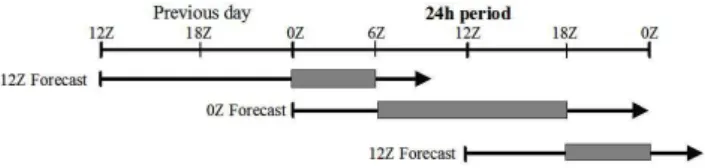
Fig. 3. Building a continuous time-series of atmospheric forcing
from short-term forecasts.
hydrological models to allow them to reach a state that is reasonably consistent with observed data before forcing them with output from an EPS. While the land surface parameter-ization associated with WATFLOOD only requires tempera-ture and precipitation observations, the land surface schemes ISBA and CLASS also require pressure, wind speed, humid-ity and incoming radiative forcings (long-wave and short-wave).
Although precipitation observations can be interpolated to obtain a precipitation field if there are enough gauges report-ing in real-time, this is not possible for radiative forcreport-ings. We hence decided to rely on a short-term forecast. Since June 2004, the Meteorological Service of Canada (MSC) has is-sued a meteorological forecast each day at 0 h and 12 h UTC out to 48 h on a 15 km grid using the Global Environmental Multiscale (GEM) model (Cˆot´e et al. (1998)) in its regional configuration (Mailhot et al., 2005). Between October 2001 and June 2004, the same model was run on a 24 km grid, generating a 5-year archive of short-term forecasts of all the atmospheric variables required to run ISBA and CLASS. Of course, this forecast is more accurate for shorter lead times, but because GEM also needs some spin-up time, the quality of the precipitation fields appears to be better for lead times of 6 h to 18 h (Mahfouf et al. (2005)).
To obtain atmospheric forcings that are coherent with one another, we created a continuous time series of the atmo-spheric forcings required by ISBA and CLASS by combin-ing all of the forecasts issued since October 2001 with lead times of 06:00 h to 18:00 h. This is sufficient because there are two forecasts issued each day. This means that: (1) the forcings valid from 00:00 h to 06:00 h UTC each day were obtained from the forecast issued at 12:00 h UTC the previ-ous day (with lead times between 12:00 h and 18:00 h); (2) the forcings valid from 06:00 h to 18:00 h UTC each day were obtained from the forecast issued at 00:00 h UTC the same day (with lead times of 06:00 h to 18:00 h); and (3) the forcings valid from 18:00 h to 00:00 h UTC the next day were obtained from the forecast issued at 12:00 h UTC that day (with lead times of 06:00 h to 12:00 h). This process is illustrated by Fig. 3. Because precipitation is so difficult to forecast, even for short lead times, we can also use ob-servations at synoptic stations to force the surface models. Observations were quality controlled and gridded using or-dinary kriging (Matheron, G., 1963). We note that to further
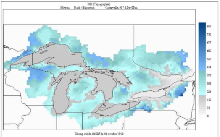
Fig. 4. Topography of the basin at 1/6th of a degree
improve the precipitation field, it would be useful to merge surface observations, a short-term precipitation forecast and remote sensing observations (including ground-based radar and GOES imagery) in a precipitation analysis, but such a product has yet to be developed in Canada. An experimen-tal high-resolution precipitation analysis is available which combines precipitation observations with a first guess pro-vided by the GEM model using the optimal interpolation technique (Mahfouf et al., 2005). This product is known as CaPA, for Canadian Precipitation Analysis.
4.2 Forcings available for ensemble forecasting purposes Ensemble forecasting was proposed in the early 1990s as a method for describing the uncertainties inherent in NWP modelling. The basic approach is to run the NWP model many times, each time starting from a slightly different ini-tial state and/or a slightly different version of the model. The changes to the initial state (called “perturbations”) are de-signed so as to be within the range of possible true initial states at any particular time. The changes to the model may be in the form of perturbations to the model parameters, also set within the range of possible values, or the model uncer-tainty may be accounted for by using significantly different versions of the model. Some ensembles are made up of com-pletely different models; these are called “multi-model en-sembles”. When a single NWP model is run, it produces forecasts of weather variables such as temperature, pressure, wind and precipitation that are valid for all forecast projec-tions, on a regular grid of points. An ensemble prediction system produces one such forecast, called a member, for each run of the model. Since 1 January 2006, MSC has provided ensemble forecasts for the next 15 days using a multi-model ensemble consisting of two different models, each run in eight different configurations, for a total of 16 members, each starting from different initial conditions representing the un-certainty in the analysis (Pellerin, G., 2003; Houtekamer et al., 2005). A control run is also available, which runs using
the best estimate of the initial conditions. Since ensemble systems comprise many model runs, they require consider-able computer resources to run. To partially compensate for this, and to facilitate the availability of forecasts within a rea-sonable time, the model is usually run at lower resolution, that is, with grid points spaced further apart than the deter-ministic forecast. The current Canadian EPS has about 130 km spacing between points.
Most of the results shown in this paper, however, are gen-erated from a different configuration of the EPS, operational since 1999. Its spatial resolution is the same, but the lead time is only 10 days and each member is configured dif-ferently. This means that the characteristics of the ensem-ble members, in terms of bias or spread for example, have changed recently, and it is therefore not possible to arrive at definitive conclusions concerning the quality of the ensem-ble forecasts from the present study. At the moment, such conclusions cannot be reached by simply testing with output from the new system, because the archive would be too short for this purpose. The validation process can only be acceler-ated through a reforecasting experiment. It should be noted that the Canadian EPS will soon be included in the North American Ensemble Forecasting System (NAEFS), which will combine the EPS of the MSC with the EPS of the US National Weather Service (Toth et al., 2006).
5 Model setup and parameterization
5.1 Spatial and temporal resolution
In order to resolve the sub-watersheds where we wanted to simulate and forecast streamflow, as well as to capture the spatial variability of the precipitation field, we decided to set up MESH at a resolution of 1/6th of a degree. This is sufficient because sub-grid variability in land cover and soil texture can still be taken into account using the mosaic ap-proach. Fig. 4 shows the topography of the basin as seen by MESH at 1/6th of a degree. While it would be relatively easy to increase the spatial resolution of the land-surface model so as to explicitly resolve the variability in land cover and soil texture, it is always difficult to obtain coherent drainage directions, which make it very time-consuming to increase the resolution of the hydrological model. Furthermore, the assumptions made in the hydrological model with respect to routing are scale-dependent, in that they require that a stream exists in every grid cell. Although better results might be ob-tained on individual subwatersheds by increasing the spatial resolution, we consider a resolution of 1/6th of a degree to be a good compromise for a hydrological model covering all of the Great Lakes watershed.
5.2 Setup of the land-surface models
The ISBA and CLASS SVATs are parameterized using a database of vegetation type and soil texture. The vegetation
type used by ISBA and CLASS over North America comes from a United States Geological Survey (USGS) climatologi-cal database on a 1 km by 1 km grid. It includes 24 vegetation types. Vegetation characteristics such as leaf area index, veg-etation fraction and root depth change from day to day in the model according to a pre-established table. These a priori es-timates of parameters are based on a number of years of test-ing and evaluation in the Canadian version of the ISBA land-surface scheme. Since a vegetation climatology is used, the actual vegetation conditions may not match those seen by the model. For soil texture, we use the STATSGO database for the US portion of the basin and the CanSIS database for the Canadian portion of the basin. No calibration is performed for these two models.
5.3 Setup of the hydrological and routing models
The MESH design allows the testing of different combina-tions of land-surface models and routing models in hydro-logical modelling. Nonetheless, the most efficient scheme for constructing a hydrological model is to establish it us-ing a simpler water-balance modellus-ing approach as the land-surface model, to ensure that the hydrological model pro-duces reasonable simulations. It is subsequently easier to test more complex land-surface schemes knowing that the rout-ing model generates the right volume of water, on average, for each sub watershed. Furthermore, for operational pur-poses, it is useful to have a simpler hydrological model that can run faster and with less inputs. This is why we chose to use the simpler WATFLOOD water balance model for this first test of the MESH system, when setting up the routing model. The routing component of MESH is based on the original scheme incorporated in WATFLOOD and requires the topography of the watershed be outlined. The internal physiographic features required for the vertical water budget and grid routing routines such as contour density, drainage direction, channel elevations and land-cover are parameter-ized for each grid. These physiographic parameters are es-sential for describing the horizontal transfer (within tile) and routing (between grids) of water in the model, required for each of the grid elements.
As described above, the surface vertical water budget is independent of the land-surface model which is used in MESH. Indeed, the main design choice in setting up MESH for a basin is the identification of Grouped Response Units (GRUs). As is usually the case, each GRU in this study was set to correspond to a different land cover class. Since the inception of the GRU-approach (Kouwen et al., 1993), it has been possible to successfully calibrate a number of mod-eling applications using a landscape based parametrization. The original treatment of land-covers by WATFLOOD, and subsequently by MESH, is a balance between maximizing the detail associated with physically based modelling and limiting the inevitable complexity that comes with the de-tail. Hydrologic simulation often requires breaking the
wa-tershed down into smaller units to more closely represent the observed hydrological and hydraulic phenomena. Semi-distributed or Semi-distributed approaches to basin segmentation are defined by their ability to incorporate the distributed na-ture of watershed parameters and inputs into a modeling framework. As noted by Pietroniro and Soulis (2003), fully distributed models apply detailed physics in differential form but are too complex and data intensive to solve for large basins. Lumped hydrological models often lack the detail of physics and distributed inputs. A more suitable approach for large basins is the GRU, which is a grouping of all ar-eas with a similar land cover (or other attributes) such that a grid square contains a limited number of distinct GRUs. Runoff generated from each of the different groups of GRUs is then summed and routed to the stream and river systems. In MESH, two GRUs with the same percentages of land cover types, rainfall, and initial conditions produce the same amount of runoff regardless of how these land cover classes are distributed. The major advantage of the GRU approach is that it can incorporate the necessary physics while retaining simplicity of operation.
The surface water budget in WATFLOOD is computed for each GRU within a grid square and infiltrated using the well known Green-Ampt approach. When the infiltration capacity is exceeded by the water supply, and the depression storage has been satisfied, the model then computes overland flow from the Manning equation. Infiltrated water is stored in a soil reservoir referred to as the upper zone storage (UZS). Water within this layer percolates downward or is exfiltrated to nearby water-courses using simple storage-discharge rela-tionships. All GRUs within a grid contribute to the shared lower zone storage (LZS). Ground water, or LZS, is replen-ished by recharge from the UZS according to a power func-tion. A ground water depletion function is used to gradually diminish the base flow. There is only one LZS for each grid. Flow rates through soil depend upon the hydraulic conduc-tivity that is optimized on the basis of land cover. The total inflow to the river system is determined by adding the sur-face runoff and interflow from all GRUs in a grid and the base flow. Total grid flow is added to the channel flow from upstream grids and routed through the grid to the next down-stream grid using a surrogate channel system with a storage routing technique. The GRU-parameter adjustment process is most often done manually. To properly calibrate the model, it is desirable to include as many flow stations as possible in a single model. Ideally, the land cover characteristics of the watersheds will vary such that each chosen land cover dom-inates in some part of the domain. In this way, parameter values for a particular land cover class are fitted to the results in watersheds where that class is the dominant component.
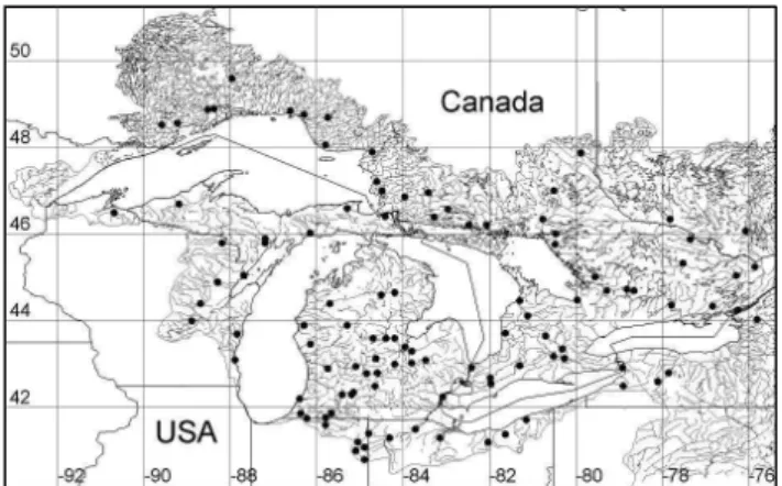
Substantial effort was required to adjust the gridded water-shed map automatically generated by WATFLOOD to match the actual drainage areas for the streamflow gauges shown in Fig. 5. The grid box area is approximately 240 km2while the modelled watersheds ranged from 386 km2 to 16 332 km2.
Fig. 5. Streamflow gauge network used for model calibration and
validation.
The smaller watersheds are used to adjust local routing pa-rameters while the larger watersheds are used to set the river routing parameters.
As previously stated, few changes were made to the pa-rameter sets previously used with WATFLOOD. However, because WATFLOOD currently lacks a lake evaporation model, monthly climatic values provided by GLERL were used for this purpose.
6 Streamflow simulation and forecast
6.1 Operationalizing WATFLOOD
Operationalizing the WATFLOOD model within MESH re-quires a physiographic database derived from two main sources: a digital elevation model and observed land-cover data. The WATFLOOD routing model requires the determi-nation of contour density, channel elevations, drainage direc-tion and grid contributing area for each of the grids. Obtain-ing this information is a fairly objective procedure and has been described extensively by Shaw et al.+ (2005). Man-ning roughness coefficients for the storage-routing between grids are based on river class identifications determined dur-ing model implementation and can be defined a priori or through model optimization. An example of the drainage di-rection and channel elevation derived from the basin digital elevation model (DEM) is shown in Fig. 6.
Additional operational parameters include land-cover characteristics, reservoir and channel properties. The land cover types selected for the Great Lakes basin are crops, grass, deciduous forest, coniferous forest, mixed forest and water. All of these land cover classes have been used in other WATFLOOD model testing at much smaller scales and dif-ferent locations. The land-based parameters required mini-mal change for use with the entire Great Lakes basin. The base temperature for the degree-hour snow model, based on
Anderson’s degree-day method (Anderson, 1973), needed slight adjustment. The major change in this WATFLOOD application was in designating river classes. To properly rep-resent the geomorphology of the rivers in the Great Lakes watershed, five classes were needed: one class for the major connecting links of the lakes; another for the area north of the Great Lakes with the exception of Southern Ontario; a third for the area just south of Lake Superior; a fourth for Northern Michigan and Wisconsin; and one more for the agricultural areas in Southern Ontario, Michigan and Ohio.
Large lakes and reservoirs that can be resolved at the op-erational grid scale are treated as one unit in the model. An outlet for these features must be defined and an outflow hy-drograph or rating curve must be prescribed. In our case simple regression equations developed by the Coordinating Committee on Great Lakes Basic Hydraulic and Hydrologic Data were used for routing water between the large lakes. For lakes Superior, Erie and Ontario, simple power functions were used (cf. Eq. 1).
Q = a · (H − H0)b (1)
In Eq. (1), Q is the lake outflow, H is the lake level, H0is
the datum, and finally a and b are fitted coefficients. In the case of lakes Superior and Ontario, pre-project rela-tionships representing the unregulated case were employed. For the remainder of the lakes, relationships representing the present state were used. For lakes Huron-Michigan and St Clair the function was modified to take into account backwa-ter from the downstream lake:
Q = a · (H − H0)b·(H − HD)c (2) where HDis the level of the lake downstream and c is a fitted coefficient.
In addition, seasonal corrections for weed growth and ice cover were made to the computed flows. A small adjustment was made for Lake Ontario due to the gradual rise of its outlet due to glacial uplift. Simple power functions were also used for the smaller lakes Nipigon and Nipissing. Lake Nipigon is heavily regulated. The lake storages for the MESH routing sheme are shown in Fig. 7.
6.2 WATFLOOD Model Application
The WATFLOOD model was used to simulate streamflow and lake inflows. The study duration was from 1 Novem-ber 2000 to 31 August 2003 inclusive, and streamflow sim-ulations were compared at all streamflow locations shown in Fig. 5. Atmospheric forcing was derived from observed syn-optic stations within the basin, and was interpolated using simple inverse distance weighting functions. As previously discussed, only hourly precipitation and temperature are re-quired to drive the model. In order to initiate the model and determine the initial states of the LZS and UZS, the model was spun-up for a 9 year period using the study time period for 3 continuous runs.
Fig. 6. WATFLOOD Model Domain showing elevation and drainage direction used as part of the physiograhic parametrization fo MESH.
Fig. 7. Large lakes and reservoirs used in the MESH routing
scheme.
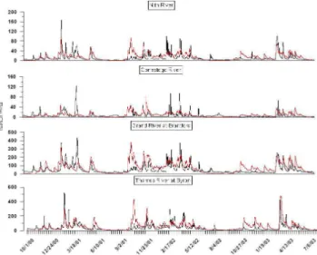
In many cases, deterministic runs using the synoptic forc-ing proved quite reliable. There was no attempt to try to simulate the multitude of controls and diversions within the basin in any systematic way. Only the rating curves described earlier for the 7 reaches identified in Fig. 7 were coded into the routing algorithm. A total of 155 stations were used for comparison. For illustrative purposes, hydrograph compar-isons for four stations located in southern Ontario are shown in Fig. 8. The overall simulations look quite reasonable how-ever there are certainly peak flows that are not captured in the individual gauge simulations. Also evident in Fig. 8 are the spring flows in 2001 where simulated peaks are higher than observed peaks. In some other locations, the oppo-site occurred. This may be due to the fact that small con-trol structures are not accounted for when we operate the model at the scale and resolution we have developed in this
Fig. 8. WATFLOOD model results for selected southern Ontario
basins. Red lines are the simulated hydrographs, black lines are the observed.
study. Of course there are many other issues such as un-certainties in observed precipitation and model uncertainty that need to be examined. What is encouraging is that we were able to achieve reasonable hydrograph simulation at a regional scale for a number of locations. Further investiga-tion is still required and will be conducted in a systematic way as we continue to develop the system. Presently, we find that these large scale simulations are executed at at a suffi-cient resolution allowing us to determine specific geographic areas of concern where the system is failing. In conjucntion with the flow analysis, we also made analyzed total inflows
Fig. 9. Lake level estimates for the study time period estimates
using WATFLOOD and MESH modelling system.
into each of the Great Lakes. As mentioned, the Lakes were treated as individual reaches and all of the routed runoff from upstream rivers is summed and added for the reach at ev-ery time step. Using the rating curves for lake routing, the following simulations of Great Lakes water levels were ob-tained (see Fig. 9). Clearly, though some issues require res-olution, the general patterns and seasonality of the lake lev-els for all five Great Lakes are well simulated. It should be noted that lake evaporation is based on climatological esti-mates derived from GLERL, and that precipitation over lakes is based solely upon the synoptic observations interpolated for the MESH domain. This may explain some of the varia-tions observed in the model as compared to observavaria-tions. It should be also noted that Lake Ontario has some measure of regulation that has not been accounted for in this model. The discrepancies in Lake Superior are more problematic and will require further attention.
Ensemble runs were performed primarily as a proof-of-concept to demonstrate the potential of the MESH modelling system at the regional scale. Inflows into Lake Ontario, and the resulting lake level, are particularly important for down-stream infrastructure, such as the Port of Montreal. Although the deterministic model ran for the entire study period for the
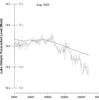
Fig. 10. Deterministic lake level estimates from the WATFLOOD
simulation for August 2003. The grey solid lines represent mea-sured lake levels, the dashed grey line is the 5-day moving average. The black line is the WATFLOOD simulation.
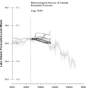
ensembles, the deterministic runs were completed to the end of July and provided the initial conditions for the ensemble runs for August. On 1 August, simulations were made using the 10-day ensemble forecast for precipitation and temper-ature. The following day, 2 August, the synoptic forcings were used for August 1 and the ensemble forecast was used for 2 August and the subsequent 10 days. On 3 August, the synoptic forcings were used for 1 and 2 August and the en-semble forecast was used for 2 August and the subsequent 10 days. This pattern was repeated for the first 15 days of the month. The results for the determinstic run is highlighted in Fig. 10. The results for 2 ensemble runs are shown in Fig. 11 for an 10 August 2003 run and in Fig. 12 for 14 August 2003. In both cases, it is clear that the simulated lake levels are less variable than the observed levels for August 2003. This difference could be due to a number of factors including poor representation of precipitation, model error, and poor repre-sentation of lake routing. However, it should be noted that all inflows into Lake Ontario, including flow through the Niagra River system, are simulated. No observations from upstream reaches are assimilated into these results. The 16 ensem-ble members clearly depict variation in possiensem-ble future states of the lake levels, particularly in day 10. Although there are still many aspects of this system that require evaluation, these early numerical experiments show initial sensitivity and po-tential utility for design of an operational system.
Fig. 11. Ensemble lake level estimates from the WATFLOOD
simu-lation for 10 August 2003. The grey solid lines represent measured lake levels, the dashed grey line is the 5-day moving average. The black lines are the WATFLOOD ensemble simulation.
Fig. 12. Ensemble lake level estimates from the WATFLOOD
simu-lation for 14 August 2003. The grey solid lines represent measured lake levels, the dashed grey line is the 5-day moving average. The black lines are the WATFLOOD ensemble simulation.
Fig. 13. Snow survey stations used for verification.
7 Snowpack simulation and forecast
Throughout most of the Great Lakes and St. Lawrence basin, snow accumulation and melt exert major impacts on the streamflow regime. It is therefore important to validate the snowpack state variables as simulated and forecasted by the hydrological model in order to understand the streamflow prediction results. Furthermore, snowpack predictions (both analysis and forecasts) themselves may have value for some users. They could include both sophisticated end-users, who are able to run higher resolution hydrological models on se-lect sub-watersheds using the snow pack predictions, as well as those who are directly impacted by snow on the ground, such as public safety managers. In this section, we show that MESH can be used to provide useful snow predictions in both the simulation and ensemble forecast modes. 7.1 Observations and analyses used for verification For the further verification of the quantitative SWE predic-tions, we shall rely on manual snow survey observations and on an experimental snow water equivalent analysis generated by the Centre d’Expertise Hydrique du Qu´ebec (CEHQ), an agency of the Government of Qu´ebec responsible for manag-ing provincial waters. The CEHQ analysis is performed us-ing the snow survey observations to update a trial field, itself obtained by forcing a degree-day snow model with precip-itation and temperature observation (Turcotte et al., 2006). It is important to note however, that this analysis only cov-ers the southern half on the Province of Qu´ebec. As can bee seen in Fig. 2, the only part of the Great Lakes and St. Lawrence basin that is covered by this analysis is the Ot-tawa River Basin, plus a few station to the south of Montr´eal. Nonetheless, it is a good test for MESH because, according to the Atlas of Canada (http://atlas.nrcan.gc.ca/site/english/ maps/environment/climate/snowcover/snowdepth), it is the region of the domain that has the highest average maximum
0 100 200 300 400 0 100 200 300 400 Observed (mm) Simulated (mm) (b) ISBA 0 100 200 300 400 0 100 200 300 400 Observed (mm) Simulated (mm) (a) CLASS 3.0
Fig. 14. Verification of MESH SWE predictions against snow
sur-vey observations.
snow depth. The CEHQ analysis is available at snow sur-vey locations and on a regular grid, but is thought to be more accurate at the snow survey sites. We shall therefore com-pare the MESH SWE predictions with the analysis at the snow survey sites, and therefore only use the analysis tech-nique to make a temporal interpolation between measure-ments. Fig. 13 shows the location of each snow survey sta-tion on the Ottawa River basin. The number of observasta-tions at each station varies from 1 to 6 during the winter. Typi-cally, one observation is taken every two weeks from the end of January to the middle of April, but this schedule may vary for some stations.
To verify the snow extent predicted by the model at the basin scale, we shall also use the Interactive Multisensor Snow and Ice Mapping System (IMS, Ramsay, B.H., 1998), which provides a daily analysis of snow cover at a resolution of either 4 km (for free pixels) or 24 km (for cloud-covered pixels), and is available from the U.S. National En-vironmental Satellite, Data, and Information Service (NES-DIS) at http://www.ssd.noaa.gov/PS/SNOW/.
7.2 Verification of SWE predictions
To verify MESH SWE predictions, we ran the same experi-ment yearly, over a four year period. Starting on October 1st in each of 2001 through 2004 (when there is no snow on the ground), we used MESH to force the ISBA and CLASS 3.0 land-surface models with short-term GEM forecasts (06:00 h to 18:00 h) until May 1st of the following year. We then in-terpolated the results at each snow survey station in order to compare the predictions with the observations and the analy-sis.
Figures 14a–b show that, compared to snow survey obser-vations, the CLASS and ISBA snow models have different biases: while CLASS tends to underestimate SWE systemat-ically, ISBA tends to overestimate small amounts.
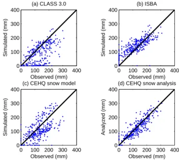
A comparison of the results in Fig. 15 with the CEHQ analysis (Fig. 15d) and with the degree-day model used by the CEHQ provides the first estimates of the analysis’ perfor-mance (Fig. 15c). Because the CEHQ only provides an
anal-0 100 200 300 400 0 100 200 300 400 Observed (mm) Simulated (mm) (b) ISBA 0 100 200 300 400 0 100 200 300 400 Observed (mm) Simulated (mm) (a) CLASS 3.0 0 100 200 300 400 0 100 200 300 400 Observed (mm) Simulated (mm)
(c) CEHQ snow model
0 100 200 300 400 0 100 200 300 400 Observed (mm) Analyzed (mm)
(d) CEHQ snow analysis
Fig. 15. Verification of MESH SWE predictions against snow
sur-vey observations used in the CEHQ analysis.
ysis for select snow survey sites in the Ottawa River basin, the results plotted for CLASS and ISBA are limited to those from the CEHQ-analyzed stations. This seems to improve the results for ISBA (compare Fig. 14b with Fig. 15b), indi-cating that we are eliminating observations which are more difficult to predict.
The improvement between Fig. 15c and Fig. 15d is caused entirely by the data assimilation technique, which updates the SWE and snow depth prognostic variables of the snow model each time a new snow survey observation is obtained. Note that to ensure we are comparing the analysis against indepen-dent observations, we used the analysis value corresponding to 03:00 h before the observation is taken to create Fig. 15d. As previously stated, the CEHQ snow model is forced with precipitation observations, whereas ISBA and CLASS are forced with short-term forecasts. The results indicate that while ISBA shows more bias than the CEHQ snow model and analysis, the variability of the errors obtained with ISBA is similar to the variability of the analysis, and smaller than that of the CEHQ snow model. It thus seems that in using MESH forced by short-term forecasts, we can obtain SWE short-term forecasts that are generally better than the sim-ulated values obtained with a degree-day model forced by observations of precipitation, and almost as good as a snow analysis based on snow survey observations.
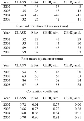
Table 1 presents the bias of each of the four SWE predic-tion techniques for each year, the standard deviapredic-tion and the root mean square of the error made by each SWE predic-tion technique, as well as the correlapredic-tion coefficient between predicted and observed SWE. Except for 2002, ISBA outper-forms CLASS, both in terms of RMS error and bias. When
Table 1. Bias, standard deviation of the error, root mean square
error and correlation coefficient of different SWE predictions for the Ottawa River basin
Bias (mm)
Year CLASS ISBA CEHQ sim. CEHQ anal.
2002 –17 46 –16 –8
2003 –35 26 –48 –12
2004 –63 –12 –49 –11
2005 –32 26 42 11
Standard deviation of the error (mm)
Year CLASS ISBA CEHQ sim. CEHQ anal.
2002 52 27 43 29
2003 53 43 44 30
2004 59 43 48 32
2005 59 37 36 33
Root mean square error (mm)
Year CLASS ISBA CEHQ sim. CEHQ anal.
2002 54 53 45 30
2003 63 50 65 33
2004 86 44 68 34
2005 67 45 55 35
Correlation coefficient
Year CLASS ISBA CEHQ sim. CEHQ anal. 2002 0.72 0.91 0.77 0.90 2003 0.66 0.75 0.72 0.88 2004 0.68 0.85 0.84 0.91 2005 0.70 0.90 0.91 0.91
we compare ISBA (forced by forecasted precipitations) with the CEHQ snow model (forced by observed precipitations), we can see once again that, except for 2002, ISBA outper-forms the CEHQ snow model. In 2002, ISBA snow simula-tions exhibited a large positive bias, which lead to a higher RMS error. Still, in looking at the correlation coefficient for that year, we see that the ISBA short-term SWE forecasts gave marginally better results than the analysis. In fact, look-ing at the correlation coefficient for all years, we can see that ISBA performs as well or better than the CEHQ snow model, and often as well as the CEHQ analysis, even if MESH is not using any precipitation nor any SWE observations. Given these results, we feel that we can use ISBA with some confi-dence to issue ensemble SWE forecasts.
7.3 Verification of an ensemble snow extent forecast We also designed an experiment to illustrate the potential of MESH for ensemble snowpack prediction. Starting from the surface analysis used in the operational version of the re-gional configuration of GEM on 16 March 2003, we forced ISBA with each of the 16 ensemble members of the Cana-dian EPS for one week, resulting in an ensemble forecast of
Fig. 16. NESDIS IMS snow cover analysis for the Great Lakes
region valid for (a) 16 March, 2003 and (b) 23 March 2003.
Fig. 17. Ensemble mean of snow depth, forecast issued on 16
March, valid on 23 March 2003.
the snowpack state for 23 March. As shown by Fig. 16, ac-cording to the NESDIS ISM analysis, the snow line retreated during that week on the U.S. side of the basin as well as in Southern Ontario. However, some snow remained in North-ern Michigan (Area A) and east of Lake Erie (Area B). If we look at the ensemble mean of the 7-day forecast (Fig. 17), we see that the ensemble snow depth mean looks similar to the analysis, except that snow has melted too fast in areas A and B, as well as on the Northern side of Lake Ontario (Area C on Fig. 16). If we examine the individual ensemble mem-bers (Fig. 18), we see that a few memmem-bers have some snow
Fig. 18. Ensemble forecasts of snow depth issued on 16 March, valid on 23 March 2003.
Fig. 19. ISBA snow depth prediction valid on 23 March 2003.
left in Northern Michigan (Area A), indicating there was un-certainty according to the ensemble prediction in this area. However, snow has essentially disappeared for all members in areas B and C.
One way to tell whether the forecast errors for these areas is caused by the atmospheric forecast or by the land-surface system is to run MESH with short-term (06:00 h–18:00 h) forecasts from the GEM model, as was done in the previ-ous section. By running ISBA in this manner from 1 March
2003, we obtained a snow depth prediction different from the ensemble mean (cf. Fig. 19), but which corresponds better to the analysis, especially for areas A and C. ISBA has however melted all snow in Area B.
While we have shown that MESH can be used to obtain ensemble snowpack predictions, a more thorough validation of the ensemble forecast is needed. However, as mentioned before the Canadian EPS has changed considerably in the last two years, and continues to evolve. In particular, starting January 1st, 2006, half of the members of the ensemble sys-tem now use ISBA instead of Force-Restore as a land-surface scheme, so that we need to experiment with this new system. Preliminary results show that members of the EPS which use the GEM model and the land-surface scheme ISBA per-form better at predicting snow water equivalent (Fortin et al. (2006)).
8 Conclusions
To determine the specific requirements for MESH, its differ-ent compondiffer-ents were implemdiffer-ented on the Laurdiffer-entian Great Lakes watershed, situated on the Canada-US border. This experiment showed that MESH can help us better understand
the behaviour of different land-surface models, test different schemes for producing ensemble streamflow forecasts, and provide a means of sharing the data, the models and the re-sults with collaborators and end-users.
8.1 Improving MESH through collaborations
The two main advantages of the MESH modelling system are that it is a community system and that it is part of an opera-tional forecasting system in use at Environment Canada. This not only means that researchers and end-users can use it and modify it freely, but also that MESH should continue to im-prove over the years, benefiting from imim-provements made to the modelling system for research and operation purposes2. In fact, the development of MESH ties directly into a se-ries of existing projects and programs in Canada. Current projects in Canada that plan to use MESH as a modelling platform include the Drought Research Initiative (DRI), the National Agri-Environmental Standards Initiative (NAESI), the International Polar Year (IPY), and the Improved Pro-cesses and Parameterizations for Predictions in cold regions (IP3).
The modelling component of DRI will help researchers to understand and improve the model physics in drought-prone areas, determine the impact of different model physics on the South Saskatchewan River Basin (SSRB), and ultimately improve our ability to make predictions in drought-prone re-gions.
The same basin (SSRB) will be used for modelling within NAESI, with a focus on predicting available water supplies in agriculturally-dominated watersheds. MESH will be as-sessed for its ability to derive products for water assessment, including streamflow and local runoff. The model will also be tested for its ability to estimate near-real time surface state variables such as snow cover and soil moisture using the Canadian Land-data Assimilation System (CaLDAS). In ad-dition, the accuracy of assimilated precipitation products in the region will be quantified using observations, MESH and ground-based radar within the CaPA program. MESH will also be integrated with the Water Use and Analysis Model (WUAM) for assessing water use and availability for irriga-tion planning purposes. The final deliverable relating MESH and NAESI is to identify technologies and products from an operational modelling framework that will provide informa-tion for improved management and planning for agricultural related water practices.
The IP3 project will focus on parameterizing, validating and improving MESH for weather, water and climate sys-tems in cold regions. Scientific hydrologists will be perform-ing studies at a number of basins representperform-ing a variety of typical cold-region hydrological regimes. It is hoped that the
2MESH is not currently available online, but should soon be.
However, the source code of the MEC system on which MESH is based can be downloaded at http://collaboration.cmc.ec.gc.ca/ science/rpn.comm.
studies in these basins will lead to the development of pro-cess algorithms and parameterizations that will be used to test MESH in cold regions.
The IPY project will use MESH to estimate freshwater flux to the Arctic Ocean, help identify knowledge gaps and improve process and parameter representation in the arctic is-lands. Similar to IP3, increased observations of streamflow, snow, water bodies, frozen soil and permafrost mass and en-ergy fluxes at a number of research basins will be used to test MESH algorithms and parameterizations in the high arctic. 8.2 The HEPEX Great Lakes testbed project
Another important project through which we plan to test and improve MESH is the HEPEX Great Lakes testbed project. HEPEX Great Lakes seeks to demonstrate the importance of relatively detailed atmospheric and hydrologic modelling for medium-range atmospheric and hydrologic forecasting on large basins. It will also attempt to assess the added economic value of using ensemble weather predictions instead of climatology for lead times of up to two weeks. The HEPEX Great Lakes testbed initiative aims to help bridge the gap between research and water resources man-agement in ensemble streamflow forecasting by assisting and encouraging researchers and water resources managers in using the same forecasting system, MESH. HEPEX Great Lakes deliverables include ensemble streamflow predictions for individual subwatersheds, joint ensemble forecasts of the Ottawa River flows and Lake Ontario inflows, as well as ensemble snowpack predictions, which could be serviceable to users running their own hydrological models on a smaller scale. More details on the HEPEX Great Lakes testbed project can be found on the HEPEX project website at http://hydis8.eng.uci.edu/hepex/testbeds/GreatLakes.htm.
Edited by: R. Rudari
References
Anderson, E. A.: National Weather Service River Forecast System-Snow Accumulation and Ablation Model. National Oceano-graphic and Atmospheric Administration, Silver Springs, Md., Tech. Memo NWS HYDRO-17, 1973.
B´elair, S., Crevier, L.-P., Mailhot, J., Bilodeau, B., and Delage, Y.: Operational Implementation of the ISBA land surface scheme in the Canadian regional weather forecast model. Part I: Warm sea-son results, J. Hydromet., 4, 352–370, 2003.
B´elair, S., Brown, R., Mailhot, J., Bilodeau, B. and Crevier, L.-P.: Operational Implementation of the ISBA land surface scheme in the Canadian regional weather forecast model. Part II: Cold season results, J. Hydrometeorol., 4, 371–386, 2003.
Benoit, R., Pellerin, P., Kouwen, N., Ritchie, H., Donaldson, N., Joe, P., and Soulis, E.: Toward the use of Coupled Atmospheric and Hydrologic Models at Regional Scale, Mon. Wea. Rev., 128, 1681–1706, 2000.
Cˆot´e, J., Gravel, S., M´ethot, A., Patoine, A., Roch, M., and Stan-iforth, A.: The operational CMC-MRB Global Environmental Multiscale (GEM) model: Part I - Design considerations and for-mulation, Mon. Wea. Rev., 126, 1373–1395, 1998.
Fortin, J.-P., Turcotte, R., Massicotte, S., Moussa, R. and Fitzback, J.: A distributed watershed model compatible with remote sensins and GIS data, Part 1: Description of the model, ASCE J. Hydrol. Eng., 6(2), 91–99, 2001.
Fortin, V., Turcotte, R., Pellerin, P., Seidou, O., and Tapsoba, D.: Taking into account the uncertainty on the state of the snowpack in hydrological forecasts. Poster presented at the 2nd Quantita-tive Precipitation Forecasting and Hydrology Symposium, Boul-der, Colorado, May 4–8, 2006.
Government of Canada and United States Environmental Protection Agency (1995). The Great Lakes: An Environmental Atlas and Resource Book, Third Edition. Available online at http://www. epa.gov/glnpo/atlas/.
Houtekamer, P. L., Mitchell, H. L., Pellerin, G., Buehner, M., Char-ron, M., Spacek, L., and Hansen, B.: Atmospheric data assimila-tion with an ensemble Kalman filter: Results with real observa-tions, Mon. Wea. Rev., 133, 604–620, 2005.
Kouwen, N., Soulis, E. D., Pietroniro, A., Donald, J., and Harring-ton, R. A.: Grouping Response Units for Distributed Hydrologic Modelling, ASCE J. Water Resour. Manage. Planning, 119(3), 289–305, 1993.
Mahfouf, J.-F., Brasnett, B., and Gagnon, S.: A Canadian precipi-tation analysis (CAPA) project. Description and preliminary re-sults, Atmos.-Ocean, 45(1), 1–17, 2007.
Mailhot J., Belair, S., Lefaivre, L., Bilodeau, B., Desgagne, M., Girard, C., Glazer, A., Leduc, A.-M., Methot, A., Patoine, A., Plante, A., Rahill, A., Robinson, T., Talbot, D., Tremblay, A., Vaillancourt, P., and Zadra, A.: The 15-km version of the Cana-dian regional forecast system, Atmos.-Ocean, 44(2), 133–149, 2005.
Matheron, G.: Principles of geostatistics, Economic Geol. 58, 1246–1266, 1963.
Noilhan, J. and Planton, S.: A simple parameterization of land sur-face processes for meteorological models, Mon. Wea. Rev., 117, 536–549, 1989.
Pellerin, G., Lefaivre, L., Houtekamer, P., and Girard, C.: Increas-ing the horizontal resolution of ensemble forecasts at CMC, Non-lin. Processes Geophys., 10, 463–468, 2003,
http://www.nonlin-processes-geophys.net/10/463/2003/.
Pellerin, P., Ritchie, H., Saucier, F. J., Roy, F., Desjardins, S., Valin, M., and Lee, V.: Impact of a Two-Way Coupling be-tween an Atmospheric and an Ocean-Ice Model over the Gulf of St. Lawrence, Mon. Wea. Rev., 132(6), 1379–1398, 2004. Pietroniro, A. and Soulis, E. D.: A Hydrology Modelling
Frame-work for the Mackenzie GEWEX Program, Hydrol. Processes, 17, 673-676, 2003.
Ramsay, B. H.: The interactive multisensor snow and ice mapping system, Hydrological Processes, 12, 1537–1546, 1998.
Shaw, D. A., Martz, L. W. and Pietroniro, A.: A Methodology for Preserving Channel Flow Networks and Connectivity Pat-terns in Large-scale Distributed Hydrological Models, Hydrol. Processes, 19, 149–168, 2005.
Soulis, E. D., Snelgrove, K. R., Kouwen, N., and Seglenieks, F. R.: Towards closing the vertical water balance in Canadian at-mospheric models: coupling of the land surface scheme CLASS with the distributed hydrological model WATFLOOD, Atmos.-Ocean, 38(1), 251–269, 2000.
Soulis, E. D., Kouwen, N., Pietroniro, A., Seglenieks, F. R., Snel-grove, K. R., Pellerin, P., Shaw, D. W. and Martz, L. W.: A frame-work for hydrological modelling in MAGS, in: Prediction in Un-gauged Basins: Approaches for Canada’s Cold Regions, edited by: Spence, C., Pomeroy, J. W. and Pietroniro, A., Canadian Wa-ter Resources Association, 119–138, 2005.
Toth, Z., Lefaivre, L., Brunet, G., Houtekamer, P. L., Zhu, Y., Wobus, R., Pelletier, Y., Verret, R., Wilson, L., Cui, B., Pel-lerin, G., Gordon, B. A., Michaud, D., Olenic, E., Unger, D., and Beauregard, S.: The North American Ensemble Forecast Sys-tem (NAEFS). Proc. of the 18th Conference on Probability and Statistics in the Atmospheric Sciences, American Meteorological Society, Atlanta, January 28–February 2, 2006.
Turcotte, R., Fortin, L.-G., Fortin, V., Fortin, J.-P. and Villeneuve, J.-P.: Operational analysis of the spatial distribution and the tem-poral evolution of the snowpack water equivalent in southern Qu´ebec, Canada, Nordic Hydrology, submitted, 2006.
Valcke, S., Caubel, A., R.,, and Declat, D.: OASIS3 User’s Guide, PRISM Report Series No 2 (5th Ed.), CERFACS, Toulouse, France, 60 pp, 2004.
Verseghy, D. L.: The Canadian Sand Surface Scheme (CLASS): Its history and future, Atmos.-Ocean, 38(1), 1–13, 2000.