Publisher’s version / Version de l'éditeur:
Powder Technology, 83, 1995
READ THESE TERMS AND CONDITIONS CAREFULLY BEFORE USING THIS WEBSITE. https://nrc-publications.canada.ca/eng/copyright
Vous avez des questions? Nous pouvons vous aider. Pour communiquer directement avec un auteur, consultez la première page de la revue dans laquelle son article a été publié afin de trouver ses coordonnées. Si vous n’arrivez pas à les repérer, communiquez avec nous à [email protected].
Questions? Contact the NRC Publications Archive team at
[email protected]. If you wish to email the authors directly, please see the first page of the publication for their contact information.
NRC Publications Archive
Archives des publications du CNRC
This publication could be one of several versions: author’s original, accepted manuscript or the publisher’s version. / La version de cette publication peut être l’une des suivantes : la version prépublication de l’auteur, la version acceptée du manuscrit ou la version de l’éditeur.
Access and use of this website and the material on it are subject to the Terms and Conditions set forth at
A hydrodynamic simulation of mineral flotation. Part I: the numerical
model
Darcovich, Kenneth
https://publications-cnrc.canada.ca/fra/droits
L’accès à ce site Web et l’utilisation de son contenu sont assujettis aux conditions présentées dans le site LISEZ CES CONDITIONS ATTENTIVEMENT AVANT D’UTILISER CE SITE WEB.
NRC Publications Record / Notice d'Archives des publications de CNRC:
https://nrc-publications.canada.ca/eng/view/object/?id=a600a05a-1ae5-42f7-a220-a4c3430dc5e1 https://publications-cnrc.canada.ca/fra/voir/objet/?id=a600a05a-1ae5-42f7-a220-a4c3430dc5e1
E L S E V I E R Powder Technology 83 (1995) 211-224
POWDER
TECHNOLOGY
A hydrodynamic simulation of mineral flotation. Part I: the
numerical m o d e l *
K. Darcovich
Institute for Environmental Research and Technology, National Research Council o f Canada, Ottawa, Ont. KIA OR6, Canada Received 14 February 1994; revised 12 December 1994
Abstract
Mineral flotation is a process whereby particulates containing mineral bearing constituents preferentially adhere to gas bubbles in a liquid medium. This is a way to separate and upgrade ores or other mineral matter. In order to simulate this unit operation hydrodynamically, a three-phase system for the liquid phase and dispersed solids and bubbles must be employed. Additional simulation features are the cell geometry, the boundary conditions, drag terms, variable viscous effects, and the treatment of the adhesion of particles to bubbles. This paper, the first of a series of two, details the formulation of the governing equations, the numerical implementation and shows some results for a two-dimensional, incompressible case. The formulation and implementation are sufficiently general and this simulation was applied to the flotation of coal-oil agglomerates as detailed in Part II of this series.
Keywords: Flotation; Three-phase flow; Turbulence; Finite-volume method; Interphase mass transfer
1. I n t r o d u c t i o n
Mineral flotation is a unit operation where large tanks or cells containing particle-bearing slurries are subjected to turbulent mixing with gaseous bubble streams to provide sufficient contacting between the dispersed phases. Fundamentally, mineral flotation in- volves the collision and subsequent attachment of a particle with a bubble in an aqueous medium. Often, this operation involves selective adhesion of a mineral bearing particle rather than a gangue particle, so in effect the mineral content is recovered in an enriched state. This event is highly influenced by the overall hydrodynamics of all three phases in a flotation cell. In addition to the surface chemical factors which es- sentially influence the particle-bubble attachment, hydro- dynamics simultaneously assist in determining such an interaction, potentially giving rise to a collision, at- tachment and successful flotation.
O f interest in this study are how the prevailing hydrodynamics in this three-phase system produce the sum of interactions which define the efficiency of the unit operation. Since the flow p h e n o m e n a involved can be complex, resolving the hydrodynamic forces would
¢' NRCC No. 37582. Elsevier Science S.A.
SSDI 0 0 3 2 - 5 9 1 0 ( 9 4 ) 0 2 9 5 9 - R
provide a basis for decoupling the surface chemical contribution to the kinetics of mineral flotation.
T h e r e has been considerable research in the past on the role of hydrodynamics in the elementary bubble-particle collision in flotation, as well as to characterize the macroscopic behaviour of a flotation cell. Early work based on the initial model by Sutherland [1] focused on how a particle following a fluid streamline around a bubble in a potential flow regime could contact the bubble. Later research by Flint and Howarth [2], Derjaguin et al. [3], Schulze and Gottschalk [4], Weber [5], W e b e r and Paddock [6] and Dobby and Finch [7] developed hydrodynamic collision models where inertial effects from the particle and flow regimes in an in- termediate range between Stokes and potential flow were considered. Thus, the understanding of how one bubble interacts with one particle had been refined.
The other principal method to model flotation, has been to apply some basic hydrodynamic-related treat- ment to simulate the entire unit operation of a flotation cell. Several papers on this topic have been summarized in a review by Mavros [8]. Typically some mixing pattern was assumed and applied to a residence time distribution for kinetic models scaled up from bubble-particle in- teraction analyses. A comparatively in-depth study by Dobby and Finch for column flotation systems [9,10],
212 K. Darcovich / Powder Technology 83 (1995) 211-224
made use of experimental residence time measurements to model the unit under a modified plug flow regime, without any mechanically introduced turbulence. The particulate concentration was' determined in the axial dimension only via regular differential equations using an axial dispersion coefficient to account for some turbulent action.
The computational fluid dynamics (CFD) approach for the present work was adopted as a means to enable flotation to be modeled in an integrated sense. This work is part of an on-going project on the recovery and beneficiation of waste coal fines by oil agglomeration [11]. Part II of this series [12] describes in detail the surface chemical aspects of the project. The objective of this paper (Part I) is to detail the formulations for simulating the steady-state motion of the liquid, gas and solid phases in a continuous float cell, such that the contacting patterns can be resolved. That is, to provide a mechanistically based model of flotation, the necessary steps of collision and adhesion must be ac- counted for. By determining a three-phase flow field solution, a turbulence based collision model based on local relative velocities and dispersed phase concen- trations can be used to illuminate how the particulate surface properties lead to successful bubble-particle adhesion. Part II in this series will then apply this simulation to flotation recovery data for coal-oil ag- glomerates in order to demonstrate the surface chemical influence on bubble-particle adhesion in flotation. With a resolved flow field, the influence of the particulate surface properties can be decoupled from the hydro- dynamics of the system, which in previous studies, had to be considered simultaneously.
2. M a t h e m a t i c a l model
The general partial differential equations which gov- ern fluid transport were employed in this simulation. Modification of these equations from their basic forms was required to incorporate an interdependent multi- phase system.
2.1. System variables
The system to be simulated in this project required the resolution of twelve different field variables. Since the simulation was modeled as incompressible and in two-dimensions, the field variables were the two di- rectional components of the liquid, gas and solid phase velocities, the pressure, two turbulence parameters, the gas and solid phase volume fractions and the extent of particle adhesion onto the bubbles of the gas phase. The present model allows for the distinct flow paths and local velocities of each of the three phases. The flow field solution produces a two-dimensional velocity
vector field and a scalar field of all other variables. Each phase is treated as a continuum and they share the domain according to the local volume fractions. The dimensions of the interfaces between the liquid and dispersed phases are prescribed by the volume fraction of each dispersed phase subdivided into par- ticles or bubbles of each input diameter. The interfacial area thus determined reflects the multi-phase nature of the model.
2.2. Governing equations
The finite-volume formulation used in this work employed the basic mass and momentum transport equations with the turbulence features worked into them expressed as statistical averages of the random fluctuations. The turbulence in the flows is accounted for by the turbulent variables k and E, from the two- equation model developed by Launder and Spalding [13]. The problem is fully defined with the specification of boundary conditions.
2.2.1. Transport equations
The instantaneous properties of a flow are given by the mass and momentum conservation equations [14]. The variables, u, p and P are respectively velocity, density and pressure. For brevity, the Einsteinian indicial notation is used, subscripts i, j and k referring to the spatial directions.
ap
Mass: ~ + (pu)j.j=0 (1)
Momentum: a(pu)i + [(pu)jul].j = - P i + ~ij j (2)
~t " '
Above, ~-~j is the shear stress tensor given by: 2
7"ij = ].Z(Ui, j "t- Uj, i) -- 3 ~'£Uk. k~ij ( 3 )
Here, /x is the laminar viscosity of the fluid.
2.3. Turbulence model
Via dimensional analysis, two parameters are required to evaluate /z,. The k - E model [15] has proven to be a suitable method to model turbulent flows. The pa- rameters have a physical significance, and transport equations may be obtained for them in a straightforward manner. For high Reynolds number flows, the parameter e is defined as,
P
Here, u; is the mean velocity fluctuation and e defines the dissipation rate of the turbulent kinetic energy.
K. Darcovich / Powder Technology 83 (1995) 211-224
213From dimensional analysis, the relation between the turbulent viscosity/xt and the two turbulence parameters is,
C~,(p)k 2
,u,, = (4)
E
In Eq. (4), C~, is found empirically, and for high Reynolds numbers, has a value of about 0.09. From these expres- sions, equations entirely analogous to Eqs. (1) and (2) can be written [16]. These equations rely on a 'density- weighted ensemble-averaged' (DWEA) form for the field variables. That is, the field terms will be treated with a mean value, but a non-zero time-average for turbulent effects is included.
2.3.1. Turbulent kinetic energy transport equation
The variable k is solved for in the flow domain with its behaviour defined by a transport equation. The DWEA turbulence energy transport equation was de- rived by Watkins [17] by manipulating the momentum equation and making use of the relations between the fluctuating a n d mean flow variables. The form of the equation that is used in this work is,
i)((P)k+((p)t~ik-l(I.~+Izt)k.j )
at ~r k , J
2
= ]J,t(/,~i(/,~i, j "~-/,~j, i)). i - ~ (/~j[~/,t/~i, i"[- ( p ) k ] ) , j - (p)E
(5)
The notations (p) and fi~ refer to, respectively, an averaged value and a density-weighted ensemble-av- eraged value. In Eq. (5), irk is an empirical constant of value 1.0.2.3.2. Turbulence energy dissipation rate equation
The ensemble-averaged energy dissipation equa- tion is given below, in terms of DWEA variables, as this form [17,18] is considered the most correct, of the available relevant formulations. It is written
as, i ) ( ( p ) , ) _b ( (p)/~j, _ L (1~ .k_/./,t),..i ) bt o-, J e { c [ t x ( t ~ ( t i , . i + d j )) k 1 t i , i , j
~ (/~j(l"/'t/'~i, i "~-
(P)k)),i]-C2(p)e]
+C3(p)a~j.j (6)The model constants, cr,, C1, Cz and C3 are given in Table 1.
Table 1
Turbulence model constants
Constant C~, CI (?2 K E ~r k o-, Ca Value 0.09 1.44 1.92 0.4187 9.793 1.0 ~ 1.0
(C2 - C l ) C ~ 5
Table 2
Interphase drag terms for the momentum equations Phases Drag term
9~G/.t,L .
liquid-gas
FLGi= T
['UGi--UlA)liquid-solid FLsi =B(uu--Usi)
2.4. Three-phase model 2.4.1. Gas-phase equations
Continuity: (aopouoi).i=O (7)
Momentum: aG(pGUGiU~i-- p.GeffUGi.j).j
= -- otGP, i + otGPGgi +FGLi + ao3ri(pc, UG, P-ceff)
(8)
Above, aG is the gas-phase volume fraction, and the term FGL is the interphase drag term for the gas phase in relation to the liquid phase [19,20]. The terms indicated by 9-~(pc, uG,/zG~fr) arise from the curvature of the coordinate system selected. For this work, a Cartesian system was used, and these terms drop out. The interphase drag terms are summarized in Table 2. The effective viscosity term, /zceer is the sum of laminar and turbulent contributions to the viscosity. In this simulation,/zG, is not considered as the turbulence is restricted to the main transporting phase, which is the liquid.Based on assumptions made by Lai and Salcudean [19], the gas-phase momentum equations may be sim- plified. The gas phase is assumed to be dispersed in the liquid phase. Further, in typical mineral flotation applications, the presence of chemical frothers and conditioners causes the bubbles to act as rigid spheres [5]. The gas bubbles are also modeled as incompressible which is a simplifying assumption; in this way, a constant system volume may be obtained. Further, inherent instabilities such as oscillations at the free surface of the vessel are neglected. The bubbles are treated as having a constant given diameter which therefore does not allow for coalescence. Naturally, bubble coalescence is a very real phenomena, but incorporating it into this model would introduce a great deal of complexity to a system which is a first step in flotation modeling by the solution of field equations. Coalescence would serve to increase the mean bubble size and reduce the number
214 K. Darcovich / Powder Technology 83 (1995) 211-224
density of bubbles thereby contributing to a lesser flotation recovery.
Despite these shortcomings, the simulation can dem- onstrate the basic physical behaviour of the system. In any case, simplifications of the physical geometry of the flotation unit used in the simulation are made, such that an overly complex and completely physically correct treatment of the gas-phase behaviour would be superfluous.
If the action of the liquid phase is assumed to be primarily responsible for the gas-phase transport, then only the pressure, drag and buoyancy terms are retained. In this way, the gas velocities may be explicitly determined from the gas velocity term in the drag expression. The resulting momentum equation becomes, 0 = --aoP~+aGpGgi+FGL~+aGSr~(pG, UG, /ZG.,,) (9)
2.4.2. Liquid-phase equations
Continuity: (aLPLUL~). i = 0 (10) Momentum: aL(pL ULjUL~ -- /ZL~ffUL~. j). i
= --aLP'.~+FLGI+FLsi+aLSrI(PL, UL, /ZLaf) (11)
Above, aL is the liquid-phase volume fraction. In Eq. (11), the term aLPLg~ is omitted since the equation makes use of a corrected pressure P', where,
P ~ i - - P , i + pl_gi
Hence, it can be seen that using P' instead of P takes care of this term. The interphase friction terms are the same ones as given in Table 2. It should be noted that in general, when a phase 1 interacts with a phase 2 in a j-direction, it can be said,
F 1 2 j = - F 2 1 j
Hence, with respect to equations for other phases, the signs are reversed on the interphase drag terms when inserted into the liquid-momentum equation.
2.4.3. Solid-phase equations
Continuity: (aspsUs,), ~= 0 (12) Momentum: as(psUsjUs~).j
= -otsPi+asPsg~+FsLi+asSrsi(Ps, Us) (13)
Above, as is the solid-phase volume fraction. F o r the solid phase, the viscous terms will be of a negligible magnitude in comparison with the inertial terms, and are thus dropped from Eq. (13).
2.4. 4. Interphase drag
Based on results from Soo [21] and Lai and Salcudean [19], the liquid-gas and liquid-solid interphase drag terms are given in Table 2. Also in Table 2 we have the coefficient B for the liquid-solid interphase drag coefficient. This term is based on derivations by Ergun
[22], Wen and Yu [23] and Lyczkowski and Wang [20]. We use s ¢ and ~s to refer to normalized (gas phase excluded) liquid and solid volume fractions. This ap- proximation is made as it is assumed that the liquid phase is responsible for transporting the dispersed phases, and that gas-solid and solid-solid interactions are neglected. O~ L O~ L --1- O~ S Also, a s ~ s - - - -Ot~L + Ot~ S
As shown in [20], two cases are considered for B. We have,
PLluL,--UsII s
for ~:s>0.2 (14) B = 150 ~ + 1.75 2rpIn dense slurries, the flow field disturbances around spheres begin to overlap and hence a separate expression is needed for such a case. For more dilute liquid-solid systems, a different regime exists and is modeled [20,23] a s ,
B=0.75CD
U26 slu '-u 'I
for ~s<0.2 (15)2rp
Rowe [24] related the drag coefficient to the Reynolds number by,
t 24
CD = Re~ (1 + 0.15Re~ °687) for Res < 1000
0.44 for Res >~ 1000 where,
R e s 2~pL(UL-- US)rp
I~L
2.4.5. Multi-phase mass balance
Throughout the flow domain, a check must be made on the sum of the volume fractions of the various phases. At all locations, the following condition must be satisfied,
E a M = 1 (16)
M
Continuity of phases
In this simulation, there are three phases considered, water, bubbles of varying particle loading, and particles. Each phase is subject to a momentum balance which is employed for the calculation of its respective velocities, which in turn must be used to determine local volume fractions to ensure proper continuity for each phase,
K. Darcovich / Powder Technology 83 (1995) 211-224 215
and taken all together, to conserve an overall, multi- phase mass balance.
Liquid phase
As described by Lai [16], the main transport phase velocities are determined by solution of the momentum equation, and then the conservation of mass is ensured by coupling the velocity determination with a pressure correction, which diminishes with convergence. The volume fraction for the liquid phase is not explicitly calculated, rather it is simply calculated as the remaining volume fraction, once gas and solid phase volume fractions have been calculated. That is, the liquid volume fraction, aL is calculated as,
aL = 1 - a c - as (17)
If at any point in the numerical computation of the phase volume fractions, the local sum of them exceeds unity, then they are all simultaneously normalized fol- lowing, O/i ai = 3 (18) ~ a j j - 1
Gas phase
A local flux balance at all nodes in the grid is employed to determine the gas phase volume fraction at all points in the flow domain. This is based on an upwind scheme presented by Spalding [25].
We can express the flux Gi, for the ith phase, as
G=p./lul,
where A is the area of the face throughwhich this flux takes place. A local flux balance for any phase can be written as,
E aiGi = ~otiGi+R i
(19)CUT IN
The term R~ refers to a mass generation or consumption in a finite-volume cell. The adhesion of particles to bubbles represents a mass transfer from the solid to gas phase. The derivation of this term is discussed in section 2.4.7. Any outgoing flux from a cell will represent the volume fraction oqtp J in that cell. The incoming fluxes will contain the volume fractions in the respective neighbouring cells. We can rewrite Eq. (19) in view of the upwind differencing scheme as,
a~tP I ~ Gi =
ZoqG,+R~
(20)OUT IN
Now, we have a finite volume expression for o~ijpl , which is the unknown volume fraction at the point P, or cell where this flux balance is applied.
' ~ a i G i -I-- R i IN
°t'IPl- ~ Gi
C U T
Substituting the above result into Eq. (16) gives, ~ a G G G + R G ~ a L G L IN IN + - - + a s = l (21)
E c o
EeL
OUT OUT Rearranging gives,~ GL'(~aGG~+Rc)+ ~ Go'~_~CtLGL
OUT OUT INNow, substituting
(F.IN~aGG+RG)/aGtp I
for ~ouTGc on the right hand side of the above expression, then rearranging gives,(22)
Eq. (22) may be used in the finite volume scheme for solving the gas phase volume fraction, in an iterative fashion, using current values of aL and as to update aGtPl- Upon inspection, it may be seen that Eq. (22) is inherently stable, as it has been constructed to calculate values of aG~Pl which are between 0 and 1.
Solid phase
In a fashion analogous to the previous development for the gas phase, the mass balance for the solid phase was derived.
2.4.6. Turbulent collision model
Successful mineral flotation depends on having suit- able hydrodynamic conditions, or mixing to bring the bubbles and particles into contact with one another, as well as the necessary particulate surface properties to create a lasting adhesion between these particles and bubbles.
With a statistical approach to the collection of par- ticles by bubbles, the micro-kinetics of a flotation system may be expressed. This must be done in view of the prevailing hydrodynamics of the system [26], which can be either laminar or turbulent.
Based on Abrahamson's model [27] for parti- cle-particle collisions in a turbulent fluid, Bischofberger and Schubert [28] derived the following expression for the number of collisions per unit volume per unit time ZpB, in a turbulent flotation system.
216 K. Darcovich / Powder Technology 83 (1995) 211-224
2 2 0.5
ZpB = r,,npnBdea(VpB + g~B) (23)
Here, np and nB are respectively the number concen- tration of particles and bubbles. The term dpB is defined
as,
dpB =rp + rB
The terms Vp and vB are given by,
( E4/9 • d7/9~ [ Ap~ 2/3
vi=0"4~ ~ ]kP--LLJ
Above, Ap= IPi-PLI, and VL is the kinematic viscosity of the liquid phase.
The term r, represents the adhesional probability part of the collision expression. The mechanistic basis of r~ is related to the surface properties of the solid particles and is discussed in Part II of this series [12]. There are a number of limitations which apply to the use of Eq. (23).
This equation was derived from the Smoluchowski equation which predicted the collision rate of two particles under shear flow conditions. The equation is used here only insofar as it provides a basic trend for the collision rate occurring at the each node in the cell. It does not explicitly account for the various physico- chemical processes associated with the collisions such as film-thinning and surface deformation and bounce. The turbulence mixing length l, of the system is defined as, l = 0.025D~. With a 20 cm slurry inlet we have l = 0.005 m, and the bubble diameter is 0.002 m, thereby satisfying the requirement that l > d B for Eq. (23) to be valid. The Bischofberger and Schubert model was selected for this simulation since it can be conveniently applied to a population of particles and bubbles, making direct use of the simulation variables which have been calculated throughout the domain. The flotation col- lision model is applied to the simulation in a fashion analogous to how a drop collision and coalescence model was used for studying liquid sprays [29,30]. In the numerical simulation, the dispersed phases were modeled with their average diameters, so the collision rates from Eq. (23) were used directly. Naturally, it is a simplification to use mean diameters rather than to perform the simulation accounting for the bubble and agglomerate size distributions, but for the purposes of demonstrating the influence of the agglomerate surface properties under prevailing hydrodynamics on observed flotation trends, the present treatment is sufficient. Eq. (23) was found to give plausible results and equally importantly, provided a means to decouple the colli- sional and attachment probabilities involved in flotation. An improved or more sophisticated collision model could be very easily substituted into this simulation, and the resulting functional relationships could be resolved in the same manner as done in this work.
2.4. 7. Interphase mass transfer
The conservation of the mass of a phase is governed by the transport Eq. (24). For this work, it is written in terms of the solid phase, as this is used as the reference phase where material is lost through mass transfer to the gas phase. Below fos is the density fraction of the species in the particulate phase which is participating in the mass transfer [31]. By definition, fps = 1 at the start of any iteration, as the entire par- ticulate phase is considered to be coal--oil agglomerates which are involved in the mass transfer.
- - + (f~suj +Jsj).j
=Rs
(24)at
Above, Jsj is the diffusion flux vector for the solid phase, and Rs is the rate of consumption of the solid phase, in units of kg/s. The term Jsj refers to molecular diffusion, and can be neglected for this system which models large dispersed bodies. Since a steady-state system is being simulated, the time derivative term may also be dropped. Thus Eq. (24) simplifies to,
Rs =fpsuj.~ (25)
The rate term Rs is calculated using the rate of collision term zpB from Eq. (23), which gives a value in units of [collisions s -1 m-3]. Thus,
Rs = r~( NemMAx -- Nem)ZKB VCELL mS (26) There are a number of additional factors in the above expression for Rs. The term,
(Np~MA×-Np~)
expresses the fraction of the bubble surface which is still available to contact a particle. VCELL is the volume of the local cell where this collision rate is applied, and ms is the mass of one solid particle.
Solution of Eq. (25) will produce an array of updated solid phase density fractions f~s, with values between 0 and 1, which represents the fraction of the solid phase remaining after some of it has transferred into the gas phase under the prevailing transport conditions. We set,
R, =fk~
where Ri is the mass generation or consumption term for the ith phase, used in the equations in section 2.4.5 which determine the local volume fractions of the dispersed phases accounting for the transport conditions with simultaneous mass transfer.
Effective mass transfer
The problem being modeled in this work involves transfer of mass from the solid phase to the gas phase. This requires that the effective bubble diameter must increase as mass is transferred. An average bubble size can be computed for each cell in the flow field. To
K. Darcovich / Powder Technology 83 (1995) 211-224 217
do this, we employ the method of Spalding [25] known as the shadow solution.
The shadow volume fraction &c, is the volume fraction the gas phase would have possessed, at each node, if the interphase mass transfer had not taken place. That is, Eq. (19) is employed without the Ri term. However, since these equations represent a continuum where the outgoing fluxes must balance those coming in, Eq. (22) is modified to the form below for determining the shadow volume fraction.
,o P, ( ooo)
(27)
The difference between a o and &c can be attributed to diameter growth via mass transfer. Thus,
d B [ \ 113
Above, ds0 is the diameter of the bubble in the particular cell at the start of the iteration. Further, it can be deduced that,
Vo - Voo
MVp m (29)
Vs
since the gain in gas phase volume is at the expense of the solid phase. The term V~ refers to the volume of one body (bubble or particle) from either the gas or solid phase.
Finally, as will be discussed in the next section, the extent of solid adhesion to bubbles was constrained. Thus, it was assumed that the gas-phase solid loading and corresponding density increase were small enough to allow the simplified gas phase transport equation (Eq. 9) to still apply.
2.4.8. Drag on a loaded bubble Bubble loading
This simulation has incorporated a modified drag on a bubble which has particles adhering to it. Two con- straints were implemented to control the level of par- ticles adhering to a single bubble. The maximum bubble loading is calculated by assuming that circular projec- tions of the areas of the particles may occupy the surface of the bubble. The particles are modeled to pack in a two-dimensional hexagonal lattice, thereby covering a maximum of 90.7% of the bubble's geo- metrical area. The maximum number of particles per bubble, NpmM,,×, is thus,
NemM,,X = 0-907(r4~2B) (30)
A second constraint arises from considering the rel- ative fluxes of the gas and particulate phases in the float cell. Numerical instability could arise if the bubbles became too heavily loaded and gave outlet particulate fluxes greater than their inlet fluxes. Assuming all the inlet gas exits in the product stream (not via the liquid exit) then the maximum number of particles per bubble becomes,
gs PG Vo
N~/BM.x = - - ( 3 1 )
gopsVs
Above gi refers to the flux of the ith phase, and V~ refers to the volume of one dispersed body. In practice, if a mass-flux instability arose, NemM^x was replaced by N~,mM^x in the algorithm.
Particle patches
Particles are modeled to form concentric hexagons on the back side of moving bubbles as shown in Fig. 1. These hexagons are denoted as levels, and the total number of particles at each level, n is,
N I = I n
N, = 1 + ~ ] 6 q - 1) (32) j - - 2
Particle patch drag model
The particle patch was then applied to a model developed by Pendse et al. [32], which was for drag force calculations of spherical collectors with deposited particles in various configurations. For cases with several particles attached, the hydrodynamic interaction among the attached particles must be considered.
For our case, we make the assumption that loaded bubbles transported by fast-moving water will orient
N : N i n t e r a c t i o n s ... N : N - 1 i n t e r a c t i o n s Fig. 1. S c h e m a t i c p a r t i c l e p a t c h .
2 1 8 K. Darcovich / Powder Technology 83 (1995) 211-224
themselves with the particle patch at the rear of the bubble, in line with the velocity vector of the bubble. The drag effects are a function of the position of the particle relative to the bubble's line of motion, as well as the product of all the interaction terms from all the attached particles.
Pendse et al. [32] give the following expression for a multi-particle interaction which augments the drag force.
AFD.Mj=AFo.o'f(PM,.,, PM2.,, PM2.2, ...PMN.j)
(33)Above, AFD.~ j represents the increment of the jth particle from the Mth level on the drag of a bubble carrying such a number of particles. This increment is normalized with respect to the drag of an unloaded bubble. The function f(PM,, a, PM2,,, PM2. 2, ".PM,~.i) rep- resents the interaction of all attached particles with each other. Thus, the overall change in drag for a loaded bubble of N levels, with j particles at this level, AFD[N:j], will be,
N L
~FD[N..jl=Fo.,, + ~ ~ AFo.~,
(34) M = 2 i ~ l L = 1 6 ( M - 1) forM < N
where,tJ
forM = N
The interaction term for only two particles was given in a derivation by Happel and Brenner [33]. The complete derivation of the expressions used to arrive at this loaded bubble drag modifier is given in [34].
As an example, for a bubble of 2.0 mm diameter and a particle of 60/zm diameter, the calculated drag coefficients are illustrated in Fig. 2. These calculations agree with the basic results of Pendse et al. [32] which they only calculated for cases with one and two attached particles.
2.4.9. Viscosity effects
The presence of up to three phases in variable concentration throughout the flow domain necessitates a means for specifying a basic laminar viscosity in each
2 . 0 m m B u b b l e , 6 0 / ~ m P a r t i c l e s 1.010 1 . 0 0 8
i
"G 1.00e e c ¢'~ 1.004 CIt m a 1.002 1.00@ ~ ' ' 2 4 e 8 A t t a c h e d P a r t i c l e s Fig. 2. D r a g f o r c e c o e f f i c i e n t s vs. b u b b l e l o a d i n g . 10cell. The viscosity of a slurry is known to increase with solids concentration. The presence of air tends to give a much reduced viscosity, along the lines of a weighted average of the slurry and air viscosities. Since the viscosity of air is about three orders of magnitude below that of water, its effect is neglected [35]. That is,
/ ' / " T O T A L = (1 - aO)/XSLURRV
A model was incorporated into the simulation to account for variations in the laminar viscosity arising from local conditions. The two effects considered were those of particle size and particle concentration. Data from Borghesani [36] was fitted with a multivariate linear response surface. The response function was
reduced
(or normalized) viscosity, which is the viscosityof the slurry, divided by the viscosity of the pure suspending liquid. Hence, this provides a local coef- ficient, k,,, for the laminar liquid viscosity which is used in the program.
The analysis of the residuals showed an average error of about 8% over the entire range of the model, which extended from 0 to 40 v/o solids concentrations and particle diameters from 1 to 450/zm. A model of this nature was considered adequate to convey any trends associated with the rheological properties of the 3- phase system.
3. Numerical i m p l e m e n t a t i o n
The solution of the discretized differential equations is done via a hybrid of central and upwind differencing in the spatial dimensions, thereby permitting accurate computation over an extended range of Reynolds and Peclet numbers. Each finite volume equation is solved sequentially, in an iterative manner. All of the previous equations which have been expressed as transport equa- tions have assumed a similar format. In fact, any of the transport variables may be represented by a gen- eralized transport variable, ~b. q5 can be interpreted as either a time-average or a density-weighted average. In any case, the form of the equations are all identical. The different averages need not be indicated, as tur- bulence parameters along with the mean flow variables account for the entire flow field description.
In our general form, we have,
a(p4,) + (pu, 4,- F,4,. ,). ,= S , (35)
8t
where F6 and $6 are coefficients respectively known as the effective exchange coefficient and volumetric source rate of the variable .~b.
The computer code developed to implement this finite volume formulation is quite modular in structure, allowing simple specifications to dictate steady or un- steady, laminar or turbulent, compressible or incom-
K. Darcovich / Powder Technology 83 (1995) 211-224 219
pressible, reacting or stable states as well as heat and mass transfer conditions. Grids defining the flow domain may be prescribed in either Cartesian or cylindrical coordinates.
The formulations given above, as well as the numerical devices detailed below, were incorporated into a com- puter code known as MO-PrIASE (multiple, dispersed phases), which was based on previous "I~MA and "rOR- COM codes [16].
3.1. The grid system
The flow domain is divided into control volumes, or for this two-dimensional case, control regions, defined by the coordinate-based grid lines. Fig. 3 illustrates this finite volume grid system. Based on the method of Gosman and Ideriah [37], a staggered grid is used to enhance numerical stability. Scalar qualities are determined at the grid points, and the nodes for the velocities (or vector quantities in general) are displaced in their respective directions to the mid-point of the scalar nodes along the grid lines. Scalar control regions are centered about the point P as indicated in Fig. 3, while the momentum control regions are centered about the points U and V for the respective velocity direction. This particular grid arrangement is well suited for imposing accurate boundary conditions since the mid- point locations for vector variables coincide with those of the normal velocity components, and thus prescribed boundary values and/or fluxes need not be modified.
3.2. Discretization procedure
The differential equations which govern the physics of the flow are integrated over the volume of the flow domain. The entire domain is partitioned into cells delimited by the grid, and the unknown quantities are taken to be constant within each cell, with this mean value assigned to the node point.
P,V grid line U grid line ~ / / U c e l l boundary - i ! i
---ill
....
i
i i : c e . b o u n . . r y P , V c e l l boundary c o n t r o l v o l u m e f o r n o d em
P,U c e l l boundary grid line P,U c e l l boundary V cell boundary rid line V cell boundary Fig. 3. T h e f i n i t e - v o l u m e c o n t r o l r e g i o n for a t w o - d i m e n s i o n a l C a r t e - s i a n system.The general transport equation (Eq. (35)), can be written for the generalized variable, ~b, over one cell volume, Vc, with a time step of &. We can thus write,
d-- f (P4') dV+ f (Ou'4'-r*4"3ni dA= f S*
(36)Vc A c Vc
Above, nl is the unit outward normal from the control surface, Ac. The upwind differencing technique is then applied to this integral form of the transport equation to produce a system of linear equations for the field variables at each node in the domain. The details of such procedures are given explicitly in [16].
3.3. Equation solution algorithm
Beginning with the initial values for all the field variables, the governing equations are solved in sequence until the convergence criteria are satisfied. These are referred to as the outer iterations.
Each linear equation, which is formulated over the domain for each variable, is solved by an inner iteration, an efficient scheme for treating a large matrix.
3.3.1. Numerical solution procedure
The matrix which is assembled for each field variable equation is solved by a block iteration technique. This procedure sweeps across planes defined by coordinate index. A tri-diagonal matrix form is assembled locally as in the Gauss-Seidel method. This matrix can be solved implicitly. Details are given in [16]. The plane is solved grid line by grid line, and is repeated in alternating directions towards convergence. Since this is the inner iteration, full convergence is not required, as coupled variables are being simultaneously modified. The outer iterations ensure full final convergence, so usually no more than three inner sweeps are performed for each variable.
3.3.2. Execution sequence
As seen, the governing finite difference equations are coupled and non-linear, thereby requiring an it- erative method of solution. In each outer iteration, the equations are individually solved with inner iterations in a sequential fashion, adjusting each variable by its own equation, while holding others constant. The steps comprising the numerical algorithm are itemized below. (i) The fields of all variables were initialized either by guess or calculation.
(ii) The liquid phase momentum equation was solved. (iii) The pressure equation was solved, and pressure corrections (to ensure mass balance) were applied to liquid velocity field.
(iv) The turbulence parameters were determined. (v) Gas-phase momentum equation was solved, and gas volume fractions were calculated.
2 2 0 K. Darcovich / Powder Technology 83 (1995) 211-224
(vi) Solid-phase m o m e n t u m equation was solved, and solid volume fractions and 'shadow' solid volume fraction were calculated.
(vii) The extent of solids 'conversion' was calculated and used to update the gas and solid volume fractions and the gas phase solids loading and net diameter.
(viii) Steps 2 through 7 were repeated until the convergence criteria were satisfied.
3.3.3. Convergence criteria
T h e residual sources of each finite volume equation for each variable were compared to a reference tolerance to assess the convergence of each equation. This ref- erence tolerance R,, REF, is selected as the inlet flux of the d e p e n d e n t variable ¢. This convergence criterion indicates how well the current values of ¢ solve the equation in question, rather than how much the values of ~b have changed over successive iterations.
Referring to Eq. 35, which is the generalized finite volume equation, the local residual for the ¢ equation for the ith iteration is defined as,
0 ( p ( ~ ) + (pUi (~ -- F~ b (~, i),i -- S~b ( 3 7 )
R , = at
It can be seen that when the solution is obtained, R , goes to zero. Convergence is considered satisfactory if the sum of the normalized absolute residuals has fallen below a specified value A, in this case selected as 10-1. That is for each ¢ equation,
E EIR,l,.Jll < XR,, ~ (38)
i j
3.4. Boundary conditions a n d simulation inputs
For the flotation simulation the boundary conditions are shown in Fig. 4. The cell is modeled after a commercial cell made by Minpro of Mississauga, Canada and handles a solids throughput of 4.32 tonnes/day and an air rate of 1.5 m3/min. Its dimensions are given in Table 3. The top face of the float cell is considered flat and open to the atmosphere. A zero reduced pressure is imposed here along with the condition that the gas phase may exit in the vertical direction, while UL and Us were set to zero.
Turbulence conditions at inlets were modeled after equations given in [16]. Concretely,
I = 0.005 l = 0.025Di kl.5
k = I u 2 e = l
Above, I is the turbulence intensity, and l is the tur- bulence mixing length, given in terms of the inlet diameter Di.
t
Ovj= 0.0 uL = 0 . 0 , u~ = 0.0, Ou~= 0.0 0y 0x U~ , vj = 0.0 o n a l l w a l l s v~ = 0 . 0 5 v s = 0.0.5 a s = 0.10t
= u G = 0 . 0 5 v c% = 0 . 5 0 Fig. 4. B o u n d a r y c o n d i t i o n s f o r t h e M D - P H A S E f l o t a t i o n s i m u l a t i o n . T a b l e 3 F l o a t cell d i m e n s i o n s P a r a m e t e r Size W i d t h 1.42 m H e i g h t 1.6 m S p a r g e r w i d t h 5 2 . 7 c m S l u r r y i n l e t d i a m e t e r 2 0 c m W e i r d r o p 5 - 1 5 c m T a b l e 4 P h y s i c a l p r o p e r t i e s o f t h e t h r e e p h a s e s P h a s e D e n s i t y V i s c o s i t y D i a m e t e r L i q u i d 997.1 8.94 × 10 - 4 N / A a G a s 1.2 1.42× 10 -6 2.5 m m Solid 1200.0 N / A ~ 2 0 - 6 0 /~m N / A n o t a p p l i c a b l e .There are some additional boundary treatments which are included in the formulation to produce more stable numerical behaviour. These are discussed by Lai and Salcudean [19].
The three phases in this simulation were input the physical properties listed in Table 4. The units are based in the mks system.
The grid used for the simulation is shown in Fig. 5. The regions of high swirl or where streams mix have more grid lines to enhance the resolution. Grid sensitivity was not investigated in this work. The inherent error and limitations of this simulation (ie, simulation in 2D rather than 3D, with simplified geometry) render the results useful in the sense of how they illuminate the simultaneous interplay of the various flotation mech- anisms. The present simulation would need to be run in three dimensions for actual engineering design work.
K. Darcovich / Powder Technology 83 (1995) 211-224 221
II
II
Fig. 5. Finite volume grid used for flotation cell.
I:::::::::::1
~ - ~ ' ~ - - ~ "~ :~ II
• r p t ~ t / ¢ t / t ! I / I [
tit ~ t y ~ / l , ' / ! ! tlJ
e ~
Fig. 6. Three-phase flotation velocity and pressure fields. (dp= 43.6
p,m and r~,=0.20.)
4. Results
A data set for the study of the flotation parameters was constructed by running the three-phase simulation for a combination of particle diameters and values for the attachment efficiency, r,, which was introduced in Eq. (26). This data set was then used to deduce a
relation between the properties of the floated material and its recovery. The surface chemical aspect of this project is detailed in Part II of this paper.
Run-time control was achieved by running all three phases at once, but with the frequency of iteration for the dispersed phases reduced until a stable basic flow field pattern based on liquid transport was established. The frequency of iteration for the dispersed phases was gradually increased until a ratio of 1:1 was stable, and convergence could be achieved.
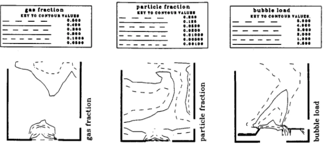
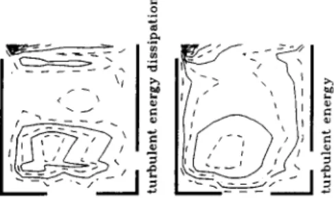
Figs. 6-8 show a full three-phase flotation flow field simulation result. This case had dp=43.6 /~m corre- sponding to an coal-oil agglomerate made with 2 wt.% oil and the attachment efficiency, ra = 0.20. The pressure field shown in Fig. 6 shows the dynamic pressure.
For the example illustrated in these figures, the flux of solids accompanying the gas phase from the top exit was 0.447 kg/s, giving a flotation recovery for this case of 37.2%.
For the other cases run, the graphical output is very similar. The same basic trends are followed. What can be noticed is slight streamline differences for heavier particles. Two cases are shown in Figs. 9 and 10. Another feature evident in Figs. 9 and 10 is that for the 60/.~m case, the streamlines travel at the top of the cell in the y-direction as they exit over the weir. Their greater settling tendency does not enable the flux in this case to transport them up over the weir as with the 20/~m particles. A stronger circulation is established in the top half of the cell to create a current of sufficient flux to carry the unfloated solids out over the weir.
Additionally, Figs. 11 and 12 show streamlines cal- culated for bubble diameters of 2.5 and 1.0 mm re- spectively. The particle diameter in this case is 60/~m. The greater buoyancy force on the larger bubbles renders them less subject to the trajectory deviations brought about by the slurry motion.
g a s f r a c t i o n KeY TO CONTOUR VALUe8
0 . 6 0 0 0 . 4 0 0 0 . 8 0 0 O.JO0 0 , 1 0 0 0 0 . 0 0 0 0 p a r t i c l e f r a c t i o n E l Y ?0 CONTOUR VALUBI 0 , 8 0 0 0 , 1 | 0 o , o s o o o , o 8 0 o O . O l O 0 0 0 . 0 0 0 0 0 o , o e t o o b u b b l e l o a d
ICgY TO CONTOUR VALUES, 0 , 0 0 0 4 , 0 0 0 0 , 0 0 0 0 . 0 0 0 1 , o o o o . s e o Q I \ \ \ J / /
Fig. 7. Three-phase flotation concentration and mass transfer contours. (dp=43.6 ~m and ra=0.20.)
_o
e~ ,.Q
222 K. Darcovich / Powder Technology 83 (1995) 211-224
Fig. 8. T h r e e - p h a s e flotation turbulence contours. (dp= 43.6 ~ m and ro = 0.20.)
Fig. 11. Bubble streamline, d B = 2 . 5 m m .
Fig. 9. Particle streamline, dp=20 ixm.
Fig. 10. Particle streamline, dp=60 lzm.
4.1. Integrated flotation model
The CFD work carried out as part of this project enabled an integrated study of mineral recovery by flotation to be achieved. That is, the output from the unit operation was determined as a sum of all local mass transfer occurring throughout the domain. In this way, the effects which were of a specifically hydro- dynamic nature, such as dispersed phase diameters and densities, the prevailing flow patterns and local tur- bulence accounted for the collisions leading to possible
Fig. 12. Bubble streamline, dB= 1.0 mm.
subsequent mineral collection. Thus, this provided a means to decouple surface chemical effects which were responsible for the adhesion of the particles to the bubbles once a collision had taken place. This is fully discussed in Part II of this paper.
5. Conclusions
A two-dimensional finite volume code for three-phase flow was formulated and implemented to simulate the process of mineral flotation. This model incorporated a turbulent bubble-particle collision model giving rise to interphase mass transfer which defined the flotation process recovery. These effects were successfully coupled with the mass balance equations for each phase. Also included were three-phase rheological effects and a modified drag coefficient for the gas phase when small solid particles adhere to bubble surfaces.
The novel use of a CFD flotation model provided an integrated simulation, allowing recovery predictions on fundamental material properties, and using a micro- flotation collision model in a macroscopic hydrodynamic
K. Darcovich / Powder Technology 83 (1995) 211-224 223 context where all local variables are prescribed. This
ensured soundness of results and an adaptability to various behaviour regimes. The present simulation has been shown to be suitable for making a parametric study of flotation. Part II of this series makes use of resolved hydrodynamics to illuminate attachment phe- nomena for coal-oil agglomerate flotation.
The flow model itself is in a generalized form, so the basic framework is in place to convert to three dimensions. In three dimensions, the full effects of cell geometries come into resolution, and as such, the cell configuration and the turbulence parameters would be highly useful for actual engineering design work.
S ~ t ui l) B l)p
Vc
V ~
Vo
V ~Vs
ZpBSubscripts
volumetric source rate time
velocity
bubble turbulent collision velocity particle turbulent collision velocity finite difference cell volume volume of local cell
volume of one bubble
volume of one bubble at start of iteration volume of one particle
collisions per unit volume per unit time
6. List of symbols A B
Co
C, C1, C2, C3 dB dBo dp deB D i E 3ri Gi IJj~
k k , 1 m s ni nB np Npm P P rB rp ra R t Ri R,b R,[,, Jl R~b, REF Re Resarea of cell face for flux coefficient for liquid-solid drag drag coefficient
k - E model constant k--E model constants bubble diameter
bubble diameter at start of iteration particle diameter
rp+ra
inlet diameter
turbulence model wall velocity constant dispersed phase-liquid interphase drag term curvature related source terms
flux of ith phase turbulence intensity
diffusion flux vector for Jth phase turbulence kinetic energy
laminar slurry viscosity coefficient turbulence length scale
mass of one solid particle unit outward normal
number concentration of bubbles number concentration of particles bubble loading, particles per bubble maximum bubble loading under mass-flux constraint
pressure
finite-volume node point bubble radius
particle radius attachment efficiency rate of flotation
mass generation or consumption of ith phase
residual for ~b equation local nodal residual for 4) reference residual for 4' equation Reynolds number
particle Reynolds number
G , L , S i , j , k
[p]
tgas, liquid or solid phase tensor spatial indices finite volume node point turbulent quantity
Superscripts
I m
mean turbulent fluctuation
density-weighted ensemble-averaged shadow volume fraction quantity
Greek letters Oli AFD, ~kFD, 0 E
r~
/( A /z /d, eff VL P Ap (rk "r~jith phase volume fraction
increment on drag due to jth particle in Mth level
overall change in drag for a loaded bubble of N levels, with j particles
bubble drag increase due to one adhering particle
turbulence energy dissipation effective exchange coefficient turbulence kinetic energy convergence coefficient laminar viscosity
effective viscosity, composed of sum of lam- inar and turbulent contributions
kinematic viscosity of the liquid phase normalized liquid and solid phase volume fractions
density
Ip,-pLI
k - e model constant
k - e model constant shear stress tensor
generalized transport variable
References
[1] K.L. Sutherland, J. Phys. Chem., 52 (1948) 394.
224 IC Darcovich / Powder Technology 83 (1995) 211-224
[3] B.V. Derjaguin, S.S. Dukhin and N.N. Rulev, Surf. Colloid Sci., 13 (1984) 71.
[4] H.J. Schulze and G. Gottschalk, in J. Laskowski (ed.), Mineral Processing, 13th Int. Mineral Processing Congr., Part A, Warsaw, June 4-9, 1979, Elsevier, Amsterdam, 1981, pp. 63-85. [5] M.E. Weber, Z Separ. Proc. Tech., 2 (1981) 29.
[6] M.E. Weber and D. Paddock, Z Colloid Interface Sci., 94 (1983) 328.
[7] G.S. Dobby and J.A. Finch, Int. J. Mineral Process., 21 (1987) 241.
[8] P. Mavros, in P. Mavros and K.A. Matis (eds.), Innovations in Flotation Technology, Kluwer, Dordrecht, 1992, pp. 211-234. [9] G.S. Dohby and J.A. Finch, Chem. Eng. Sci., 40 (1985) 1061. [10] G.S. Dobhy and J.A. Finch, CIM Bull., 79 (1986) 89. [11] C.E. Capes, in J.W. Leonard and B.C. Hardinge (eds.), Coal
Preparation, Part 4, SME/AIME, Litfleton, CO, 5th edn., 1991, pp. 1020--1041.
[12] K. Darcovich and C.E. Capes, Powder TechnoL, 83, (1995) 225. [13] B.E. Launder and D.B. Spalding, Comp. Meth. Appl. Mech.
Eng., 3 (1974) 269.
[14] R.B. Bird, W.E. Stewart and E.N. Lighffoot, Transport Phe- nomena, Wiley, New York, 1960.
[15] B.E. Launder and D.B. Spalding, Mathematical Models o f Tur- bulence, Academic Press, London, 1972.
[16] K.Y.M. Lai, TURCOM: a computer code for the calculation of transient, multi-dimensional, turbulent, multi-component chemically reactive fluid flows. Part I: turbulent, isothermal and incompressible flow, NRCC No. 27632, TR-GD-O11, Ottawa, Canada, 1987.
[17] A.P. Watkins, Ph.D. Thesis, Imperial College, London University, UK, (1977).
[18] W.P. Jones, Prediction Methods for Turbulent Flows, Von Karman Institute for Fluid Dynamics, Rhode Saint Gen6se, Belgium, 1979.
[19] K.Y.M. Lai and M. Salcudean, Comp. Fluids, 15 (1987) 281. [20] R.W. Lyczkowski and C.S. Wang, Powder Technol., 69 (1992)
285.
[21] S.L. Soo, Fluid Dynamics of Multiphase Systems, Blaisdale, Waltham, M_A, 1967.
[22] S. Ergun, Chem. Eng. Prog., 48 (1952) 89.
[23] C.Y. Wen and Y.H. Yu, Chem. Eng. Prog. Syrup. Ser., 62 (1966) 100.
[24] P.N. Rowe, Trans. Inst. Chem. Eng., 39 (1961) 175.
[25] D.B. Spalding, in R. Vichnevesky and R.S. Stepleman (eds.), Advances in Computer Methods for Partial Differential Equations
- /V, Office of Naval Research, Bethesda, MD, 1981, 19 pp.
[26] T. Inoue, M. Nonaka and T. Imaizumi, Advances in Mineral Processing: A Half-Century o f Progress in Application o f Theory to Practice, SME, Littleton, CO, 1986, Ch. 12, pp. 209-228. [27] J. Abrahamson, Chem. Eng. Sci., 30 (1975) 1371.
[28] C. Bischofberger and H. Schubert, Neue Bergbautechnik, 10 (1980) 58.
[29] J.P. Asheim, J.E. Kirwan and J.E. Peters, J. Propulsion, 4 (1988) 391.
[30] A.A. Amsden, P.J. O'Rourke and T.D. Butler, KIVA-II: a computer program for chemically reactive flows with sprays, Report LA-11560-MS, Los Alamos National Laboratory, 1989. [31] K.Y.M. Lai, TURCOM: a computer code for the calculation of transient, multi-dimensional, turbulent, multi-component chemically reactive fluid flows. Part II: compressible and corn- busting flow, NRCC No. 29287, TR-GD-O12, Ottawa, Canada,
1988.
[32] H. Pendse, C. Tien and R.M. Turian, AIChE J., 27 (1981) 364. [33] J. Happel and H. Brenner, Low Reynolds Number Hydrodynamies,
Leydeon, Noordhoff, Groningen, 2nd edn., 1973. [34] K. Darcovich, Ph.D. Thesis, University of Ottawa, (1993). [35] K.Y.M. Lai and M. Salcudean, Num. Heat Transl., 14 (1988)
97.
[36] A.F. Borghesani, in N.P. Cberemisinoff (ed.), Encyclopedia of Fluid Mechanics, Vol. 7, Gulf Publishing, Houston, TX, 1988, Ch. 4, pp. 89-134.
[37] A.D. Gosman and F.D.K. Ideriah, Teach-2E: a general computer programme of two-dimensional turbulent recirculating flows, Internal Rep., Imperial College, University of London, UK, 1976.