Publisher’s version / Version de l'éditeur:
Vous avez des questions? Nous pouvons vous aider. Pour communiquer directement avec un auteur, consultez la
première page de la revue dans laquelle son article a été publié afin de trouver ses coordonnées. Si vous n’arrivez
pas à les repérer, communiquez avec nous à [email protected].
Questions? Contact the NRC Publications Archive team at
[email protected]. If you wish to email the authors directly, please see the
first page of the publication for their contact information.
https://publications-cnrc.canada.ca/fra/droits
L’accès à ce site Web et l’utilisation de son contenu sont assujettis aux conditions présentées dans le site
LISEZ CES CONDITIONS ATTENTIVEMENT AVANT D’UTILISER CE SITE WEB.
Internal Report (National Research Council of Canada. Institute for Research in
Construction), 1990-11-01
READ THESE TERMS AND CONDITIONS CAREFULLY BEFORE USING THIS WEBSITE.
https://nrc-publications.canada.ca/eng/copyright
NRC Publications Archive Record / Notice des Archives des publications du CNRC :
https://nrc-publications.canada.ca/eng/view/object/?id=0ccde4a7-f554-43d9-b69b-f79b37f5fe18
https://publications-cnrc.canada.ca/fra/voir/objet/?id=0ccde4a7-f554-43d9-b69b-f79b37f5fe18
NRC Publications Archive
Archives des publications du CNRC
For the publisher’s version, please access the DOI link below./ Pour consulter la version de l’éditeur, utilisez le lien
DOI ci-dessous.
https://doi.org/10.4224/20358989
Access and use of this website and the material on it are subject to the Terms and Conditions set forth at
Seismic Hydrodynamic Forces Acting on 2D Models of Gravity Dams
Internal Report No. 602
Date of Issue: November 1990
ANALYZED
rch
Conwil national
a
de recherches
Canada
lnstitut de
recherche en
Construction
construction
I ISeismic Hydrodynamic Forces Acting on
20 Models of Gmvity Dams
Volume
1
by A.M. Jablonski
This is an Internal report of the Institute for Research in Construction. It is not
to be cited as a reference in other publications.
CONTENTS
1
.
Inaoduction
. . .
4
1.1
General Comments
. . .
.4
1.2
Description of Procedure
. . .
4
1.3
List of Computer Programs
. . .
5
. . .
2
.
User's Guide to Programs
6
2.1
General Comments
. . .
6
2.2
Earthquake Input Data
.
ACCELN
. . .
6
2.2.1 Description of ACCELN Program
. . .
6
2.2.2 Input Data
. . .
6
2.2.3 Output
. . .
6
. . .
2.2.4 Procedure to run ACCELN on VM
7
2.3
Harmonic Response
.
BEMC2DN
. . .
7
2.3.1 Description of the BEMC2DN Program
. . .
7
2.3.2 Input Data
. . .
9
2.3.3 Output
. . .
12
2.3.4 Procedure to run BEMC2DN on VM
. . .
-12
. . .
.
2.4
Earthquake Response FOURTN
13
2.4.1 Description of the FOURTN Program
. . .
13
2.4.2 Input Data
. . .
15
2.4.3 Output
. . .
16
2.4.4 Procedure to run FOURTN on VM
. . .
- 1 6
.
. . .
2.5
Plotting Program SPLOTN2
16
2.5.1 Description of the SPLOTN2 Program
. . .
16
2.5.2 InputData
. . .
-18
. . .
2.5.3 Output
19
2.5.4 Procedure to run SPLOTN2 on VM
. . .
19
.
. . .
2.6
Combined Response SUM
-19
. . .
2.6.1 Description of the SUM Program
19
2.6.2 Input Data
. . .
20
. . .
2.6.3 Output Data
20
2.6.4 ProceduretorunSUMonVM
. . .
20
3
.
References
. . .
21
Appendices in Additional Volume
.
. . .
.
Appendix B Listings
of
Computer
Programs
. . .
2 4
.
B 1
Program
ACCELN FORTRAN A1
. . .
25
B.2
Program
BEMC2DN FORTRAN A1
. . .
30
B.3
Program
FOURTN FORTRAN A1
. . .
-84
B.4
Rogram SLPOTN2 FORTRAN A1
. . .
91
I .
INTRODUCTION
This document describes a procedure to be followed to evaluate seismic hydrodynamic
forces acting on 2D models of gravity dams. To meet objectives of this procedure a number of
computer programs had to be developed together with a modification of the core program
BEMC.2D based on the constant boundary element formulation. At the beginning of this
chapter, the short description of the procedure is presented. The rest of this document covers
user's guides to these programs together with a numerical example. Listings of them and
references are also included.
1.2
Descriotion of Procedure
The procedure is divided into four main steps. These steps should be followed according
to the presented description.
Step 1
-
Earthquake Input Data
First preparation of an input data file DATAS INPUT A1 must be completed based on an
available earthquake record. Depending on the time step and the required number of points in
the Fast Fourier Transformation subroutines the specific total time (representative duration time
of an earthquake record) should
be
chosen. Creation of the file DATAS INPUT A1 is made
through XEDIT (editor on
VM)
as e.g. a modification of a copied earthquake record file (in
acceleration history).
In order to obtain a file
INPSl
INPUT A1 run the program ACCELN FORTRAN Al.
After screening INPSl INPUT A1 w.r.t. number of points and chosen part of the original
earthquake fie, it can be used as an input file to the programs in Step 3
-
Earthquake Response.
Execution file EQN EXEC A1 is used to run the program ACCELN FORTRAN Al. Details are
included in Section 2.2 - Earthquake Input Data.
Step 2
-
Harmonic Response
The response of a dam-reservoir-foundation system subjected to a horizontal or vertical
excitation is obtained with the use of the previously developed computer program BEMC2DN
based on the constant boundary element formulation. The running of this program is fulfilled
using a batch file BATCHS BATCH Al. Input data file DATAM INPUT A1 will be described
in detail in subsection 2.3.2. The program BEMC2DN FORTRAN A1 can create
three
output
files:
OUTM OUTPUT A1
a
complete output file for each frequency step;
EIGENM OUTPUT A1
an empty fie, which may be used in obtaining data from an
eigenvalue subroutine;
INFTM INPUT A1
a vital output Fie, which is used as
an
input file
in
step
3
-
Earthquake Response. Its name should be changed to INlT1
INPUT A1
.
Step
3
-
Earthquake Response
The Fast Fourier Transformation technique is used to obtain the response of the system to
a horizontal or vertical component of the given earthquake acceleration record.
In order to obtain file OUTFFT OUTPUT A1 run program FOURTN FORTRAN A1
with two input files: INPSl INPUT A1 from the ACCEL program and INFTl INPUT A1 from
the BEMC2DN program.
Execution file FOURTN2 EXEC A1 is used
to
run the program FOURTN FORTRAN
A1 (NE
=
4096 pts) or file FOURTN 1 EXEC A1 is used to run a modified program FOURTNE
FORTRAN A1
(NE
=
8192 pts).
Details are included in Section 2.4.
Step
4
-
Plotting
The set of DISPPLA subroutines is used to obtain several output plots. They could be
Fist reviewed online and later be dumped onto the laser printer associated with VM.
In order to obtain outnut nlots run the Dromam SPLOTN2 FORTRAN Al. Execution file
-.. -.--.
--
--.=
... r-. .. -.~-- ~ ~ - -r - - ~ ~DUM2 E a C A1 is used to run this program. There are two input files: INPSl INPUT A1
obtained from ACCELN FORTRAN A1 and OUTFFT OUTPUT A1 obtained from FOURTN
FORTRAN A1 (or FOURTNE FORTRAN Al), for this program.
The program SPLOTN2 FORTRAN A1 using DISSPLA creates eight files:
1.
Acceleration record (ACCEL vs TIME)
by
PLOT1;
2.
FFT of Acceleration (Re)
by
PLOT2;
3.
FFT of Acceleration (Im)
by
PLOT3;
4.
FFT
of Acceleration (Abs)
by
PLOT31;
5.
Harmonic response vs. frequency (Re)
by
PLOT4;
6.
Harmonic response vs. frequency Om)
by
PLOT5;
7.
Harmonic response vs. frequency (Abs)
by
PLOT51;
8.
Earthquake response vs, frequency
by
PLOT6.
Note: The above listed 4-step procedure should be performed for the horizontal and the vertical
excitations. In order to share results of the earthquake response by PLOT6 a file named
SUMl OUTPUT A1 is produced. Rename this file to SUMlH OUTPUTAl for the
horizontal response and to SUMlV OUTPUT A1 for the vertical one. These files are
later used by
an
additional program SUM FORTRAN Al. An execution file SUMl
EXEC A1 runs this program. The program SUM FORTRAN A1 produces the combined
response from the superposition of two components (horizontal and vertical).
1.3
List of Cornouter Prom-
ACCELN FORTRAN A1
-
to prepare an earthquake input data
BEMC2DN FORTRAN A1
-
to calculate
a
harmonic response
FOURTN FORTRAN A1
-
to calculate earthquake response
SPLOTN2 FORTRAN A1
-
to plot results
2.
USER'S GUIDES T O PROGRAMS.
2.1
General
C
tIn this chapter five computer programs are presented. The most important programs are:
a core program BEMC2DN FORTRAN Al, a
FFT
program FOURTN FORTRAN A1 and
a
plotting program SPLOTN2 FORTRAN Al. Each step of this procedure was planned to run
separately in allowing a prospective user to make appropriate-changes in input and output
statements.
First each program is described and later its input and output. A description of
a
procedure to run a specific program follows. A numerical example is presented in Appendix A.
The listings of those programs are included in Appendix B. All programs are written
in
FORTRAN77.
z.2
E a r t w e I n ~ u t
Data
-
ACCELN
2.2
.I
Description of the ACCELN Program
This FORTRAN computer program can be used to calculate the input data file INPS
1.
The program could accommodate any number of points used in the original earthquake record.
It can read also any specified part from this record.
2.2.2
Input Data
The following
ACCELN program:
parameters could
changed
the beginning and before running the
d
NT
=
number of time step (now set at 4096)
NI
=
initial step number to
be
read from the record file (now set at 0)
NL
= last step number to be read from the same record (any number depending on number of
steps in the earthquake record).
Input data is stored in the vector AC (9000). The dimension of the vector can be also
changed. Communication between input
data
file and the program is maintained by the OPEN
statement in the form:
OPEN (LEC, FORM
=
'FORMATED',
STATUS = 'OLD', FILE
=
DATAS).
The input data file DATAS INPUT A1 is a modified version of the considered original
earthquake data (in acceleration history). Depending on the time step and the number of points
in the Fast Fourier Transformation subroutines, the specific total time (duration) is chosen.
Creation of that file may be done using XEDlT (online editor on VM).
READ
statement for the
DATAS should be changed according to the format used in the earthquake record.
2 . 2 3
Output
The program ACCELN creates
an
output file called INPSl INPUT Al. Output data is
stored in the vector A (9000).
WRITE
statement for the INPS1 should be changed accordingly
to the required format.
2.2.4
Procedure to run ACCELN on VM
To run the program ACCELN simply invoke the execution file EQN EXEC Al. The
execution file EQN EXEC A1 is given below:
/*
EXEC FILE EQN */
SETLEVEL FORTRAN NEW
'FI
*
CLEAR'
FORTVSL
FORTVS2 ACCELN
'(
NOFIPS NOPRI'
LOAD ACCELN
'(
CLEAR START'
SENDFZLE WPSl INPUT A1 account name
EXIT
2.3
Harmonic Res~onse
-
BEMCZDN
2.3.1 Description of the BEMC2DN Program
The constant boundary element program for 2D reservoirs
-
BEMC2DN FORTRAN A1
is a modified version of the previously developed program BEMCZD FORTRAN Al. The
program BEMC2D FORTRAN A1 constitutes a VM/IBM version of the original program
BEMC.2D developed for the APOLLODOMAIN computer [I].
This program produces harmonic responses due
to
horizontal or vertical excitation in
hydrodynamic forces. Those results
are
later used as an input in the Fast Fourier Transform
analyses included in the next program FOURTN FORTRAN Al.
The BEMC2DN program can be used to calculate the hydrodynamic pressure on a rigid
dam storing a two-dimensional Fiite or infinite water reservoir and subjected to a horizontal
orland vertical harmonic excitation.
The program uses the constant boundary elements. The pressures and the pressure
derivatives are assumed to have constant values over the element and equal to their values at the
mid-node of each element. The development of this 2D boundary element model of a gravity
dam-reservoir-foundation system subjected to ground motion has been presented by Liu and
Cheng
121,
Humar and Jablonski
131,
and Jablonski
141.
There
are
no limitations on the shape of the dam face or the finite reservoir. The infinite
reservoir, however, has to be divided into two parts: one finite and irregular and other regular
but infinite. The upstream face of the dam, the reservoir surface, the bottom and the upstream
and of the reservoir (in case of the infinite reservoir this end is an interface between irregular and
regular parts), are to be covered by a constant boundary element mesh.
The main program can handle up to
100 boundary elements. However, this could be
extended to any number (depending on the computer capacity).
The main program calls the eight following subroutines:
INPUT
-
to read all data and print the first part of the output.
EIGEN
-
to set and calculate the complex eigenvalue problem in case of infinite radiation
with foundation damping included.
EIGENR
- to set and calculate the real eigenvalue program in case of infinite radiation only
and without foundation damping.
FMAT
-
to form mamces
G
and
H and rearrange them accordingly to the boundary
conditions on the top of the reservoir.
ADDFBC
- to modify the matrix
H
for the boundary conditions on the bottom of the reservoir
and at its far boundary (transmitting boundary), and to compute the vector of
known values of the R.H.S. of the system of equations. This subroutine forms the
system of equations for the damped case.
ADDUND
-
to form the system of equations and apply all B.C.'s for the undamped case.
SLNPD
-
the solver of linear equations systems (Gauss elimination)
OUTPUT
-
to reorder the vector of computed unknowns and print out the rest of the output
file.
The subroutine EIGEN calls the subroutine:
FSFEM
-
to compute the real and imaginary portions of the eigenvector matrix and at the
same time to create the real and imaginary parts of the eigenvalue vector.
The subroutine
FSFEM calls the following subroutines:
SET
- to form the complex matrices for the eigenvalue problem, which governs the
damped vibrations in the infinite part of the reservoir (A
+
iwy
B)
p
=
h2F
p,
where matrices A,
B and
F
are described in detail in Refs. 4 and 5.
CQZHES
-
this subroutine is a complex analogue of the first step of the QZ algorithm for
solving generalized real matrix eigenvalue problems
[5].
This subroutine accepts
a pair of complex general matrices and reduces one of them to upper Hessenberg
form with real (and non-negative) subdiagonal elements and the other to upper
triangular form using unitary transformations.
CQZVAL
-
this subroutine is a complex analogue of steps 2 and 3 of the
QZ
algorithm for
solving generalized real matrix eigenvalue problems. This subroutine accepts a
pair of complex matrices, one of them in upper Hessenberg form and the other in
upper triangular form. The Hessenberg matrix must further have real subdiagonal
elements. It reduces the Hessenberg matrix to triangular form using unitary
transformations while maintaining the triangular form of the other matrix and
making its diagonal elements real and non-negative. It then returns quantities
whose ratios give the generalized eigenvalues.
CQZVEC
-
is a complex analogue of the fourth step for solving generalized real matrix
eigenvalue problems. This subroutine accepts a pair of complex mamces in
upper hiangular form, where one of them further must have real diagonal
elements. It computes the eigenvectors of the triangular problem and transforms
the result back to the original system. This is the last step of
QZ algorithm
originally developed by Stewart and Moler
[5]
and later modified by B.S. Garbov
from Applied Mathematics Division, Argonne National Laboratory, Illinois,
U.S.A.
NORMA
- normalizes the eigenvectors obtained from the QZ algorithm w.r.t matrix
F
The subroutine EIGENR calls the following subroutines:
SETR
- forms the real matrices for the eigenvalue problem, wich governs the undamped
vibrations in the infinite part of the reservoir:
A
p
=
h 2 ~
p.
JACOB1
-
uses the generalized Jacobi method to solve the generalized real matrix
eigenvalue problem [6]. Eigenvectors and eigenvalues are presented in a
normalized form in its output.
The subroutine FMAT calls the following subroutines:
INTE
-
computes the G and
H
matrix elements except those on the diagonal by means of
numerical integration along the boundary elements. The numerical integration
uses the 4-point Gauss quadrature scheme.
INLO
-
calculates the diagonal elements of matrix
G.
The subroutine INTE calls the subroutine:
BFUNCT
-
computes the values of Bessel function Yo
(kr)
and its derivative using the series
representation of the Bessel functions [7,8].
Subroutines ADDFBC,
ADDUND and OUTPUT call the subroutine:
TP
- calculates the transformation mamx
T
for adjustment of linearly formed for end
condition into content element formulabon.
2.3.2
Input
data
Input data is read from the file DATAM INPUT A1 (unit No. LEC
=
2).
The following table shows the order of presentation of data in the program BEMC2DN
FORTRAN A1
:
TABLE
2.1
Input Data for
the
BEMC2DN
FORTRAN
Card Group
A
B 1
B2
C
D
E
F
No.
of
Cards
1
1
1
N
NI-NO
N2-N1
No. of cases
Format
18A4
General Format
General Format
General Format
General Format
General Format
General Format
FORTRAN
Variables
TITLE
N
5number of boundary elements
NO =
last element number at top near the
dam
N1
=last
element number at the base of the dam
NZ=
last element number at the reservoir boaom near the end
NOUT
=
1,
flag for detiuled output,
0,
flag for output at the
dam
only
HY
=
height of the dam
C
=
velocity of sound in water
ALFA
=
wave reflecuon coefficient
DF
=
vertical acceleration of the fust mode ar the far end
X,Y
=
coordinates of nodal points
FID
=
boundary conditions on the
dam
face
FIB =
boundary conditions on the foundation
base
The node numbers must start from the element at the top of the reservoir adjacent to the
far end and numbered in counter-clockwise~~direction.
Units:
HY
=
height of the dam in m;
C
=
1440 d s e c , velocity of sound
in
water;
ALFA
=
wave reflection coefficient, dimensionless value from 0 to 1.0;
DF
=
0.101937, unit vertical ground acceleration (wlg, where w
=
1
metric tonne and g
= 9.8 1 m/s2);
x,y
=
coordinates of modal points in m;
*FID
=
0, for vertical excitation; 0.101937, unit horizontal acceleration (wfg);
*FIB
=
0, for a rigid reservoir bottom; 0.101937, unit vertical ground acceleration;
OMEGA
= in radls
BOUNDARY CONDITIONS ON INCLINED DAM FACE
RESERVOIR
FID
=
0.1 0337
x
sin
a
*
FID
=
0.101337
x
cos
a
HORIZONTAL
HARMONIC
EXCITATION
VERTICAL
HARMONIC
EXITATION
-
12-
BOUNDARY CONDITIONS ON INCLINED RESERVOIR BOTTOM
,
.-.
..--..
*
HARMON
- -EXCITATION
- -FIB =
-0.101937
x
sin
P
-
-
-
-
RESERVOIR
.
.,
-
FIB
=
0.101 937 x
COS
P
Whenever the direction of excitation component is the same as the one of the outward
normal to the reservoir boundary, the input value should be positive, and negative otherwise.
2.3.3 Output
The program
BEMC2DN FORTRAN A1 creates
three
output files:
OUTM OUTPUT
Al, EIGENM OUTPUT A1 and INlTM INPUT Al. After changing the name of the last file to
INFTl INPUT Al, it can be used
as
an input to calculate the specific earthquake response.
2.3.4 Procedure to run BEMC2DN on VM
To run the program BEMC2DN FORTRAN A1 simply invoke the batch file BATCHS
BATCH A l . The batch file BATCHS BATCH A1 is given below:
/*
BATCHS
*/
I* TESTING BEMC2DN PROGRAM
*/
EXEC SYSPROF
ADDRESS COMMAND CP
LINK
account name 191 196
RR
password
ACCESS 196 'BIA'
TAGPRINT
TRACE C
SETLEVEL
FORTRAN
NEW
'F1
*CLEAR'
TEMPDISK C10
FI
3
DISK
OUTM
OUTPUT C
FI 6 DISK EIGENM OUTPUT C
FI
7
DISK
INFTM
INPUT A1
FORTVSL
.BiM
C2DN'
(bG*K
-/* SENDFILE OUTM OUTPUT C account name */
/*
TSSPRT OUTM OUTPUT C '(CL D DEFAULT' */
SENDFILE INFTM INPUT A1 account name
2.4
E a r w e
R e m e
-
FOURTN
2.4.1
Description ofthe
FOURTN
Program
The program FOURTN calculates the response in hydrodynamic pressures of the linear
dam-reservoir-foundation system to the excitation history given in the discrete form. The
program FOURTN FORTRAN A1 employs the
FFT
routines originally developed by Paul
Swarztrauber, National Center for Atmospheric Research, Denver, Colorado, USA, and in the
form provided by the new version
1.0 of the math Library, IMSL [9].
For obtaining the response to
an
arbitrary ground motion through the frequency domain
analysis, the standard procedure can be summarized in the following steps:
1.
The excitation history has to be expressed in terms of the harmonic components.
2.
The evaluation of the response of the linear dam-reservoir-foundation system is done
next.
3.
The superposition of the harmonic responses to obtain the total response completes the
solution.
When the excitation history is given in terms of function of the acceleration a(t) and F(w)
represents the harmonic response of the system to unit excitation elat, the so-called harmonic
synthesis is usually expressed as:
where
Equation 2 represents the Fourier Transform of the acceleration function a(t), while Eq. 1
is the Inverse Fourier Transform of the product of the frequency functions A(o) and F(o).
Both equations can be solved by a numerical technique based on the Discrete Fourier
Transform OFT).
The first step is to assure the periodic type of excitation, which implies
an
approximation
of
an
arbitrary motion, which is not periodic. The infinite integrals 1 and
2 are
replaced by the
finite sums. The selected period of excitation, To, serves to define the lowest frequency in the
analysis.
The excitation period is then divited into N equal time steps At, and the acceleration
function a(t) is defined for the discrete time steps t,
=
d t .
The discrete forms of the expressions given by Eqs. 1 and
2
can be rewritten as follow:
and
Then, the Fast Fourier Transform
(FFT)
technique is used to evaluate Eqs. 4 and
5.
The
computer program FOURTN FORTRAN A1 calculates the response of the system subjected to
an arbitrary excitation history given in the discrete form a(mAt).
Using the DFT implies that both the excitation history and the response are periodic
functions of period Tv This results in errors in evaluation of the transient response of the
system. The excitation period is elongated by adding an additional grace band of zero
excitations to the end. It ensures that the system will have a period of free vibration so that the
system will eventually come to the rest at the end of each period.
The program FOURTN FORTRAN A1 has three parameters, which can be easily
changed.
NT
=
4096,
Number of steps to be employed in the
FFT;
NC
=
200,
Initial number of frequency steps employed to calculate hannonic response;
ND
=
10,
Number of nodes at dam face introduced in the BEMC2DN program.
This program uses two input files: INPSl INPUT A1 and INFTl INPUT
A1.
Reading
statements should be checked for both of them and replaced by required formats used in these
files.
The following steps are included in the main program:
1.
Read an input data created by program ACCELN FORTRAN Al;
2.
Divide the acceleration vector by 100 to have it in m/s2;
3.
Carry out forward
FFT,
4.
Read required harmonic responses;
5.
Modify harmonic response to have it in the form ready for
FFT
routine;
6.
Carry out inverse
FFT for a chosen harmonic response vector.
The main program calls the three following subroutines.
IWKIN (22461 1)
-
to change the amount of space allocated. FORTRAN subroutines
that work with matrices as input or output often require extra mays
for use as workspace. IMSL routines usually do not require the user
explicitly to allocate such arrays for use as workspace (it is done
automatically). By default, the total amount of space allocated in the
common area for storage of numeric state is 5000 numeric storage
units. This space is allocated as needed for all variables. The user
can change the allocation by supplying the following FORTRAN
statements in conjunction with this subroutine:
COMMON IWORKSRI RWKSP
REAL RWKSP (2461 1)
CALL IWKIN (24611)
It will request 2461
1
units (this number can be changed if required).
If an IMSL routine attempts to allocate workspace in excess of the
amount available in common stack (5000), the routine issues an error
message that indicates how much space is required and prints
statements like above. Other details may be found in Ref. 9.
FFTCF (NT, AC, AN)
-
computes the Fourier coefficients of a complex periodic vector AC.
Where:
NT
=
length of the sequence or number of steps to be employed
in the FFT:
... . . - -
AC(1)
=
processed acceleration vector from earthquake records of
length NT (input);
AN(1)
= com~lex vector of length NT containing Fourier
-
coefficients (output)
-
FFTCF computes the discrete complex Fourier transform of a complex
vectof of size
W.
The method used is a variant of the Cooley-Tukey
algorithm which is most efficient when NT is a product of small prime
factors.
If
NT
satisfies this condition then the computational effort is
proportional to
NT
Log (NT)
[9].
FFTCB (NT, Y2, Y2N)
-
computes the inverse Fourier transform of the vector Y2(I) = AN(1)
*
Y l(1). AN(1) is a complex vector containing Fourier coefficients
of the acceleration record. Yl(1) is a complex vector of total
hydrodynamic forces normalized w.r.t.'the hydrostatic force (in this
case
5000 for the dam height 100 m), The method used by the
FFTCB subroutine is the same as above
[9].
The following parameters could be changed at the beginning and before running the
FOURTN program:
NT
=
number of stem in the
FFR
NC
=
initial numbe; of frequency steps to calculate harmonic response;
ND
=
number of nodes at dam face
(in
the BEMC2DN program).
Two input files along with one output file
are
required and they are linked through the
OPEN statements in the form:
DATA INPS l/'/INPS 1 INPUT A 1
'/
DATA INFTl/'/INFTl INPUT All/
DATA OUTFFT/'/OUTFFT OUTPUT All/
OPEN (2, FORM
=
'FORMATTED', STATUS
=
'OLD', FILE
=
INPSI)
OPEN (3, FORM
=
'FORMATTED', STATUS
=
'OLD', FILE
=
W l )
OPEN
(5,
FORM = 'FORMATTED', STATUS
=
'NEW', FILE
=
OUTFFT)
The input file INPSl INPUT A1 is an output from the ACCELN program, and INFTl
INPUT A1 is an output created by the BEMC2DN program. READ statements for the INPSl
should be changed according to the format used in this particular file.
2.4.3
Output
The program FOURTN FORTRAN A1 creates an output file called OUTFFT OUTPUT
(very large file). That file should be deleted after being used in the next step (i.e. in plotting
graphs).
2.4.4
Procedure to run FOURTN on
VM
To run the program FOURTN simply invoke the execution file FOURTN2 EXEC Al.
The execution file FOURTN2 EXEC A1 is given below:
/*
FOURT
*/
'FI
*
CLEAR'
FORTVSL IMSLl IMSL2
FORTVS2 FOURTN '(NOPRI NOFIPS'
FI 2 DISK INPS 1 INPUT A1
FI
3
DISK INFTl INPUT A1
FI
5
DISK OUTFFT OUTPUT A1 '(RECFM F LRECL 80'
LOAD FOURTN '(CLEAR START'
EXIT
2.5
Plotting Program
-
SPLOTNZ
2 5 . 1 Description of the SPLOTNZ Program
The program SPLOTN2 produces following graphs (on screen of a terminal or printed by
a laser printer):
1.
Acceleration record (time history)
-
PLOT1
2.
Real part of DFT of acceleration
-
PLOT2
3.
Imaginary part of DFT of acceleration
-
PLOT3
4.
Absolute value of DFT of acceleration
-
PLOT31
5.
Real part of harmonic response
-
PLOT4
6.
Imaginary part of harmonic response
-
PLOT5
7.
Absolute value of harmonic response
-
PLOT5 1
The SPLOTN2 FORTRAN A1 uses the routines from the DISSPLA package installed on
VM [lo].
The program has two parameters:
NT = 4086, number of frequency steps used in the
FFT
procedure;
NE
=
4096, maximum dimension of arrays used in the program.
The reading of the acceleration history vector should be based on an appropriate format
in READ statement.
The main program calls the nine following subroutines:
NOMDEV(1)
-
to nominate a graphics device named in the DISSPLA command in
the execution file DUM2 EXEC A1 (level 0
-+
1);
PLOTl (NE, X, Y)
-
to plot acceleration history record;
PLOT2 (NE, X, ANR)
-
to plot real part of DFT of acceleration history record;
PLOT3 (NE,
X, ANI)
-
to plot imaginary pan of DFT of acceleration history record;
PLOT4(NX, X, Y1R)
-
to plot real part of harmonic response (NX
=
200 steps);
PLOT5 (NX, X, Y 11)
-
to plot imaginary part of harmonic response;
PLOT5 1 (NX, X, Z)
-
to plot absolute value of harmonic response;
PLOT31 (NE, X, AA)
- to plot absolute value of DFT of acceleration history;
PLOT6 (NE, X, Y2NR)
-
to plot hydrodynamic force time history (earthquake response);
DONEPL
-
to terminate DISSPLA (level 1
-+
0);
Each of the plotting subroutines uses the DISSPLA hierarchy along with a number of
DISSPLA (old and new) routines.
The subroutine PLOTl is described in detail as an example. The rest of subroutines
follows this example.
The subroutine PLOTl (N,
X,
Y) has a number of s@ps. First, it sets steps and maximum
values
on
X and Y axes. It finds also maximum and minimum of the particular acceleration
history record.
The subroutine
PLOTl
calls the following DISSPLA routines:
PAGE (1 1.0,8.5)
-
to set the page limits (DISSPLA sets the page limits to the standard
8.5 by 11 inch page size). This subroutine allows a change in the
page limits;
NOBRDR
-
to suppress the default page border in order to draw an enhanced
border;
PHYSOR (1.0, 1.0)
-
to specify a physical origin on the page;
TRIPLX
-
to specify character style (fonts)
-
TRIPLX is one from eight
options;
TITLE ('MANIC-3 STA2-A HOR.', 19, 'STEPS, 1 STEP
=
0.02 SEC', 21, 'ACCELERATION
M/SEC/SEC', 22,9.0,6.5)
-
to specify titles and captions;
GRAF
(XMIN, XSTP, XMAX, YMlN, YSTP, YMAX)
-
to draw axes;
MESSAG ('MAX
=
',6,4.0,6)
-
to write specific captions and messages relative to physical origin
(example is given);
REALNO (RMAX, +2,4.8,6)
-
to place real numbers anywhere on a plot relative to the physical
origin (example is given);
INTNO (I1,6.6,6)
-
to position integer numbers anywhere on a plot relative to the
physical origin (example is given);
STRTPT (0.0,3.25)
-
to move to the point without drawing the line from the physical
origin to desired point (example is given);
CONNPT (9.0,3.25)
-
to connect successive points (in this case
-
(9.0, 3.25)) with straight
lines stafting from the previous position (in this case
-
(0.0,3.25));
CURVE
(X,
Y, N, 0 )
-
to plot data (after the axis system has been defined and CA-
DISSPLA).
IMARK
=
0
(marker specification means points
connected without symbols drawn).
2 3.2
Input Data
Two initial parameters NT
s
4096 and
NE
=
4096 may be changed depending on the
number of frequency steps used in the
FFT
procedure.
The SPLOTN2 FORTRAN A1 uses two input files and creates one output file. they
are
linked to the main program through three OPEN statements in the following form:
DATA INPS l/'/INPS 1 INPUT A1
'/
DATA
o u m r i o m
OUTPUT AI'/
DATA SUMlriSUMl OUTPUT Al'/,
OPEN (2, FORM = 'FORMAlTED', STATUS
=
'OLD',
FILE
=
INPSI)
OPEN (3, FORM
=
'FORMAlTED', STATUS
=
'OLD', FILE = OUTFFT)
OPEN (4, FORM
=
'FORMAT'l'ED', STATUS =
'NEW',
FILE = SUM1)
All input data is provided by two earlier programs ACCELN and FOURTN.
When all graphs
are
obtained, the output file OUTFFT can be deleted.
The program SPLOTN2 FORTRAN A1 creates an output file called SUM1 OUTPUT
Al. For horizontal response this name should be changed to SUMlH OUTPUT A1 and for
vertical to SUMlV OUTPUT Al, respectively.
2.5.4 Procedure to run SPLOTN2 on VM
To run the program SPLOTN2 FORTRAN A1 invoke the given execution file DUM2
EXEC A1 in two versions.
First version of the DUM2 EXEC A1 is directed to review plots on screen of the terminal
interfacing VM:
I*
DUM2 EXEC FILE */
'FI
*
CLEAR'
SETLEVEL
FORTRAN NEW
FORTVS2
FORTVS2 SPLOTN2'(NOFIPS NOPRINT'
DISSPLA SPLOTN2 FILE 'VDUM2')
-.
.
- - ,
/*
PLOT DUM2 LASER '*/
'FI
*
CLEAR'
EXIT
Second version of the DUM2 EXEC A1 plots the final sets of graphs on the laser printer
located in the computer center.
/*
DUM2 EICEC
FILE
*/
'FI
- - ---*
CLEAR'
SETLEVEL FORTRAN NEW
FORTVSL
FORTVS2 SPLOTN2 YNOFIPS NOPRINT
DISSPLA SPLOTN2 FILE
'('DUMT)'
/*
PLOT DUM2 TEKALL '(4010,960)'
*I
PLOT DUM2 LASER
'FI
*
CLEAR'
EXIT
2.6
Co-oonse
-
SUM
2.6.1
Description of the
SUM
Program
The program SUM FORTRAN
A1
combines horizontal and vertical time histories of the
hydrodynamic force and plots them in the form of the combined response.
This program has one parameter:
NT
=
4096, number of time steps in the time history of the hydrodynamic force.
It reads two vectors and adds them together. It uses also one subroutine PLOT1 (N,X,Y)
which is similar to one used in the program SPLOTN2.
The main program calls the three following subroutines:
NOMDEV(1)
-
to nominate a graphics device named in the DISSPLA command in
the execution file SUMl EXEC A1 (level 0
+
1);
PLOTl (NT, X, E)
-
to plot the final combined response in hydrodynamic forces;
,DONEPL
-
to terminate DISSPLA (level 1
-t
0).
The subroutine PLOTl uses the DISSPLA hierarchy along with a number of DISSPLA
routines (see Section 2.5.1).
2.6.2 Input Data
The initial parameter, NT
=
4096 can be changed depending on the needs and based on
calculations carried out previously.
The SUM FORTRAN A1 uses two input files and creates one plot. They
are
linked to
the main program through three OPEN statements in the following form:
DATA SUMlH/'/SUMlH OUTPUT Al'l
DATA SUMlV/'/SUMlV OUTPUT All/
OPEN (2, FORM
=
'FORMATTED', STATUS
=
'OLD', FILE
=
SUMlH)
OPEN (3, FORM
=
'FORMATTED', STATUS
=
'OLD', FILE
=
SUMlV)
All input data is provided by the program SPLOTN2.
The program SUM produces one plot only for a combined response in hydrodynamic
pressure (time history of hydrodynamic pressure). It does not create any output file.
2.6.4
Procedure to run
SUM
on
VM
To run the program SUMl invoke the given below execution file SUMl EXEC Al.
/*
SUM 1 EXEC FILE
*/
'F1
*
CLEAR'
SETLEVEL FORTRAN
NEW
FORTVSL
FORTVS2 SUM 'INOFIPS NOPRINT'
DISSPLAGM
FiLE
ylsu~ity
PLOT SUMl TEKALL '(4010,9600)'
/*
PLOT SUM 1 LASER
*/
'FI
*
CLEAR'
EXIT
The above version serves for checking actual graph on screen of the terminal interfacing
VM. In order to dump it on the laser printer change two following statements to the given fonn:
/* PLOT SUM1 TEKALL '(4010,960)'
PLOT SUM1 LASER
3.
REFERENCES
[I]
Jablonski, A.M., "Boundary Element Analysis of Earthquake Induced Hydrodynamic
Pressures in a Water Reservoir", Vol. 2, User's Guides to Computer Programs, Ph.D.
Thesis Submitted to Carleton University, Ottawa, Canada, 1988.
[2]
Liu, P.L.-F., Cheng, A.H.-D., "Boundary Solutions for Fluid-Structure Interaction",
Journal of Hydraulic Engineering, ASCE, Vol. 110, 1984, pp. 51-64.
[3]
Humar, J.L., Jablonski, A.M., "Boundary Element Reservoir Model for Seismic Analysis
of Gravity Dams", Earthquake Engineering and Structural Dynamics, Vol. 16, 1988, pp.
1129-1156.
'[4]
Jablonski, A.M., "Boundary Element Analysis of Earthquake Induced Hydrodynamic
Pressures in a Water Reservoir", Vol. 1, Ph.D. Thesis Submitted to Carleton University,
Ottawa, Canada, 1988.
[5]
Moler, C.B., Stewart, G.W., "An Algorithm for Generalized Matrix Eigenvalues
Problems", Journal of Numerical Analysis, SIAM, Vol. 10, 1973, pp. 241-265.
[6]
Bathe, K.-J., "Finite Element Procedures in Engineering Analysis", Prentice-Hall, Inc.,
Englewood Cliffs, New Jersey, 1982.
[7]
MacLachlan, N.W., "Bessel Functions for Engineers", Oxford at the Clarendon Press,
Oxford, England, 1955.
181
Hanna, Y.G., "Application of Boundary Element Method to Certain Problems in
Structural Dynamics", M.Eng. Thesis Submitted to Carleton University, Ottawa, Canada,
1980.
[9]
User's Manual, Mathbibrary, Fortran Subroutines for Mathematical Applications,
Version 1.0, IMSL, Problem-Solving Software Systems, Houston, Texas, 1987.
[lo] CA-DISSPLA User Manual, Version 11.0, Volume 1 and 2, computer Associates
International, Inc., NY, USA, 1988.
Ref
Ser
TH 1
National Research Conseil national
R427
~1
no,
602
ouncil Canada
de recherches Canada
r
v o
2
BLDG,
institute for
lnstitut de
Research in
recherche en
Construction
construction
Seismic Hydrodynamic Forces Acting on
2 0 Models of Gravity Dams
Volume 2
-
Appendices
by A.M. Jablonski
Internal Report No. 602
Date of issue: November 1990
This is an internal report of the institute for Research in Construction. It is not
to be cited as a reference in other publications.
SEISMIC HYDRODYNAMIC FORCES ACTING ON
2D MODELS OF GRAVITY DAMS
User's Guide to Computer Programs
Appendices
Alexander
M.
Jablonski
September 1990
Institute for Research in Construction
National Research Council of Canada
CONTENTS
Appendix A:
Numerical Example
. . .
3
Appendix B:
Listings of Computer Programs
. . .
24
. . .
B . l
Program
ACCELN FORTRAN A1
25
. . .
B.2
Program
BEMC2DN FORTRAN A1
30
. . .
B.3
Program
FOURTN FORTRAN A
1
-84
. . .
B.4
Program
SPLOTN2 FORTRAN A1
91
. . .
-
3
-
APPENDIX
A
NUMERICAL EXAMPLE
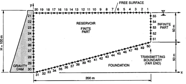
For the purpose of illustration, a simple example is presented in this Appendix.
A two-dimensional infinite reservoir impounded by a straight gravity dam is subjected to
an El Centro horizontal acceleration (file INPSHE INPUT Al). The reservoir is modelled using
55
constant boundary element mesh as shown in Fig. A.l
Fig. A. 1 The Constant Boundary Element Model of Infinite
2D
Reservoir
-
N
=
55
The list of the parameters used
in
the input data file, TESTM INPUT
A1
is as follows:
N
=
55 (elements)
NO
=
20 (last elem. number at the top near a dam)
N1
= 30 (last elem. number at the base of the dam)
N2
=
50 (last elem. number at the base near far end)
NOUT
=
1
(flag for detailed output)
HY
=
50 (height of the infinite part of the reservoir
in
meters)
C
=
1440 (velocity of sound
in
water
in
m/s2)
ALFA =
0.0
(coefficient of reflection in full damping case)
DF
=
0.0 (vertical acceleration of the frst mode at the far end)
Coordinates of the nodal points together with boundary conditions on the dam face and
on the foundation base together with excitation hquencies are listed in a copy of the original
file TESTM INPUT Al.
- 4 -
Listing of
the
file TESTM INPUT
A1
a a a a a a a a a r x a a a a a a a a a a a a a a a aer e a a a aaaer a a a a a a a a a a CT ap: am a a CL
e
a u t x a a a a e a a e a a a a a a p : a a a a a a N N N N N N N N N N N N N N N N N N N N N N N N N N N N N N N N N N N N N N N N N N N N N N N N N N N N N N N N N N N N N N N N m m m m m m m m m m m m m m m m m m=';zm
m m m m m m a m m m m m m m m m m m m m m mz z
m m m m rn m m m m m m m m m m m m m m m m m m m m m m m m m m m m m m mu u u u u u u u u a a
u a a a a a a a a a a a
u a
a u
a a
u u
u u
u u
u u
u u
u a
u u
a u
u a
a u
a a
u u
u u
u u u u u u u u u u u u
a a a u u a a a a a a
N N N N N N N N N N N N N N N N N N N N N N N N N N N N N N N N N N N N N N N N N N N N N N N N N N N N N N N N N N N N N N N N m ~ m m M M M M m m ~ m ~ ~ m m m m ~ m M m M m M m m m M m m m m m M m m m m m m m M Nl M M m m M M M m m M M M M IIl m m m m w m M m m m ama aa(O a a a a a a a a a a am mama am a a a (O a a ma a a a a am a a (D a a a a a ma a a a a ma am a a a a am a a a a ma a a a a ( 0 a a a a a a a (0 (Oaa U U U U U U U U U U U U U U U U U U 0 0 U U U U U 0 U U 0 U U U 0 0 U U 0 0 U 0 U U U U U U U U U U U U U U U U U U U U U U U UB
FILE: TESTM INPUT A 1 NATIONAL RESEARCH COUNCIL OF CANADA...
20 I N F I N I T E RESERVOIR BY THE BEMC 55,20p3Op50pl 5 0 p 1 4 4 0 r 0 . 0 0 ~ 0 . 0 200.0,100.0 190.0p100.0 180.0*100.0 170.0p100.0 160.0,lOO.O 150.0,lOO.O 140.0p100.0 130.0,lOO.O 120.0*100.0 110.0*100.0 100.0*100.0 90.0p100.0 80.0*100.0 70.0p100.0 60.0,lOO.O 50.0p100.0 40.0p100.0 30.0,lOO.O 20.0,100.0 10.0,100.0 0.09100.0 0.0,90.0 0.0,80.0 O.Op70.0 O.Op60.0 0.0,50.0 O.Op40.0 O.Op30.0 0.0*20.0 0.0*10.0 O.O,o.o 10.0p2.5 20.0p5.0 30.097.5 40.0p10.0 50.0p12.5 60.0,15.0 7 0 . 0 ~ 1 7 . 5 80.0,20.0 90.0922.5 100.0,25.0 110.0p27.5 120.0,30.0 . 130.0p32.5 140.0p35.0 150.0137.5 160.0p40.0 170.0p42.5 180.0p45.0 190.0947.5 200.0,50.0 200.0p60.0 VWHPO 4.2 CMS SL422 PAGE 00001 TESOOOlO TES00020 TES0003 TES00040 TES00050 TES00060 TES00070 TES00080 TES00090 TESOOlOO TESOOllO TES00120 TES00130 TES00140 TES00150 TESOOl6O TES00170 TES00180 TESOOl9O TES00200 TES00210 TES00220 TES00230 TES00240 TES00250 TES00260 TES00270 TES00280 TES00290 TES00300 TES00310 TES00320 TES00330 TES00340 TES00350 TES00360 TES00370 TES00380 TES00390 TES00400 TES00410 TES00420 TES00430 TES00440 TES00450 TES00460 TES00470 TES00480 TES00490 TES00500 TES00510 TES00520 TES00530 TES00540 TES00550
r l d r l d d r l d r l r l d 0 0 0 0 0 0 0 0 0 0 c n ~ f n f n c n c n f n c n c n f n W W W W W W W W W W C C C C C C C I - C C 0 0 0
. . .
M M M M M M M M M M M M M M M M M M M M O O O h h h h h h h h h h N N N N N N N ~ N N N W N N N N N N N N ~ a ~ m M M M M M M M M M M h h h h h h h h h h h h h h h h h h h h r ~ m ~ m m ~ ~ m m m ~ ~ d ~ U ~ ~ e e u d ~ d d d d ~ d d u u a ~ e ~ o a a e ~ o ~ ~ d ~ o ~ ~ u ~ o ~ a 0 0 0 d d d d d ~ ~ d d d N N N N N N N N N N N N N N N N N N N N * M O h e O h d r l ~ d d O w N a w N m * ~ m- -
- 0 0 0 0 0 0 0 0 0 0 0 O O O O O O O O O O O O O O O O O O O O r l N N M ~ U Y I ~ ~ h ~ O ~ O O r ( N N M ~ U O O O d d d d r l d r ( r l r ( r ( .. . . - . . .
M * O ~ N ~ O r l ~ h O M \ D o \ N ~ O ‘ N U I ( O d U h 0 0 0 .. . .
. 0 0 0 O O O O O O O O O O O O O O O O O .. . .
. . .
N W N 0 0 0 0 0 0 0 0 0 0 1 1 1 1 1 1 1 1 1 1 1 1 1 1 1 1 1 1 1 I O Q O d ~ d N N N M M M M $ ~ $ $ ~ ~ ~ ~ ~&
FILE: TESTM INPUT A1 NATIONAL RESEARCH COUNCIL OF CANADA
...
VWHPO 4 . 2 CMS SL422 PAGE 00004 TES00900 TES00910 TES00920 TES00930 TES00940 TES00950 TES00960 TES00970 TES00980 TES00990 TESOlOOO TESOlOlO TES01020 TES01030 TES01040 TES01050 TES01060 TES01070 TES01080 TES01090 TESOllOO T E S O l l l O TES01120 TES01130 TES01140 TES01180 TESO119O TES01200 TESOl2lO TES01220I
RRRRRRRRRRR RRRRRRRRRRRR RR RR RR RR RR RR RRRRRRRRRRRR RRRRRRRRRRR RR RR RR RR RR RR RR RR RR RR EEEEEEEEEEEE EEEEEEEEEEEE E E E E E E EEEEEEEE EEEEEEEE E E E E E E EEEEEEEEEEEE EEEEEEEEEEEE SSSSSSSSSS SSSSSSSSSSSS SS
ss
SS SSS SSSSSSSSS SsSSsSsSS SSSss
SS SS sSSsSSSsSSSS ssSSSSSSSS NN NNNNN
NN NNNN NN NNNN
NN NN NN NN NN NN NN NN NN NN NN NNNN NN NNNN NN NNN NN NN NN N CCCCCCCCCC CCCCCCCCCCCC CC CC CC CC CC CC CC CC CC CC CCCCCCCCCCCC CCCCCCCCCC DDDDDDOOD DDDDDDDDDD DO DO DD D D DD DO DD DD DD DD DD DD DD DD DD DD DDDDDOODDO DDODDDDDO SSSSSSsSss SSSSsSsSSSSS SS SS SS SSS SsSSSSSSS sSSSSSSSS SSS SS SS SS SSSSSSSsSSSS SssSSSsSSSFinal Output Graphs from SPLOTN2 FORTRAN A1
The El Centro horizontal component of the acceleration record and the response to it in
the hydrodynamic: pressures (hydrodynamic pressure history) and other graphs.
a,
= 0.00 (full damping)
NT
=
4096
(number of points in the acceleration record and also number of steps used in the
FFT
analysis)
Aw
= 0.3068 rad/s (frequency step)
The El Centro component was recorded during the Imperial Valley earthquake in
California on May 18, 1940. It
had
a magnitude of M6.6. The measured peak acceleration was
PHA
=
-3.41705
m/s2 and number of points in the record was equal to 2687.
TAG DATA:
DR. ALEXANDER
M. JABLONSKI RM 151 M-20
USERID:
ALEXNMP
DEVICE:
221LASER
DIST:
JABLONSK
TYPE:
PLOT-POP <THICKPEN 2>
FILEID:
D U M 2
PLOTFILE
A4
FORM:
PAPER11
SPOOLID:
4366
CLASS:
A
SYSTEM:
NRCVMOl
COPY:
1
I
O'E
0 -0*
0- 0
m
9
-
0 02 0- 0
39
I I I I I v I I 1 I I I I 0I
HARM. R E S P O N S E
-
R E A L PART
MAX
=
0.05
.
AT
X
=
0.05
MIN
=
0.00
AT
X
=
0.00
0I
I
I 1 I 1 I0.0
I1
.o
2.0
I3.0
I I4.0
5.0
7.0
8.0
9.0
I6.0
110.0
FREQUENCY
HZ
I
I I I I02'0
ST '0
OT'O
SO'O
00'0
3380tI
'.LvLs/~~~~oJ
I
I I ISO'O-
OT'O-
ST'O-
02'0-
'tl(lbH
?V.LOL
9
-0 -49
-09
- a
0- &
0- c d
Is
*
U
9 2
- m
W
5
m
W
P=
o h
- 4
0 - c i 0- 4
0 - 4 0 0HARM. R E S P O N S E
-
ABS. VALUE
MAX
=
0.05
AT
X
=
2.64
MIN
=
0.00
AT
X
=
0.00
0
1
I
I 1 I I I I0.0
1.0
5.0
6.0
7.0
I2.0
I3.0
I4.0
I I8.0
9.0
10.
FREQUENCY
HZ
I 1 I Z I I I I I