HAL Id: hal-01159677
https://hal.inria.fr/hal-01159677
Submitted on 3 Jun 2015
HAL is a multi-disciplinary open access
archive for the deposit and dissemination of
sci-entific research documents, whether they are
pub-lished or not. The documents may come from
teaching and research institutions in France or
abroad, or from public or private research centers.
L’archive ouverte pluridisciplinaire HAL, est
destinée au dépôt et à la diffusion de documents
scientifiques de niveau recherche, publiés ou non,
émanant des établissements d’enseignement et de
recherche français ou étrangers, des laboratoires
publics ou privés.
Fast and high quality topology-aware task mapping
Mehmet Deveci, Kamer Kaya, Bora Uçar, Umit Catalyurek
To cite this version:
Mehmet Deveci, Kamer Kaya, Bora Uçar, Umit Catalyurek. Fast and high quality topology-aware
task mapping. 29th IEEE International Parallel & Distributed Processing Symposium, May 2015,
Hyderabad, India. �hal-01159677�
Fast and high quality topology-aware task mapping
Mehmet Deveci∗, Kamer Kaya†∗, Bora Uc¸ar‡, ¨Umit V. C¸ ataly¨urek∗
∗Biomedical Informatics, The Ohio State University, Columbus, OH
{mdeveci,kamer,umit}@bmi.osu.edu
†Computer Science and Engineering, Sabancı University, Istanbul, Turkey
‡CNRS and LIP (UMR 5668), ENS, Lyon, France
Abstract—Considering the large number of processors and the size of the interconnection networks on exascale-capable supercomputers, mapping concurrently executable and communicating tasks of an application is a complex problem that needs to be dealt with care. For parallel applications, the commu-nication overhead can be a significant bottleneck on scalability. Topology-aware task-mapping methods that map the tasks to the processors (i.e., cores) by exploiting the underlying network information are very effective to avoid, or at worst bend, this limitation. We propose novel, efficient, and effective task mapping algorithms employing a graph model. The experiments show that the methods are faster than the existing approaches proposed for the same task, and on 4096 processors, the algorithms improve the communication hops and link contentions by 16% and 32%, respectively, on the average. In addition, they improve the average execution time of a parallel SpMV kernel and a communication-only application by 9% and 14%, respectively.
Keywords-Task mapping, communication graph, partitioning
I. INTRODUCTION
For parallel computing, task mapping has a significant im-pact on the performance, especially when supercomputers with hundreds of thousands or millions of processors shoulder the execution. It is usually the case that the communication pattern between the tasks has already been designed to minimize pos-sible performance bottlenecks, such as high number of mes-sages or communication volume, via tools such as graph and hypergraph partitioners, e.g., [1], [2], [3], [4], [5]. However, this effort alone is not sufficient, since the mapping-based met-rics such as the maximum link congestion and the total number of hops the messages travel in the network can also be signifi-cant bottlenecks on the performance. This is especially true for today’s supercomputers with large-diameter interconnection networks, and concurrent and non-uniform job submissions yielding sparse and wide-spread processor allocations for par-allel applications. There exist various studies in the literature which analyze the impact of task-to-processor mappings on the parallel performance [6], [7], [8], [9] and report significant speedups, e.g., 1.64X [10], just with an improved mapping.
There are two main research directions for mapping. The first one focuses on block-based processor allocations, e.g., the ones on IBM BlueGene [8], [10], [11], [12], [13]. The second direction focuses on sparse allocations in which the allocated processors are not contiguous within the network [14], [15]. This direction is more general: sparse allocations have been
used in various parallel systems, and the mapping algorithms based on this model can also be used for the block-based model. In this work, we follow the second direction.
The problem of finding an optimal task-to-processor mapping is NP-complete [15], and various heuristics have been proposed [16], [17], [18], [19]. Many of these heuristics use graphs and related combinatorial structures to model the task interactions as well as the network topologies. For example, the open-source mapping library LibTopoMap [15] uses a task graph and network topology information. The task graph is first partitioned into the number of allocated nodes, and various graph-based algorithms are used to map the tasks to the allocated processors. Other libraries such as JOSTLE [20] and Scotch [1] also exist. These two libraries apply simultaneous partitioning and mapping of the task and topology graphs.
A good mapping algorithm must be able to provide high-quality task-to-processor mappings. It also needs to be efficient in order not to intervene the supercomputer’s performance. We follow these two important criteria and propose novel, very efficient, refinement-based mapping algorithms. We show that they can produce high-quality mappings w.r.t. the topology-related metrics such as the average link congestion and the total hops the messages take. We compare the performance of the proposed algorithms with that of LibTopoMap and Scotch. The experiments on a supercomputer with a 3D torus network and 4096 processors show that the algorithms can improve the
weighted hop and the maximum congestion (that will be
de-scribed below) by 16% and 32% on the average, respectively, compared to the default mapping. These metric improvements yield a 43% performance improvement on one case for a
synthetic, communication-only application (Figure 4b–PATOH)
and a 23% improvement on the performance of a sparse-matrix
vector multiplication (SpMV) kernel (Figure 5–METIS).
Overall, with 4096 and 8192 processors, they improve the performance of a parallel SpMV kernel and a communication-only application by 9% and 14%, respectively (Table I).
The organization of the paper is as follows. In Section II, the background for the topology-aware task mapping is given. We also summarize the related work and the target architecture in this section. In Section III, we present three mapping algorithms minimizing various metrics. Section IV presents the experimental results, and Section V concludes the paper.
II. BACKGROUND
Let Gt= (Vt, Et) be a directed MPI task graph, where Vt
is the task set, and Et is the edge set modeling task-to-task
communications, i.e., (t1, t2) ∈ Et if and only if t1 ∈ Vt
sends a message to t2 ∈ Vt. Let Gm = (Vm, Em) be the
network topology graph where Vm is the set of computing
nodes equipped with many processors/cores, and Em is the
edge set modeling the physical communication links between
the nodes, i.e., (m1, m2) ∈ Em if and only if m1 ∈ Vm
and m2 ∈ Vm have a link in between. Let Va ⊆ Vm be the
set of computing nodes reserved for the application. The topology-aware mapping problem can be defined as finding a
mapping function (Γ : Vt → Va) that minimizes the parallel
execution time. For a task set S ⊆ Vt, we use Γ[S] to denote
the node set to which the tasks in S are mapped to.
There are two well-received metrics to model the network
communication overhead. The total hop count (TH), which
is the total length of paths taken by communication packets, is a latency-based metric. The maximum message
congestion (MMC), which is the maximum number of
messages sent across a link. We assume that the messages are not split and sent through only a single path via static routing.
Let Γ be a given mapping where m1= Γ(t1) if and only
if t1 is assigned to one of node m1’s processors. Then
TH(Γ) = X
(t1,t2)∈Et
dilation(t1, t2),
where dilation(t1, t2) = SPL(Γ(t1), Γ(t2), Gm) which is the
shortest-path length between Γ(t1) ∈ Vmand Γ(t2) ∈ Vm.
Let the congestion on a network link e ∈ Embe
Congestion(e) = X
(t1,t2)∈Et
inSP(e, Γ(t1), Γ(t2), Gm), (1)
where, inSP = 1 if and only if e is on the shortest path
between Γ(t1) and Γ(t2), and 0 otherwise. Therefore, a link’s
congestion is equal to the number of messages that passes through it. Hence, the maximum message congestion is
MMC(Γ) = max
e∈Em
{Congestion(e)}.
The above metrics assume unit communication costs and link capacities. In order to handle heterogeneous costs and bandwidths, the task and topology graph models are extended
as follows. Each edge e0 ∈ Etin the task graph is associated
with a cost c(e0) that corresponds to the communication
volume sent/received between the tasks. Similarly, each link
e ∈ Em in the topology graph is associated with a
com-munication capacity bw(e) that corresponds to the link band-width. Moreover, for further heterogeneity support, each node
m ∈ Vmis associated with a computation capacity w(m) that
corresponds to the number of available (allocated) processors
in m. All the nodes that are not in Va have zero capacity.
Based on these attributes on the edges, the weighted hop (WH)
metric, i.e., the total number of hops taken by each packet, is
WH(Γ) = X
(t1,t2)∈Et
dilation(t1, t2)c(t1, t2).
We define the volume congestion (VC) of a link e ∈ Emas
VC(e) = P
(t1,t2)∈Et
inSP(e, Γ(t1), Γ(t2), Gm)c(t1, t2)
bw(e)
which is the ratio between the overall volume of the communication passing from e and its bandwidth. Then, the
max volume congestion (MC) metric is the congestion of the
bottleneck link in the network with the maximum VC value. A communication-bounded parallel application can be ei-ther latency-bounded or bandwidth-bounded depending on the communication pattern. For example, applications with frequent communication steps and small messages are likely to be latency-bounded, while those with larger messages are likely to be bandwidth-bounded. For latency-bounded
applications, TH and WH metrics can better correlate with
the communication overhead. On the contrary, MMCand MC
are better choices for the bandwidth-bounded applications. Depending on the communication pattern, it might be better to
minimizeMC(MMC) in the expense of an increase onWH(TH),
or vice versa. However, it is indeed difficult to find a consensus between these metrics. Therefore, here we define average
mes-sage congestion (AMC) and average congestion (AC) metrics
to account for both number of hops and congestion. Let Emt
be the set of the links that are used throughout the execution of the parallel application. The message and volume based average link congestions over the used links can be defined as
AMC(Γ) = P e∈EmCongestion(e) |Et m| , AC(Γ) = P e∈EmVC(e) |Et m| Since TH = P
e∈EmCongestion(e), AMC is the ratio of
TH to the total number of links used during the application.
Similarly, AC is related to the ratio of WH to the number of
links used during the execution (they are equal only when the communication links have unit bandwidths).
The communication during the execution is a real-time pro-cess that can easily be affected by many outside factors (e.g., network traffic and overhead from competing jobs). Hence, the theoretical metrics given above can only approximate the actual overhead. In Section IV-E, we will discuss and evaluate the interplay of these metrics on the performance. A. Related Work
Existing mapping algorithms can be divided into two classes: single-phase and two-phase methods. The algorithms in the former class perform simultaneous partitioning and mapping using the task and topology graphs, whereas those in the latter partition the task graph in the first phase and map the parts to the processors in the second one.
Pellegrini and Roman [21] proposed a single-phase recursive-bipartitioning algorithm for various topologies. Wallshaw and Cross [20] proposed a multilevel partitioning algorithm which performs mapping in the initial partitioning and refinement phases.
The two-phase mapping methods make an abstraction of the partitioning phase and work with a pre-partitioned task set. These studies can be divided into two based on the task-dependency model and network topology. The first set adapts geometric task-interaction models, e.g., [22], [23] on IBM’s BlueGene systems with block-based node allocations and on sparse allocations [14]. Still, most of the work focuses on the connectivity-based models, specifically graph models. This problem is shown to be NP-complete [15], [24], and many heuristics exist in the literature, e.g., [16], [17], [18], [19]. In this work, we investigate a two-phase graph-based approach. B. The architecture
Six of the top ten supercomputers in the Top500 list (June 2014), have torus networks (one 3D, four 5D, one 6D). In this work, we target NERSC’s Hopper supercomputer with Cray XE6’s 3D torus. The network has Gemini routers directly connected to two computing nodes. Each router is associated with a coordinate on x, y, and z dimensions, and connected to all six neighbor routers. The torus network provides wrap-arounds, and the messages between the nodes are statically routed following the shortest paths. The network links have different bandwidth values on various dimensions. On Cray systems, the scheduler allocates a non-contiguous set of nodes for each job [25]. Although it attempts to assign nearby nodes, no locality guarantee is provided. The topology information, e.g., the routers’ coordinates and connections, as well as link bandwidths, can be captured using system calls (rtr), and a static topology graph can be obtained. During runtime, each MPI process can obtain its node id, and the vertices in the topology graph can be associated with the computational units.
In Hopper, the network latencies for the nearest and farthest node pairs are 1.27µs and 3.88µs, respectively. The link bandwidths vary from 4.68 to 9.38 GB/sec. Ideally, reducing the hop counts between the communicating tasks lowers the overhead. But when there are many communicating tasks, a link can be congested due to the communication pattern, which might cause communication stalls and harm the performance. Still, thanks to static routing, the congestion can be measured and optimized accurately.
III. FAST ANDHIGHQUALITYMAPPINGALGORITHMS
We propose three mapping algorithms to minimize WHand
MC. Here we will describe these algorithms. Their adaptation
for TH and MMC is trivial. Among them, the ones that
minimize WH can be applied to various topologies, whereas
those minimizing MC require static routing.
A. A Greedy mapping algorithm
The first algorithm Greedy Mapping given in Algorithm 1
finds a mapping Γ : Vt → Vm to minimize WH. It uses the
task graph Gtand the topology graph Gm. The algorithm is
similar to greedy graph growing, and initially maps NBF S
seed task vertices to the nodes. It assumes a symmetric Gt
while finding the neighbors of a given task since WH is an
undirected metric, i.e., the number of hops between m1 and
m2is the same regardless of direction.
Algorithm 1: Greedy Mapping
Data: Gt= (Vt, Et), Gm= (Vm, Em): task and topology
graphs, NBF S: # vertices to be initially mapped
connt← 0 for each t ∈ Vt I initialize the max-heap
Γ[t] ← −1 for each t ∈ VtI initialize the mapping
I Find the task with M SRV t0 ← tM SRV
I Map t0 to an arbitrary node
Γ[t0] ← m0
I Update connectivity for the tasks in nghbor(t0)
for each tnin nghbor(t0) do
conn.update(tn, c(t0, tn))
while there is an unmapped t do
if number of mapped tasks < NBF S then
tbest← the farthest unmapped task I found by BFS
else
tbest← conn.pop() I the one with maximum conn.
1 mbest←GETBESTNODE(tbest, Gm, Gt, Γ, conn)
Γ[tbest] ← mbest
for each tnin nghbor(tbest) do
2 conn.update(tn, c(tbest, tn))
Throughout the algorithm, the total connectivity of each task to the mapped ones are stored in a heap conn. The
algorithm first maps the task tM SRV with the maximum
send-receive communication volume to an arbitrary node. Until all tasks are mapped, the algorithm gets an unmapped
task from conn after all the NBF S seeds are mapped.
Otherwise, the farthest task to the set of mapped tasks is
found by a breadth-first search (BFS) on Gt where all the
mapped tasks are assumed to be at level 0 of the BFS. Ties are broken in the favor of the task with a higher
communication volume. If Gt is disconnected, a task with
the maximum communication volume from one of the
disconnected components is chosen. Once tbest is found, its
best node is obtained byGETBESTNODE. If tbestis connected
to none of the mapped tasks, GETBESTNODE performs a
BFS on Gm to return one of the farthest allocated nodes to
the set of the non-empty nodes, i.e., the ones with a mapped
task. Otherwise, if tbest is connected to at least one of the
mapped tasks, a BFS on Gm is performed from the nodes to
whom one of the nghbor(tbest) is mapped (again assuming
these nodes are at level 0). As an early exit mechanism, a BFS stops when the empty nodes (without a mapped task) are found at a BFS level. Then among these empty nodes, the one
with the minimum WH overhead is returned. Therefore, the
algorithm performs multiple BFS executions on Gtand Gm.
For simplicity, the description above assumes one-to-one
task-to-node mapping, i.e., |Vt| = |Va|. In reality, each node
has multiple processors, so multiple tasks can be assigned to a single node. These cases can be addressed by using the
com-putation loads and capacities, and modifyingGETBESTNODE
so that it returns only a node with some free capacity. Another common solution is using traditional graph partitioning as a preprocessing step to reduce the number of tasks to the number
of the allocated nodes while minimizing the edge-cut [15].
We follow this approach and use METIS [3] to partition Gt
into |Va| nodes, where the target part weights are the number
of available processors on each node in Va. Since graph
partitioning algorithms do not always obtain a perfect balance, as a post processing, we fix the balance with a small sacrifice on the edge-cut metric via a single Fiduccia-Mattheyses (FM) iteration [26]. When the number of processors in the nodes are not uniform, we map the groups of tasks with different weights at the beginning of the greedy mapping since their nodes are almost decided due their uniqueness.
In the algorithm, NBF S controls the number of initial seed
mappings. A large NBF S distributes the loosely connected
components of the task graph to the nodes that are farther from each other. However, this will not work well for the task graphs with a low diameter. In our implementation, we use
NBF S ∈ {0, 1} to generate two different mappings and return
the one with the lower WH.
The complexity of the algorithm is dominated by the operations at lines 1 and 2. Each update of the heap (line 2)
takes O(log |Vt|) time, and this line is executed at most
|Et| times, yielding O(|Et| log |Vt|). The BFS operation in
GETBESTNODE has O(|Em|) cost, yielding an overall
com-plexity of O(|Vt||Em|). For a task tbest and a candidate node
at the last level of the BFS performed in GETBESTNODE, the
cost of computing the change on WH is proportional to the
number of edges of tbest(the hop count between two arbitrary
nodes can be found in O(1), since Gm’s are regular graphs).
Since there are at most |Va| = |Vt| candidate nodes and |Et|
edges, the complexity of this part throughout the algorithm
is O(|Vt||Et|). Therefore, the complexity of Algorithm 1 is
O(|Vt|(|Em| + |Et|))—in practice it runs faster thanks to the
early exits in GETBESTNODE BFSs.
B. A Refinement algorithm for the weighted hop
Algorithm 1 is our main algorithm and the other two will refine its mapping. Even after its execution, it is possible to
improve WH via further refinement. We have implemented a
Kernighan-Lin [27] type algorithm which uses “task swaps” to
refineWH(Algorithm 2). It gets a Γ, Gt, and Gmas input and
modifies Γ to lower theWHmetric. Similar to greedy mapping,
for simplicity, Algorithm 2 assumes that Gtis symmetric and
Γ is a one-to-one mapping between the tasks and nodes. The algorithm selects a pair of task vertices and swaps them
to improve WH. The first task twh is chosen using a
max-heap, whHeap, which initially organizes the tasks w.r.t. the
WHamount they incur computed by a functionTASKWHOPS
function (line 1). Hence, twh is the task individually
re-sponsible for the largest WH. Choosing the second task for
the swap operation is more complicated; a naive approach
that considers to swap twh with all the other tasks requires
O(|Vt|2) comparisons. In order to avoid this cost, we have
implemented a BFS-based task-selection algorithm. A simple
observation is that to reduce WH, twh needs to move closer
to its neighbor tasks. Therefore, we perform a BFS on Gm
starting from the nodes which have a neighbor of twh, i.e., the
Algorithm 2: WH Refinement
Data: Gt= (Vt, Et), Gm= (Vm, Em), Γ, ∆
I compute the currentWHforΓ
WH←CALCULATEWEIGHTEDHOPS(Gt, Gm, Γ)
whileWHis improved do
I computeWHincurred by each task I place the tasks in a max-heap whHeap
1 for t in Vt do
wht←TASKWHOPS(t, Gt, Gm, Γ)
whHeap.insert(t, wht)
2 while whHeap is not empty do
twh← whHeap.pop()
3 for the first ∆ nodes m ∈ Vavisited in the order of
the BFS from Γ[nghbor(twh)] do
t ← the task mapped to m
4 if swapping twhand t improves WHthen
Γ[t] ← Γ[twh]
Γ[twh] ← m
5 Update whHeap for neighbors of twh
6 Update whHeap for neighbors of t
break
nodes in Γ[nghbor(twh)] (these are the level 0 nodes of BFS).
Whenever a Va node with a the task t is found, theWHvalue
after the potential Γ[twh] ↔ Γ[t] swap operation is computed.
The actual swap is performed as soon as this computation
reveals an improvement onWH. Since the likelihood of a WH
improvement decreases when we go deeper on the BFS tree, we use an early exit mechanism to avoid a full BFS traversal of
Gm. Here we give an example to clarify the statement, assume
c(e) = 1 ∀e ∈ Et. If the maximum hop count between Γ[twh]
and Γ[nghbor(twh)] is d then when twh is moved to a node
after the BFS level d,WHincurred by twhcannot be improved.
Furthermore, when we go deeper in the BFS, twh’s incurred
WHvalue will increase. Even in this case, the overallWHmay
still be improved due to the reduction of WHincurred by the
second task t. However, this is less likely to happen
consid-ering Γ[t] is handpicked for twh but Γ[twh] is only a random
node for t. The early exit mechanism reduces the number of
considered swap operations that are unlikely to improveWH. In
Algorithm 2, a parameter ∆ is used as an upper bound on this
number. If ∆ operations are checked for twh, the algorithm
continues with the next whHeap vertex. A refinement pass is completed when whHeap is empty, and the next pass is performed only if there is an improvement in the previous pass.
The complexity of the loop at line 1 is
O(|Vt| log |Vt| + |Et|). The loop at line 2 iterates |Vt|
times. The complexity of the BFS operation at line 3
is O(|Em|) and it is also performed |Vt| times. The
complexity of the swap operation and the calculation of
new WH at line 4 is proportional to the total number
of edges of twh and t for each candidate node. Since
there are at most ∆ candidate nodes for each BFS, the
complexity of line 4 for each pass becomes O(∆|Et|).
Lines 5 and 6 are executed at most once for each vertex
Therefore, the overall complexity of the algorithm becomes,
O(|Vt| log |Vt| + |Et| + |Em||Vt|+∆|Et| + |Et| log |Vt|).
The most dominant factor is the complexity of the BFS
operations which is O(|Em||Vt|). Fortunately, the practical
execution time is very low, since we stop after ∆= 8 swap candidates. We experimented with other exit mechanisms based on the maximum BFS level instead of the number of swap operations, and the preliminary experiments favored the approach described above. Furthermore, we observed that
most of the improvement in WHis obtained after only a few
passes. Hence, in order to be more efficient, we perform a pass
only if WHis improved more than 0.5% in the previous one.
Similar to that of Algorithm 1, the description above assumes a one-to-one task-to-node mapping and performs the refinement on the node level, i.e., by swapping the vertices representing a group of tasks. With slight modifications, it can perform the refinement on the finer level task vertices or in a multilevel fashion from coarser to finer levels. In our experiments we choose to perform only on the coarser task
graphs we obtained after METIS, since with WH-improving
swap operations on the finer level, the total internode commu-nication volume can also increase and the performance may decrease. Although this increase can also be tracked during the refinement, we do not want to sacrifice from the efficiency. C. A Refinement algorithm for the maximum congestion
Although Algorithms 1 and 2 significantly improve WH,
they can negatively affectMCorMMC, and this can degrade the
performance especially for the bandwidth-bounded applica-tions. Therefore, we propose another refinement algorithm
(Al-gorithm 3), which improves the MC metric with minimal WH
damage (adapting this algorithm to refine MMC is trivial).
The algorithm can accurately model and minimizeMC for the
interconnection networks with static routing. We will discuss the required enhancements for the dynamic-routing networks.
Algorithm 3: MC Refinement
Data: Gt= (Vt, Et), Gm= (Vm, Em), Γ, ∆
I calculate initial max and average congestions MC,AC← calculateCongestion(Gt, Gm, Γ)
I initialize the link congestion heap
I store the tasks whose messages goes through links congHeap, commT asks ←INITCONG(Gt, Gm, Γ)
whileMC orACis improved do
1 emc← congHeap.pop()
2 for tmc∈ commT asks[emc] do
3 for the first ∆ nodes m ∈ Va visited in the order of
the BFS from Γ[nghbor(tmc)] do
t ← the task mapped to m
if swapping tmc and t improvesMC orACthen
Γ[t] ← Γ[twh]
Γ[twh] ← m
Update congHeap for tmc and t edges
Update commT asks for tmcand t edges
goto line 1
The algorithm gets a Γ, Gm, and Gt and modifies Γ to
find mapping with a better congestion. First, it computes the
initial congestion of Γ, and initializes the congHeap using
an INITCONG function. This max-heap stores the topology
graph edges w.r.t. their congestion values. The algorithm also initializes commT asks, that is used to query the tasks whose messages go through link e, i.e., commT asks[e]. Since, a message can go at most D (network diameter) hops, the
maximum size of commT asks becomes |Et|D, which is
manageable since D is not a large number.
After the initialization, the algorithm finds the most
congested link emc. Then for each tmc∈ commT asks[emc],
the node to which tmc will be moved is sought via BFS
traversals on Gm starting from the nodes Γ[nghbor(tmc)].
The second task t to swap is chosen from the tasks of the Va
nodes traversed during the BFSs. This BFS order is important
to have a minimal damage on WH. For each such candidate
node, a virtual swap operation is performed to compute new
MC and AC values. As soon as an improvement is detected,
the actual swap operation is performed, and the execution continues with the next congested link. Whenever a vertex is moved, updates on the congHeap and commT asks are
performed for all the incoming and outgoing edges of tmc
and t in Et. If there is no improvement after ∆= 8 trials,
the early exit mechanism terminates the inner for loop. Then,
the next task in commT asks[emc] is chosen and the search
restarts. If no improvement is found for the most congested link the algorithm stops. This algorithm can be applied both to coarser and finer task graphs. However, we only apply it on the coarser graph due to the reasons explained before.
With static routing, a message route can be found in O(D) time. The congestions of all the links can be calculated in
O(D|Et|) time, and the cost of initializing congHeap is
O(|Em| log |Em|). A task insertion to a commT asks set
(implemented as a red-black binary tree using std:set in
C++) can be done in O(log |Vt|). Since each message (an
edge in Et) can pass through at most D links, the complexity
of commT asks’s initialization is O(D|Et| log |Vt|).
Therefore the initialization phase has a complexity of
O(D|Et| log |Vt| + |Em| log |Em|). A refinement pass starts
at line 2. The main for loop iterates at most |Vt| times
and the complexity of a BFS at line 3 is O(|Em|). Hence,
the overall BFS complexity in a pass is O(|Vt||Em|). For
each candidate swap operation, we compute MC and AC
by temporarily updating congHeap where an update costs
log |Em| and a candidate swap requires at most D updates
for each of the tmcand t edges. Since we consider at most ∆
swap operations for a tmc which can be any vertex in Vt, the
cost of MC and AC computation is O(Et ∆ D log |Em|) for
each emc. Once an improvement is found, the data structures
congHeap and commT asks are updated and this happens only once per pass (a while loop iteration). Hence, the overall
complexity of a pass is dominated by the BFS and MC–AC
computations. Therefore the overall complexity of a pass
becomes O((Et ∆ D log |Em|) + (|Vt||Em|)).
Algorithm 3 accurately sees the maximum congestion on a static-routing network. For the networks with dynamic routing, an approximate refinement algorithm with a similar structure
can be used. For example, the bandwidth on the Blue Gene/Q and Blue Gene/P can be maximized by placing the heavily communicating tasks to the diagonals of the torus [22], [23].
IV. EXPERIMENTS
In order to evaluate the quality of the mapping algorithms,
we conducted various experiments on two irregular
applications, an SpMV kernel and a synthetically generated application. The proposed methods are implemented in the
UMPA framework. The UG and UWH variants minimize WH
using Algorithms 1 and 2, and UMC and UMMC minimizesMC
and MMC, respectively using Algorithm 3 (we do not give
the results for TH variant as they are very close to those of
UG and UWH). These mapping methods are compared against
the default MPI mapping (SMP-STYLE) in Hopper (DEF),
the mapping provided by SCOTCH (SMAP, version 5.1.0 as
the newer one does not support sparse allocations) [1], and
the ones provided by LibTopoMap (TMAP) [15].
We selected 25 matrices from University of
Florida (UFL) sparse matrix collection, belonging to 9 different classes (the list is at the supplementary page:
http://web.cse.ohio-state.edu/∼deveci/umpamap). We used 7
graph and hypergraph partitioners to partition these matrices: SCOTCH [1], KAFFPA (KAHIP) [2], METIS [3], PATOH [4],
and UMPA [5]. A summary of the partitioning results are
given in Section IV-A. MPI task communication graphs corresponding to these partitions are created and mapped to real processor allocations in Hopper. The analysis of the metrics and algorithm efficiency is presented in Section IV-B. Section IV-C analyzes the impact of the mapping algorithms on the communication time, whereas Section IV-D evaluates
the performance improvements for a Trilinos SpMV
kernel [28]. We analyze the impact of the partitioning and mapping metrics on the parallel performance in Section IV-E. A. Partitioning results
The matrices are first converted to a column-net hypergraph model, i.e., the rows represent the tasks with loads proportional to their number of non-zeros. The columns represent sets of data communications where each message has a unit commu-nication costs. On these matrices we perform 1D row-wise par-titioning for 1024, 2048, 4096, 8192 and 16384 parts (we only use 19 matrices for 16384 parts; balanced partitions were not
feasible for the remaining 6). The graph partitioners, SCOTCH
and KAFFPA, are run to minimize the edge-cut, and METIS
and PATOH are run to minimize the total communication
volumeTV. Being a multi-objective partitioner, UMPAis used
with different metrics: UMPAMV minimizing maximum send
volume (MSV) andTV; UMPAMMminimizing maximum
num-ber of sent messages (MSM), total number of messages (TM)
and TV; UMPATM minimizing TM and TV; as their primary,
secondary, and tertiary objectives, respectively [5]. All the partitioners are run with their default parameters.
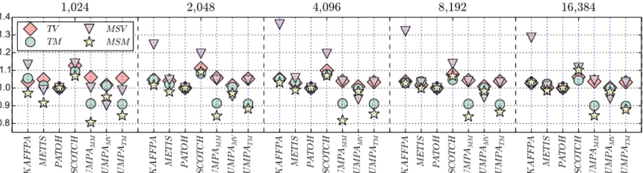
Figure 1 shows the mean metric values normalized with that
metric value of PATOH. Overall, all the tools obtain similar
results, but edge-cut minimizing ones, SCOTCHand KAFFPA,
obtain a slightly worse communication volume quality. For
the MSVmetric, UMPAMV has the best results, e.g., it obtains
a 5–10% better averageMSVvalue w.r.t. PATOHwhich obtains
the best results for TV. For the message metrics, UMPAMM
obtained a 16–19% betterMSM value, and UMPATM obtained
a 9–10% betterTMvalue. These numbers are not given here to
compare the partitioners since the experiment is not designed for that purpose. We want to better understand the impact of the partitioning and mapping metrics on the execution time. B. Mappings on Hopper
Here we evaluate the mapping metric results on Hopper, which has a 3D Torus network and 24 processors per node. Even though the proposed algorithms do not have constraints on the number of processors, we tested them on numbers that are powers of two. Using all the processors in a node results in non-uniform processor allocations per node (since 24 does not divide 1024), in which case we experienced a few failing algorithms in LibTopoMap. Therefore, we used 16 processors per node (4 processors per NUMA domain).
We create directed task graphs by running all the partitioners on each matrix; for each graph and part number, we have
7 MPI task graphs. We will refer a task graph as GX
t when
the part vector obtained from the partitioner X is used to create it. The mapping algorithms are then used to map these graphs to 5 different Hopper processor allocations. Figure 2 shows the average metric values of all mapping algorithms
normalized to those of the default mapping on GPATOH
t graphs.
Almost all algorithms have their best WH andMC values on
GPATOH
t , and bestTHandMMCvalues on G
UMPATM
t . The results
are expected for WH and TH, since WH is closely related to
the communication volume, andTHis related to total number
of messages. On the other hand, it is expected to have better
MC and MMCvalues on the task graphs with lower MSV and
MSM values, respectively. However, in our experiments, we
see a better correlation of these metrics withTV andTM.
In Fig. 2, the DEFmapping obtains already good results on
WHandTH. This is due to the part ID assignment in
recursive-bisection-based partitioners and the placement mechanism in Hopper: the partitioner puts highly communicating tasks to the parts with closer IDs. On the machine side, Hopper places the consecutive MPI ranks within a single node, then it moves to the closer nodes using space filling curves. Therefore, highly communicating consecutive MPI ranks are placed fairly close to each other. However, there is still room for improvement when we exploit the actual task communication
requirements. For example, UG obtains 5–18% and 5–17%
better values on WHandTH, respectively.
Metric improvements on more sparse allocations (with less
number of processors) are higher: UG significantly reduces
WH andTH, and UWH improves them by another 4–5%. Also
the variants that improve theWHmetric also improveMCand
MMC. For example, UG (UWH) improvesMCby 4% (10–12%)
on 1024 and 2048 processors. However, when the number of
processors is high, they increase the MC metric by 13–36%
K A FF PA M E TI S PA TO H SC O TC H UM PA M M UM PA M V UM PA TM K A FF PA M E TI S PA TO H SC O TC H UM PA M M UM PA M V UM PA TM K A FF PA M E TI S PA TO H SC O TC H UM PA M M UM PA M V UM PA TM K A FF PA M E TI S PA TO H SC O TC H UM PA M M UM PA M V UM PA TM K A FF PA M E TI S PA TO H SC O TC H UM PA M M UM PA M V UM PA TM 0.8 0.9 1.0 1.1 1.2 1.3 1.4 TV TM MSVMSM
1
,
024
2
,
048
4
,
096
8
,
192
16
,
384
Fig. 1:Geometric means of the partition metrics w.r.t PATOHfor the corresponding part number.
D T S G W H M C M M C D T S G W H M C M M C D T S G W H M C M M C D T S G W H M C M M C D T S G W H M C M M C 0.6 0.8 1.0 1.2 1.4 1.6 TH WH MMC MC
1
,
024
2
,
048
4
,
096
8
,
192
16
,
384
Fig. 2:Mean metric values of the algorithms on GPATOH
t graphs normalized w.r.t. those of DEF. The numbers at the top denote the number of
the processors, and the letters at the bottom correspond to the mapping algorithms DEF, TMAP, SMAP, UG, UWH, UMC, UMMC, respectively.
1,024 2,048 4,096 8,192 16,384 0.1 0.2 0.3 0.4 0.5
0.13
0.16
0.21
0.31
0.49
0.02
0.03
0.07
0.13
0.28
0.01
0.03
0.05
0.11
0.27
0.02
0.03
0.06
0.13
0.29
0.04
0.08
0.12
0.19
0.37
0.05
0.08
0.13
0.20
0.36
TMAP SMAP UG UWH UMC UMMCFig. 3: (Geometric) mean execution times of different mapping
algorithms on PATOH partitions. The time of UWH, UMC, and UMMC
includes UGtime, as they run on top of it.
TH, and WH except UG on 16, 384 processors. Also, UMC
significantly reduces (27–37%) theMCmetric for all cases and
have 1–13% improvement on WH and TH. Similarly, UMMC
reducesMMCby 24–37% with small increases onTHandWH.
LibTopoMap provides six algorithms, and the best one in our experiments employs recursive graph bi-partitioning. Here
we only present the best variant’s performance (TMAP or T).
The primary metric for LibTopoMap is MC. If TMAP’s MC
value is not smaller than the DEFmapping, it returns the DEF
mapping. Overall, TMAP improves MC by 1–7% with 1–5%
increase on the other metrics. On the other hand, SMAP’s
results are worse than DEFmappings for most of the cases.
Figure 3 presents the (geometric) mean mapping times of
the algorithms. The times of the SMAP, UG and UWH are the
lowest, and they are followed by UMC and UMMC. TMAP’s
execution time is more than the other methods, and it is
1.3–2.6 times slower than the slowest UMPA variant.
C. Communication-only experiments
In task mapping, the communication is usually modeled by assuming all the messages are transferred at once. However,
this may not be the case in practice: load imbalance can delay some transfers, and applications might be using common tech-niques such as communication-computation overlap to hide the latency. Hence, improvements due to mapping may not be visible on an application’s execution time. Here, to limit the impact of these factors, we generate irregular, communication-only applications based on the SpMV communication patterns of the two largest matrices in our dataset: cage15 and
rgg_n_2_23_s0(in short rgg). In this SpMV-like
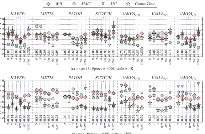
execu-tions, no computation is performed, and all the transfers are initialized at the same time where each processor follows the pattern in the corresponding communication graph. Therefore the total execution time of this application is equal to its communication time. To make the improvements more visible and reduce the noise, we scale the message sizes by using the factors 4K and 256K for cage15 and rgg, respectively. The experiment is performed with 4096 processors. Each mapping algorithm is run with the 7 communication graphs (one per partitioner), and for each mapping, the execution is repeated 5 times to reduce the noise on the time. Figure 4 shows the nor-malized mean execution times with standard deviations and the metric values ( In real case, link congestions are also affected by the other running jobs. The reported congestion-metrics refer to those only incurred by the application.) normalized
w.r.t. those of DEF mapping on GPATOH
t . Although we run
SMAP in this experiment, its communication time is worse
than the others (we exclude SMAP from the figure for clarity).
We do not reportTH, as it is highly correlated withWH. Results
with 8192 processors and a different sparse allocation can be
found at http://web.cse.ohio-state.edu/∼deveci/umpamap.
D T G W H M C M M C D T G W H M C M M C D T G W H M C M M C D T G W H M C M M C D T G W H M C M M C D T G W H M C M M C D T G W H M C M M C 0.2 0.4 0.6 0.8 1.0 1.2 1.4 1.6 1. 05 1. 13 0. 93 0. 68 0. 95 1. 22 0. 96 0. 98 0. 88 0. 84 0. 84 0. 96 1. 00 0. 97 0. 66 0. 61 0. 62 0. 81 1. 05 1. 01 1. 00 0. 93 0. 86 1. 33 0. 74 0. 74 0. 81 0. 84 0. 83 0. 86 0. 81 1. 01 0. 86 0. 77 0. 81 1. 18 0. 88 1. 04 0. 68 0. 71 0. 82 1. 13
WH
MMC
MC
CommTime
KAFFPA
METIS
PATOH
SCOTCH
UMPA
MMUMPA
MVUMPA
TM(a) cage15, #procs = 4096, scale = 4K
D T G W H M C M M C D T G W H M C M M C D T G W H M C M M C D T G W H M C M M C D T G W H M C M M C D T G W H M C M M C D T G W H M C M M C 0.2 0.4 0.6 0.8 1.0 1.2 1.4 1.6 0. 62 0. 74 0. 56 0. 77 0. 60 0. 62 0. 87 0. 92 0. 68 0. 67 0. 60 0. 73 1. 00 1. 02 0. 57 0. 60 0. 65 0. 60 0. 56 0. 55 0. 56 0. 55 0. 89 0. 69 0. 79 0. 84 0. 66 0. 71 0. 47 0. 59 0. 77 1. 05 0. 50 0. 48 0. 50 0. 62 0. 77 0. 90 0. 59 0. 66 0. 53 0. 68
KAFFPA
METIS
PATOH
SCOTCH
UMPA
MMUMPA
MVUMPA
TM(b) rgg, #procs = 4096, scale = 256K
Fig. 4: Average execution times and metrics for pure communication-based applications generated from cage15 and rgg: the numbers at
the bottom are the normalized execution times w.r.t. DEFmapping on GPATOH
t . The partitioner names are given at the top, and the names at
the bottom are the mapping algorithms, as given in Figure 2.
graphs. The overall execution time correlates well withWH. In
most cases, UG and UWH improve WH, MC, and the
commu-nication time w.r.t. DEF with a few exceptions. For example,
on GUMPAMM
t ,WHminimizing algorithms (Algorithms 1 and 2)
improve all three metrics at the same time. However, the
execution times with these mappings slightly increase. UWH
obtains much betterWH,MC, and execution times compared to
UG. On GKtAFFPA, it improvesWHin the expense of increasing
MC but the execution time significantly reduces. Overall, UG
and UWH improve the performance up to 34% and 39% w.r.t.
the DEF. For all graphs, UMC obtains the best MCvalues and
it usually improves the performance w.r.t. DEF. Moreover,
it obtains the best execution time on GSCOTCH
t , which has
the highest TV w.r.t other partitioners on this graph. Among
the UMPA algorithms, UMMC obtains the worst execution
times although it always significantly reduces MMC. This is
expected; since the message sizes are scaled, the executions
have a highTVvalue and the volume-related metrics are likely
to be the bottleneck rather than the message-related ones.
TMAPcan not improve the results of the DEFin some of cases,
e.g., GMETIS
t , GPtATOH, and G
UMPAMM
t , and returns the default
mapping (the times vary 2–3% due to noise). Lastly, although
DEF obtains the best mean execution time on UMPA graphs,
overall, the best times are obtained on PATOH graphs with
UWH and UMC with 39% and 38% improvement, respectively.
Figure 4b shows the results for rgg communication graphs. The proposed mapping algorithms improve the execution time
for all the graphs except for GSCOTCH
t . Similar to cage15
experiments, the best performance is obtained by UG, UMC
and UWH. The best execution time is achieved by UMC on
GUMPAMM
t with a 40% improvement w.r.t DEFmapping. TMAP
obtains the same mappings with DEF on most of the graphs
except GUMPAMM
t and G
UMPAMV
t . As the results for GPtATOH
show, the proposed algorithms improves the performance 35–43% for rgg experiments.
The execution time is improved better with the algorithms
minimizingWHand then MC. The improvements achieved by
UMMC is not as high as the others since for these “scaled”
applications, the volume metrics are likely to be the bottleneck. In Section IV-E, we perform a regression analysis to better an-alyze the relation between the metrics and the execution time. D. SpMV experiments
In this section, we study the impact of the proposed algo-rithms on the SpMV performance. We use cage15 and per-form SpMV using the Tpetra package of Trilinos with 500 and 1000 iterations. Figure 5 shows the performance results, where each metric and the overall execution time is normalized w.r.t.
that of DEFon GPATOH
t . The experiment is run for 4096 and
8192 processors on two different allocations. Only the results of a single allocation on 4096 processors is shown due to space limitations. The rest of results can be found at the supplemen-tary page. The SpMV operation is repeated 5 times for each mapping and communication graph. We report the average of these 5 executions, and error bars represent the standard
devi-ations. Unlike the previous experiment,THis reported instead
D T G W H M C M M C D T G W H M C M M C D T G W H M C M M C D T G W H M C M M C D T G W H M C M M C D T G W H M C M M C D T G W H M C M M C 0.0 0.5 1.0 1.5 2.0 0 . 84 0 . 84 0 . 78 0 . 68 0 . 82 0 . 76 1 . 21 1 . 31 1 . 10 0 . 93 1 . 06 1 . 06 1 . 00 0 . 98 0 . 92 0 . 99 0 . 94 1 . 02 1 . 37 1 . 37 1 . 23 1 . 10 1 . 10 1 . 16 0 . 79 0 . 79 0 . 70 0 . 70 0 . 76 0 . 72 0 . 87 0 . 87 0 . 89 0 . 90 0 . 85 0 . 99 0 . 79 0 . 79 0 . 73 0 . 67 0 . 77 0 . 77
TH
MMC
MC
Tpetra
Time
KAFFPA
METIS
PATOH
SCOTCH
UMPA
MMUMPA
MVUMPA
TMFig. 5:Trilinos SpMV results for cage15 on 4096 processors. Each metric is normalized w.r.t that of DEFon GPATOH
t .
In this setting, UWH obtains the best performance; it
decreases the overall execution time almost always (except
for GUMPAMV
t ) and up to 23% (for GtMETIS) w.r.t DEF. UG
obtains a similar performance with slightly higher execution
times. Although UMC improves the performance for many
cases w.r.t DEF, its performance is not as competitive as in
the previous experiment since the message sizes are much
smaller. Similar to the communication-only experiment, UMMC
obtains smaller improvements than the other UMPA variants.
The overall performance of TMAP is very close to DEF, since
it returns the DEFmapping for most of the cases.
Overall, TH highly correlates with the execution time.
Moreover, this correlation also holds among different
commu-nication graphs. In Section IV-B, we already observed thatTH
is much lower on the graphs with a lower TM. Improving the
TH metric via both partitioning (with the objective TM) and
mapping significantly reduces the parallel SpMV time. The
best TM values for cage15 have been found by KAFFPA,
UMPAMM and UMPATM (see the supplementary page for a
cage15-only version of Fig. 1) and as Fig. 5 shows, these
are the best partitioners for the default mapping. UWH reduces
the execution time by another 9–16% for the for these cases
and obtains the best overall execution time for GUMPATM
t . This
is more than two times faster than the slowest variant, which
is obtained by the DEF on GSCOTCH
t . It also has 34% lower
TMand 44% lowerTHvalue. This shows the importance both
the partitioning and mapping on SpMV performance. E. Regression analysis
To analyze the performance improvements obtained for the communication-only applications and SpMV kernel w.r.t. the partitioning and mapping metrics, we use a linear regression analysis technique and solve a nonnegative least squares problem (NNLS). In NNLS, given a variable matrix V and a vector t, we want to find a dependency vector d which minimizes kVd − tk s.t. d ≥ 0. In our case,
V has 14 columns: the partitioning metrics MSV, TV,
MSM, TM; the mapping metrics WH, TH, MC, MMC, AC,
AMC; inter-node communication volume (ICV), i.e., the
total communication volume on the network excluding the
intra-node communication (from TV); number of inter-node
communication messages (ICM); the maximum receive volume
of a node (MNRV); and the maximum number of messages
received by a node (MNRM). A row t of V corresponds to
an execution where the time is put to the corresponding entry of t. To standardize each entry of V and make them equally important, each column of V is normalized by first subtracting the column mean from each column entry, and dividing them to the column standard deviation. We then use MATLABs
lsqnonneg to solve NNLS. The coefficient di of the output
shows the dependency of the execution time to the ith metric. We perform linear regression on the communication-only experiments’ results with cage15 graphs, 4096 processors and two sparse Hopper allocations. The analysis distinguished three metrics with non-zero coefficients. The metric with the
highest coefficient is WH, followed by MSV and MC (0.023,
0.020 and 0.20), whereas the message-based metrics are found not to highly correlate with the performance. This is expected since the communication is scaled and the volume metrics’ im-portance are increased. The results show that from the mapping
perspective, WH and MC are the most important metrics for
the applications with a high communication volume, whereas
from the partitioning perspective, it is likely to be MSV.
We used the same experimental setting (cage15, 4096 processors, two allocations) for the SpMV kernel which is more latency bounded than the communication-only counterpart since there is no scaling on the communication volume. The metrics with non-zero coefficients are found to be
AMC, ICV,MMC,TH, and MNRV(0.109, 0.070, 0.051, 0.050,
0.040). Since AMC better correlates with the performance
compared toTH, it can be a good practice to utilize the already
used links while reducingTH. One weakness of the regression
analysis is that when highly correlating metrics are given in V, the analysis may return a positive coefficient for only one
of them. In our case, the importance of MNRM, ICM, and
TM is hidden by the regression analysis. We also computed
pairwise Pearson correlation of the metrics and observed a
high correlation (≥ 0.92) of these metrics withAMC.
F. Summary
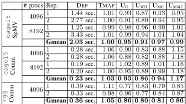
Table I presents a summary of the improvements achieved by the mapping algorithms in our experiments. For each allocation and part number, we calculate the geometric mean of the execution times obtained with the mapping methods on all graphs. The table shows the geometric mean of the
TABLE I: Average improvements of the mapping algorithms on communication-only applications and SpMV kernel that runs for 500 and 1000 iterations for the first and second allocations, respectively.
# procs Rep. DEF TMAP UG UWH UMC UMMC
cage15 SpMV 40961 1.44 sec. 1.01 0.93 0.87 0.93 0.95 2 2.77 sec. 1.00 0.91 0.89 0.94 0.95 81921 1.25 sec. 0.99 0.98 0.96 0.99 1.01 2 3.43 sec. 1.01 0.99 0.94 1.01 1.04 Gmean 2.03 sec. 1.00 0.95 0.91 0.97 0.99 cage15 Comm 40961 0.28 sec. 1.06 0.90 0.83 0.88 1.15 2 0.28 sec. 1.06 0.88 0.82 0.88 1.18 819212 0.19 sec.0.20 sec. 1.01 1.02 0.89 1.011.00 0.95 0.89 0.99 1.161.18 Gmean 0.23 sec. 1.03 0.93 0.86 0.94 1.17 rgg Comm 40961 0.39 sec. 1.11 0.77 0.83 0.79 0.85 2 0.33 sec. 0.98 0.96 0.77 0.84 0.87 Gmean 0.36 sec. 1.05 0.86 0.80 0.81 0.86
other algorithms. The average for all allocations and part
numbers are given at the bottom of the table. Overall, UWH
improves the cage15 SpMV kernel time by 4–13%, whereas the improvements for the communication-only cage15 and
rgg applications are 14% and 20%, respectively, w.r.t. DEF.
V. CONCLUSION
We have proposed fast and high quality topology-aware task mapping methods that use graph models. We have compared the proposed methods with some other graph-based algorithms from the literature and with a default method used in Nersc’s Hopper Supercomputer. The experiments showed that on a set of 25 matrices from the UFL collection, the proposed methods obtained high quality mappings in a very short time for the target system. The experiments with 4096 processors revealed significant improvements on the mapping metrics compared to the Hopper’s default mapping. These improve-ments yield a 43% performance improvement on one case for a communication-only application and a 23% improvement on the SpMV performance. Overall, with 4096 and 8192 proces-sors, the proposed algorithms improve the performance of the SpMV kernel and the communication-only applications by 9% and 14%, respectively. We also evaluated the metrics according to their correlation with the performance. For the applications with a large communication volume, our analysis revealed that the weighted hop metric is the most dominant one, and for those with smaller messages, the average message congestion is a good metric that correlates with the performance.
VI. ACKNOWLEDGMENT
This work was supported in parts by the DOE grant DE-FC02-06ER2775; by the NSF grants CNS-0643969, OCI-0904809 and OCI-0904802; and by France ANR project SOLHAR (ANR-13-MONU-0007).
REFERENCES
[1] F. Pellegrini and J. Roman, “Scotch: A software package for static mapping by dual recursive bipartitioning of process and architecture graphs,” in High-Performance Computing and Networking. Springer, 1996, pp. 493–498.
[2] P. Sanders and C. Schulz, “Engineering multilevel graph partitioning algorithms,” in Algorithms–ESA 2011. Springer, 2011, pp. 469–480. [3] G. Karypis, MeTiS: A software package for partitioning unstructured
graphs, partitioning meshes, and computing fill-reducing orderings of sparse matrices version 5.0, University of Minnesota, Department of Comp. Sci. and Eng., Army HPC Research Center, 2011.
[4] ¨U. V. C¸ ataly¨urek and C. Aykanat, PaToH: A Multilevel Hypergraph Par-titioning Tool, Version 3.0, Bilkent University, Department of Computer Engineering, 1999.
[5] M. Deveci, K. Kaya, B. Uc¸ar, and ¨U. V. C¸ ataly¨urek, “Hypergraph parti-tioning for multiple communication cost metrics: Model and methods,” Journal of Parallel and Distributed Computing (to appear), 2014. [6] H. M. Aktulga, C. Yang, E. G. Ng, P. Maris, and J. P. Vary,
“Topology-aware mappings for large-scale eigenvalue problems,” in Euro-Par 2012 Parallel Processing. Springer, 2012, pp. 830–842.
[7] H. Kikuchi, B. Karki, and S. Saini, “Topology-aware parallel molecular dynamics simulation algorithm,” in Intl Conf Parallel & Distributed Proc Tech & Applications, 2006.
[8] A. Bhatele, L. V. Kale, and S. Kumar, “Dynamic topology aware load balancing algorithms for molecular dynamics applications,” in 23rd Intl Conf Supercomputing. ACM, 2009, pp. 110–116.
[9] W. M. Brown, T. D. Nguyen, M. Fuentes-Cabrera, J. D. Fowlkes, P. D. Rack, M. Berger, and A. S. Bland, “An evaluation of molecular dynamics performance on the hybrid Cray XK6 supercomputer,” in Intl Conf Computational Science (ICCS), 2012.
[10] F. Gygi, E. W. Draeger, M. Schulz, B. de Supinski, J. Gunnels, V. Austel, J. Sexton, F. Franchetti, S. Kral, C. Ueberhuber, and J. Lorenz, “Large-scale electronic structure calculations of high-Z metals on the BlueGene/L platform,” in ACM/IEEE Conf Supercomputing, 2006. [11] G. Almasi, S. Chatterjee, A. Gara, J. Gunnels, M. Gupta, A. Henning,
J. Moreira, and B. Walkup, “Unlocking the performance of the Blue-Gene/L supercomputer,” in ACM/IEEE Conf Supercomputing, 2004. [12] H. Yu, I.-H. Chung, and J. Moreira, “Topology mapping for Blue Gene/L
supercomputer,” in ACM/IEEE Conf Supercomputing, 2006.
[13] J. A. Pascual, J. Miguel-Alonso, and J. A. Lozano, “Optimization-based mapping framework for parallel applications,” Journal of Parallel and Distributed Computing, vol. 71, no. 10, pp. 1377–1387, 2011. [14] M. Deveci, S. Rajamanickam, V. Leung, K. T. Pedretti, S. L. Olivier,
D. P. Bunde, ¨U. V. C¸ ataly¨urek, and K. D. Devine, “Exploiting geometric partitioning in task mapping for parallel computers,” in 28th IPDPS, Phoenix, AZ, 2014.
[15] T. Hoefler and M. Snir, “Generic topology mapping strategies for large-scale parallel architectures,” in 25th ACM Supercomputing, 2011. [16] A. Bhatele, G. Gupta, L. Kale, and I.-H. Chung, “Automated mapping
of regular communication graphs on mesh interconnects,” in Intl Conf High Performance Computing, 2010.
[17] S. W. Bollinger and S. F. Midkiff, “Heuristic technique for processor and link assignment in multicomputers,” IEEE Trans Comput, vol. 40, no. 3, pp. 325–333, 1991.
[18] I.-H. Chung, C.-R. Lee, J. Zhou, and Y.-C. Chung, “Hierarchical mapping for HPC applications,” in Workshop Large-Scale Parallel Processing, 2011, pp. 1810–1818.
[19] T. Chockalingam and S. Arunkumar, “Genetic algorithm based heuristics for the mapping problem,” Computers and Operations Research, vol. 22, no. 1, pp. 55–64, 1995.
[20] C. Walshaw and M. Cross, “Multilevel mesh partitioning for heteroge-neous communication networks,” Future generation computer systems, vol. 17, no. 5, pp. 601–623, 2001.
[21] F. Pellegrini and J. Roman, “Experimental analysis of the dual recursive bipartitioning algorithm for static mapping,” LaBRI, URA CNRS 1304, Univ. Bordeaux I, Tech. Rep. TR 1038-96, 1996.
[22] A. Bhatele, T. Gamblin, S. H. Langer, P. Bremer, E. W. Draeger, B. Hamann, K. E. Isaacs, A. G. Landge, J. A. Levine, V. Pascucci, M. Schulz, and C. H. Still, “Mapping applications with collectives over sub-communicators on torus networks,” in High Performance Computing, Networking, Storage and Analysis (SC), 2012. IEEE. [23] A. Bhatele, N. Jain, K. E. Isaacs, R. Buch, T. Gamblin, S. H. Langer,
and L. V. Kale, “Optimizing the performance of parallel applications on a 5D torus via task mapping,” in IEEE International Conference on High Performance Computing. IEEE Computer Society, Dec. 2014. [24] S. H. Bokhari, “On the mapping problem,” IEEE Trans Comput, vol.
100, no. 3, pp. 207–214, 1981.
[25] C. Albing, N. Troullier, S. Whalen, R. Olson, and J. Glensk, “Topology, bandwidth and performance: A new approach in linear orderings for application placement in a 3D torus,” in Cray User Group (CUG), 2011. [26] C. M. Fiduccia and R. M. Mattheyses, “A linear-time heuristic for improving network partitions,” in 19th Design Automation Conf., 1982. [27] B. Kernighan and S. Lin, “An efficient heuristic procedure for
partition-ing graphs,” The Bell System Technical Journal, Feb 1970.
[28] M. A. Heroux, R. A. Bartlett, V. E. Howle, R. J. Hoekstra, J. J. Hu, T. G. Kolda, R. B. Lehoucq, K. R. Long, R. P. Pawlowski, E. T. Phipps et al., “An overview of the trilinos project,” ACM Transactions on Mathematical Software (TOMS), vol. 31, no. 3, pp. 397–423, 2005.