CDGPS-based relative navigation for multiple spacecraft

CDGPS-Based Relative Navigation for

Multiple Spacecraft

by

Megan Leigh Mitchell

Bachelor of Science Aerospace Engineering

University of Texas at Austin, 2000

AERO

Submitted to the Department of Aeronautics and Astronautics

in partial fulfillment of the requirements for the degree of

Master of Science Aeronautics and Astronautics

at the

MASSACHUSETTS INSTITUTE OF TECHNOLOGY

June 2004

@

Massachusetts Institute of Technology 2004. All rights reserved.

A uthor ... .....

Department of Aeronautics and Astronautics

May 17, 2004

Certified by...

Jonathan P. How

Associate Professor

Thesis Supervisor

Accepted by

Edward M. Greitzer

Chairman, Department Committee on Graduate Students

MASSACHUSETTS INSTITUTE OF TECHNOLOGY

J U

L 0 12004

LIBRARIES

CDGPS-Based Relative Navigation for

Multiple Spacecraft

by

Megan Leigh Mitchell

Submitted to the Department of Aeronautics and Astronautics on May 17, 2004, in partial fulfillment of the

requirements for the degree of

Master of Science Aeronautics and Astronautics

Abstract

This thesis investigates the use of Carrier-phase Differential GPS (CDGPS) in relative navigation filters for formation flying spacecraft. This work analyzes the relationship between the Extended Kalman Filter (EKF) design parameters and the resulting estimation accuracies, and in particular, the effect of the process and measurement noises on the semimajor axis error. This analysis clearly demonstrates that CDGPS-based relative navigation Kalman filters yield good estimation performance without satisfying the strong correlation property that previous work had associated with "good" navigation filters. Several examples are presented to show that the Kalman filter can be forced to create solutions with stronger correlations, but these always result in larger semimajor axis errors. These linear and nonlinear simulations also demonstrated the crucial role of the process noise in determining the semimajor axis knowledge. More sophisticated nonlinear models were included to reduce the propa-gation error in the estimator, but for long time steps and large separations, the EKF, which only uses a linearized covariance propagation, yielded very poor performance. In contrast, the CDGPS-based Unscented Kalman relative navigation Filter (UKF) handled the dynamic and measurement nonlinearities much better and yielded far superior performance than the EKF. The UKF produced good estimates for scenar-ios with long baselines and time steps for which the EKF would diverge rapidly. A hardware-in-the-loop testbed that is compatible with the Spirent Simulator at NASA

GSFC was developed to provide a very flexible and robust capability for

demonstrat-ing CDGPS technologies in closed-loop. This extended previous work to implement the decentralized relative navigation algorithms in real time.

Thesis Supervisor: Jonathan P. How Title: Associate Professor

Acknowledgments

First I thank my advisor, Prof. Jonathan How, for his guidance, lessons, humor and patience throughout my time at MIT. This research was supported by the Na-tional Science Foundation Graduate Research Fellowship Program and NASA Grants

#NAG3-2839, #NAG5-10440, #NCC5-704, and #NCC5-729. Collaboration and

dis-cussion with Dr. Oliver Montenbruck, Prof. Terry Alfriend, Rich Burns, and many other people at NASA GSFC has been helpful in steering my work. Many of my col-leagues at MIT, including Louis Breger, Arthur Richards, Ian Garcia, and Ellis King, have been gracious in offering their insight into technical issues that arose in my work. The support of these and many other MIT friends has made this journey memorable and enjoyable. To my dear friends back in the great State of Texas, thank you for all the calls and letters. I am grateful for my parents, whose love and encouragement helped me get where I am, and for my brother, Stuart, who should know that he is an inspiration to me. Above all, I thank my Heavenly Father, for it was His strength, and not my own, that enabled me to complete this work.

Contents

surements

2.1 The Extended Kalman Filter . . . . 2.2 System Dynamics . . . .

2.2.1 Orbital Mechanics . . . .

2.2.2 Clock Dynamics . . . . 2.2.3 Carrier Phase Biases . . . . 2.2.4 System Dynamics Summary . . . .

2.3 Measurement Update: Carrier Differential GPS . . . . 2.3.1 A Review of Global Positioning System Basics

3 5 6 10 13 15 15 17 18 CDGPS Mea-21 22 26 26 32 33 33 34 34

2.3.2 Raw GPS Measurements . . . . 2.3.3 Differential Carrier Phase Measurements and Relative State 2.3.4 A Summary of Measurement Equations . . . .

2.4 Sum m ary . . . .

3 Noise and Navigation Accuracy for CDGPS Filters

3.1 Relating Navigational Errors to Semimajor Axis Error . . . . 3.2 Semimajor Axis Accuracy from a Cartesian Filter Output . . 3.3 A Linear Planar Model . . . .

3.3.1 Three LPM Examples for Correlation Demonstrations

3.3.2 Discussion of Three LPM Examples . . . . 3.3.3 LPM Simulations with

Q

3.4 Agreement with Analytical Work . . . .

3.5 A Nonlinear GPS Model . . . . 3.5.1 NGM Simulations with

Q

3.6 Summary of Noise and Navigation Accuracy . . . . 4 The Unscented Kalman Filter for Relative Orbital Navigation

4.1 Nonlinearity in Relative Orbital Dynamics . . . . 4.2 The Unscented Kalman Filter . . . . 4.2.1 The Standard Form of the UKF . . . .

4.2.2 The Additive Form of the UKF . . . . 4.2.3 The Square Root Form of the UKF . . . . 4.2.4 Comparison of Additive and Square Root UKF's . . . .

4.3 EKF versus UKF for Relative Navigation . . . .

4.3.1 Summary of Simulations to Compare EKF and UKF . . . . . 4.3.2 Comparison for Single Baseline, as Time Step Increases . . .

4.3.3 Comparison as Baselines Increase . . . . 4.3.4 Comparison for FreeFlyerTM and GSFC simulations . . . . .

4.4 A Final Exam ple . . . . 4.5 Sum m ary . . . .. . . .. . . 35 37 38 39 41 . . . . 42 . . . . 47 . . . . 48 . . . . 52 . . . . 57 . . . . 58 . . . . 63 . . . . 68 . . . . 69 . . . . 74 77 78 79 80 81 84 85 87 88 91 93 93 96 97

5 Development of a Closed Loop Navigation System 5.1 Original and Updated Navigation Systems . . . .

5.2 Real Time Estimation ...

5.3 Receiver Monitor Code Changes ...

5.4 Hardware Closed Loop Navigation Tests . . . . 5.4.1 Closed Loop Test Setup . . . . 5.4.2 Closed Loop Demonstrations . . . .

5.4.3 Future Work for Closed Loop Demonstrations

Architecture 99 100 . . . 105 . . . 109 . . . 110 . . . 111 ... 111 ... 119 6 Conclusion 6.1 Thesis Contributions . . . . 6.2 Future W ork . . . . A Reference Frames Bibliography 121 121 123 125 129

List of Figures

1-1 Illustration of a Formation Flying Mission . . . . 16

2-1 Kalman Filter Process . . . . 22

2-2 Relative Navigation Diagram . . . . 30

3-1 Semimajor Axis Contour Plot, Theoretical . . . . 46

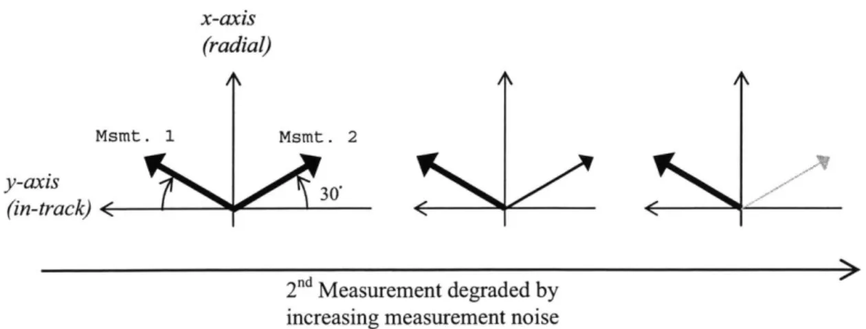
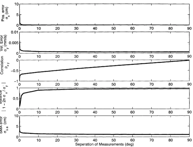
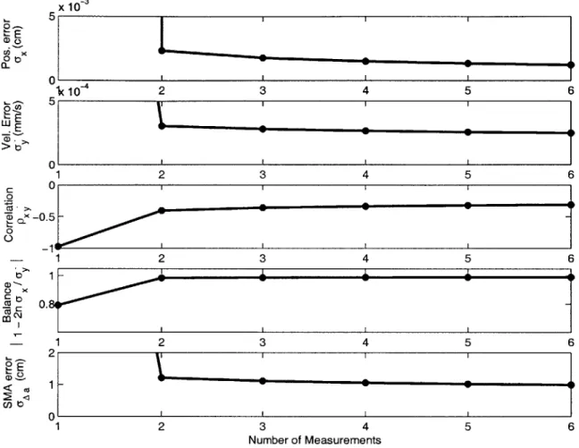
3-2 Diagram of LPM Example with Degraded Measurement . . . . 53

3-3 Diagram of LPM Example with Aligned Measurement . . . . 53

3-4 Diagram of LPM Example with Multiple Measurements . . . . 53

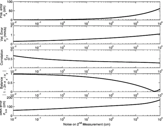
3-5 Results from LPM Example with Degraded Measurement . . . . 55

3-6 Results from LPM Example with Aligned Measurement . . . . 56

3-7 Results from LPM Example with Multiple Measurements . . . . 57

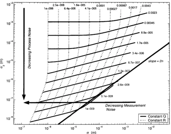
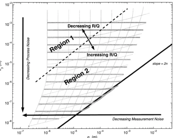
3-8 Contour Plot of

Q,

3-9 Contour Plot of Semimajor Axis for LPM Simulations . . . . 60

3-10 Regions in LPM Simulation Contour Plots . . . . 61

3-11 Contour Plot of Semimajor Axis for LPM Simulations, on Axes of QR 62 3-12 Contour Plot of

Q,

3-13 Predictions for Semimajor Axis and Correlation . . . . 67

3-14 Contour Plot for NGM Simulations: Nonlinear Effects Removed, 0.1 sec tim e step . . . . 71

3-15 Contour Plot for NGM Simulations: Nonlinear Effects Removed, 1 sec tim e step . . . . 71

3-16 Contour Plot for NGM Simulations: Nonlinear Effects Included, 1 sec

. . . . 72

Performance Difference Between UKF-A and UKF-S EKF/UKF Comparison: FreeFlyerTM_{, baseline 100 m} EKF/UKF Comparison: FreeFlyerT M_{, baseline 1 km} EKF/UKF Comparison: FreeFlyerT M, baseline 10 km EKF/UKF Comparison: GSFC, baseline 100 m . . . EKF/UKF Comparison: GSFC, baseline 1 km . . . . EKF/UKF Comparison: GSFC, baseline 10 km . . . A Final EKF/UKF Comparison: FreeFlyerTM, baseline . . . . 87 . . . . 92 . . . . 92 . . . . 92 . . . . 92 . . . . 92 . . . . 92 100 km . . . 96

5-1 Original and Current Simulation Architectures . . . .

5-2 Decentralized Communication between Navigation System Compo-n eCompo-n ts . . . .

5-3 Block Diagram of the Closed Loop Testing Setup . . . .

5-4 Pseudocode for Navigation Executive . . . . 5-5 HITL Navigation Demonstration Setup at GSFC . . . .

5-6 Online Estimation Demonstration, Position Error . . . . 5-7 Online Estimation Demonstration, Velocity Error . . . . 5-8 Online Estimation (with Control Comm.) Demonstration, Position

Error ... ...

5-9 Online Estimation (with Control Comm.) Demonstration, Velocity Error ... ...

5-10 Online Estimation (with Control Comm.) Demonstration, Satellite

Tracking . . . .

5-11 Closed Loop Control Demonstration . . . . A-1

A-2 A-3

ECI and ECEF Reference Frames . . . .

Orbital Elements . . . . LVLH Reference Frame . . . . 4-1 4-2 4-3 4-4 4-5 4-6 4-7 4-8 101 102 103 106 112 114 114 117 117 118 118 126 127 128 time step

List of Tables

3.1 Kalman Filter Elements for LPM Simulations . . . . 49 4.1 UKF-A Algorithm . . . . 83

4.2 UKF-S Algorithm . . . . 86

4.3 Comparison of the Standard Additive and Square Root Forms of the

UKF ... ... 88

4.4 Summary of the Simulations and Results. . . . . 89 5.1 Summary of Code Changes Made to Accommodate Online Estimation

Chapter 1

Introduction

This thesis investigates the use of Carrier-phase Differential GPS (CDGPS) in rel-ative navigation filters for formation flying spacecraft. Previous work successfully developed an Extended Kalman Filter for this purpose [1]. This thesis extends that work by exploring the performance limitations and by explicitly implementing the decentralized form of the navigation filter and executing it in real time. Fundamental performance limits of the filter are explored in an analysis of the relationship between the filter noises and the navigation accuracy. The Extended Kalman Filter is also replaced with an Unscented Kalman Filter that more accurately handles the nonlin-ear dynamics and measurement equations. Finally, closed loop navigation and control experiments conducted at NASA Goddard Space Flight Center (GSFC) advanced the CDGPS-based relative navigation algorithms closer to space flight.

1.1

Motivation for Formation Flying Missions

Flying satellites in autonomously controlled formations is desirable for many space science and military applications [2]. The distributed satellites provide platforms for astrophysical interferometric observation instruments, Earth mapping systems such as synthetic aperture radar, or just distributed Earth observation systems [3]. Flying a formation of satellites increases the ability to distribute scientific sensors over longer baselines, giving better resolution. Furthermore, the geometry of the sensors is not

Fig. 1-1: Illustration of the proposed Orion formation flying mission

fixed by a physical structure, and can be changed with formation maneuvers as the need arises. Ref. [4] includes a list of some of the formation flying missions that have been proposed to take advantage of these features. One such mission, Orion, is a low-cost platform for demonstrating formation flying technologies and is shown in Fig. 1-1.

The dynamics of formation flying are based on the same mathematical models de-veloped for rendezvous and station keeping missions [5]. Unlike these other missions, formation flying emphasizes cooperation between vehicles to meet fuel or maneuver time goals [5, 20]. Though relative navigation algorithms are typically formulated independently of the control objectives, accurate navigation estimates are required

by the controller to make formation flying missions feasible [7].

A key step in precise formation flying is developing a sensor that can be used to

accurately measure the relative positions and velocities of the vehicles in the fleet. Carrier-phase Differential GPS provides an ideal sensor for this relative navigation [8]. The following section highlights some of the recent work to develop CDGPS relative navigation filters for Low Earth Orbit (LEO) missions.

1.2

Previous Work on CDGPS-based

Relative Navigation Filters

This thesis extends the work done by Busse, which presented the design and demon-stration of a relative navigation filter based on CDGPS measurements [1, 9]. This filter was developed for use on formation flying satellites in LEO. An Extended Kalman Fil-ter (EKF) that used nonlinear state propagation and nonlinear measurement update methods was shown to provide a highly accurate estimate. Adaptive techniques for process and measurement noise estimation were implemented as well, and shown to further improve the estimates. Busse demonstrated this algorithm with software and hardware simulations. The software simulations propagated a simple orbital dynamics truth model and used the measurement equations to simulate carrier phase measure-ments. The hardware simulations combined an Orion GPS receiver with a Spirent simulator at NASA GSFC, which generated the RF signals that the receiver would see in LEO. The stored receiver measurements were used to evaluate the filter off-line. The performance of this estimator, with position errors of 1 -2 cm and velocity errors of 0.5 mm/sec, matched or exceeded that of its contemporaries [1, 10, 11]. More recent advances in relative navigation have also been made by Leung and Montenbruck [12]. Extensive work to adapt the GPS receiver for use in LEO has resulted in noise levels of 0.5 mm for carrier phase measurements and 0.07 m/sec for Doppler measurements. When using a receiver with extremely low measurement noise, the relative navigation filter accuracy was reported as 1.5 mm for position and 0.005 mm/sec for velocity. This thesis used the same receivers as Busse, with a slightly revised tracking loop filter.

Formations in near-circular Low Earth orbits with baselines of a kilometer or less have been a starting point for much research in formation flying. However, future scientific goals may require formations in eccentric orbits or with larger baselines. These scenarios represent challenges for the standard LEO CDGPS-based navigation systems [13]. Ref. [14] uses a two-step filter to provide relative navigation for close, elliptical formations. The two-step filter was found to be superior to an iterated

Ex-tended Kalman filter when the initial error was large and when few measurements were available Ref. [15] conducted initial experiments using a CDGPS for large for-mations, between 1 and 500 km. Initial results show that, with an accurate dynamics model, CDGPS may still provide good navigation performance.

Coupling estimation algorithms with control algorithms in closed loop demonstra-tions is another aspect required to prove any navigation system. Some past research has worked towards this goal by incorporating pre-planned thrusts in off-line

analy-sis

[1].

methods that used the Spirent simulator in a study limited to two vehicles.

1.3

Contributions

One of the major goals of this thesis is to understand the fundamental relationships between the dynamic system, the measurements and the filter, as well as any inherent limits in filter performance. This knowledge can hopefully be used to highlight steps to improve formation flying navigation systems. This goal is addressed with several different experiments. Finally, a testbed was developed for demonstrating closed loop navigation and control algorithms.

Chapter 2 provides the basic estimator framework for the GPS measurements and the relative navigation filter. The research in Chapter 3 was motivated by a conjecture in the literature which suggested that the orbital GPS navigation results available to date (our CDGPS results included) may have a fundamental deficiency. The issue is with the semimajor axis knowledge, which is crucial for obtaining good control performance. Ref. [17] presents an analysis of the relationship between semimajor axis error, position and velocity error, and the correlation coefficient between position and velocity error. That analysis suggest that a "good" navigation filter would have a strong correlation (i.e. coefficient near -1) to reduce the semimajor axis error [18]. However, practical experience with CDGPS-based filters has shown this is seldom true, even when the accuracies appear to be very high (typical correlations ~ -0.1). This chapter investigates this issue in detail, showing that the Kalman filter uses a

very different strategy for obtaining good estimates of the semimajor axis than those suggested in [18].

Chapter 3 also explores the relationship between filter accuracy and process & measurement noises. Both linear planar and nonlinear models are used to create plots similar to those in [17] that provide further insights on what types of noise improvements (i.e., using better models to reduce process noise or lower the phase noise of the receiver to reduce the sensor noise) would improve the CDGPS filter accuracy.

Chapter 4 investigates the navigation accuracy in more detail by evaluating an-other variant of the Kalman Filter for nonlinear systems, called the Unscented Kalman Filter (UKF). The UKF was developed to provide better estimation results for non-linear systems [19]. The chapter explores the limitations of an EKF and the benefits of the UKF as the estimation time step increases and the separation between the spacecraft grows. Both of these changes accentuate the nonlinearity in the system.

Simulations using measurements from software models and from hardware tests at NASA GSFC both confirmed that the Unscented filter yields much better perfor-mance for large baselines or long time steps.

While the stand-alone performance of the navigation algorithm is certainly impor-tant, the final measure of success for an estimator is determined by its performance in a closed loop control scenario. A testbed was developed for the estimation algo-rithms described in this research to be connected to control algoalgo-rithms described in Ref. [20]. The closed loop testing can be done with software-only or with hardware-in-the-loop. The software-only simulations are based on truth trajectory created with a high fidelity orbital propagator, and use simulated measurements created from the measurement equations and the truth trajectory. The hardware simulations, which replace the simulated measurements with a Spirent GPS signal simulator and Orion

GPS receiver, were conducted at NASA GSFC. Chapter 5 describes the development

of the testbed architecture required to support these closed loop simulations. This includes the Navigation Executive software that regulates the communication and executes the filter steps. Several simulations that illustrate the development of the

testbed are presented. While the testbed was created to demonstrate the estimation algorithms in this thesis and the control algorithms in Ref. [20], either component can be exchanged in future experiments. The Orion receiver could also be replaced to evaluate the performance of the EKF/UKF estimators with another receiver.

Chapter 2

A Kalman Filter with Relative

Orbital Dynamics and CDGPS

Measurements

In 1960, Robert Kalman introduced a new approach for minimum mean-square er-ror filtering that used state space methods [21]. The Kalman Filter is a recursive scheme that propagates a current estimate of a state and the error covariance matrix of that state forward in time. The filter optimally blends the new information intro-duced by the measurements with old information embodied in the prior state with a Kalman gain matrix. The gain matrix balances uncertainty in the measurements with the uncertainty in the dynamics model [22]. The Kalman filter is guaranteed to be the best filter for a linear system with linear measurements [23]. However, few systems can be accurately modeled with linear dynamics. Shortly after its inception, improvements on the Kalman filter to handle nonlinear systems were proposed. One of the most popular choices, the Extended Kalman Filter, was used in previous work on relative navigation filters in LEO [1]. This chapter begins with a review of the discrete Extended Kalman Filter (EKF) and its application to the relative orbital navigation problem. Next, the mathematical descriptions of the system dynamics and measurement models that are used in the Kalman filter are presented. A review of the pertinent orbital mechanics equations leads to the definition of the system

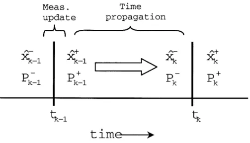
Meas. Time

update propagation

1"kl -k -1 k

-P

P*

P~

P

t

ime-Fig. 2-1: Kalman Filter Process

dynamics model. The equations that relate Carrier Differential GPS measurements to the relative state are the basis for the measurement model in this Kalman Filter. The Kalman Filter, Orbital Dynamics, and GPS Measurements are discussed in this chapter and provide a base for the discussions in later chapters.

2.1

The Extended Kalman Filter

This section presents the equations used in the discrete Extended Kalman Filter (EKF). The dynamics and measurements models used in the Kalman filter are dis-cussed in subsequent sections. The discrete EKF is as a state estimator for systems whose state dynamics model, measurement model, or both may be nonlinear, as in

Eqs. 2.1 and 2.6 [23]. The dynamics model provides the equations to propagate ik,

the estimate of the state x at time k, to time step k+1, producing Rk+1. The measure-ment model then incorporates the new sensor information to update this estimate,

updating the a priori estimate R+ to the a posteriori estimate, + This process

The continuous state x is governed by the dynamics

k(tk) = f(x, U, tk) + W(tk) (2.1)

where u is a known control input, and w(t) is an additive white noise that models the error accumulated by uncertainty in the dynamics during the time step. The power spectral density of this zero mean, white noise process is

Q = E[w(t) w(t)'] (2.2)

To proceed, linear expressions for the dynamics and measurement equations must be formed. In general, this requires knowledge of the probability density function [23], but the EKF approximates the nonlinear function by expanding it in a Taylor series, at each time step, about the current estimate,

F = Of(2.3)

The dynamics are discretized with time step At by forming the state transition matrix,

(bk- eFkAt (2.4)

The cumulative effect of the white noise process w(t) over the time step is captured in the discrete process noise covariance matrix

Qk

j

The vector of measurements, y,

y = h(x, t) + Vk (2.6)

is modeled as a nonlinear function of the state and time, with an additive white noise process v(t) that accounts for uncertainty the sensors and their models. The

measurement noise covariance matrix is defined by

Rk = E[Vk vT] (2.7)

The nonlinear measurement equation is also linearized about the current estimate,

Hk = _(2.8)

Because approximations must be made in the linearization, the EKF is a sub-optimal filter, in the sense that its stability and performance are not guaranteed. Fortunately, the dynamics of orbital motion are fairly simple, and the EKF can have very good performance in space navigation applications [22]. The discrete, linear representation of the system dynamics are

Xk k-1Xk-1 + Wk-1 + Uk-1 (2.9)

The confidence in the current estimate is captured in the state error covariance matrix, P,

Pk = E[Rk T] = E[(Rk - xk)(k - xk)T] (2.10)

where Xk = xk - Xk is the estimation error. The first step in the EKF involves

propagating the state and error covariance forward in time. Eq. 2.9 (with zero process noise) is used to propagate the state estimate. The error covariance is propagated forward using

Pk = (k- ₁-

-

An alternate approach to the time propagation step involves using the nonlinear dynamics equations to propagate the state. A 4th-order Runge-Kutta integration scheme uses the nonlinear state dynamics equation

to find Xk. The state covariance is still propagated with Eq. 2.11, so the state

tran-sition matrix <kb1 must be calculated regardless of whether the linear or nonlinear state propagation is chosen. Previous research found the nonlinear method of state propagation offers significant improvement as both vehicle separation and integration time were increased [1]. Except where noted, the state propagation in this research employs this nonlinear method.

The second step of the filter uses the measurement equation to update the a priori state iR_ to the a posteriori state R+. When a measurement becomes available, the new information provided by the measurement and the previous information captured in the state estimate are combined to form an updated state estimate. The Kalman gain K is the blending gain matrix that is used to weight the importance of the old and new information. The optimum gain matrix is formulated by minimizing the trace of the a posteriori state error covariance matrix Pt, which essentially minimizes the estimation error vector at each time step [23]. The terms in the gain matrix equation include the previous state estimate, the linearized measurement matrix, and the expected noise of the new measurements,

Kk = P-Hk(HkP-HI + Rk) 1 (2.13)

The nonlinear measurement equation is used to update the state estimate

k =R - Kk(yk- hk (k)(.4

Note that the computation of the gain matrix Kk requires the linear measurement

matrix Hk. The covariance is updated after the measurement with

P+= (I - KkHk)P1 (I - KkHk)l + KkRkK T (2.15)

which is the Joseph form of the covariance update whose inherent symmetry makes it numerically stable [24]. This section has introduced the basic equations for the Ex-tended Kalman Filter. The definition of the state x and the development of the state

dynamics equations is presented in Section 2.2. The definition of the measurement vector y and the equations that relate the measurement to the state are presented in Section 2.3.

2.2

System Dynamics

The relative state used in this work includes the quantities of interest for navigation and control, relative position and velocity of the vehicle, as well as several other quantities that included in the augmented state so the filter will function properly. These other quantities, associated with the use of CDGPS, include the clock offset, the clock drift rate, and a carrier phase bias for each GPS satellite that is tracked. The state vector used for relative navigation between two vehicles in this work is

Arij (tk) position vector

Abij(tk) clock offset

Aigj(tk) velocity vector

Xk = Abij(tk) = clock drift (2.16)

A3% carrier phase bias, channel 1

AON carrier phase bias, channel N

where the relative vectors are expressed in the ECEF frame. The relative position and velocity dynamics, addressed in Section 2.2.1, are defined by orbital mechanics equations. The dynamics equations for the clock states for the carrier biases are shown in Section 2.2.2 and Section 2.2.3, respectively.

2.2.1

Orbital Mechanics

This research is focused on using the Kalman Filter to provide relative navigation for formations of spacecraft. There are several methods for computing the relative position and velocity. The absolute states of the Leader and Follower vehicles could be

found and differenced. This has proved inadequate for close formations [1]. Another strategy, used here, calculates the relative state of Follower vehicle, referenced to the position of the Leader vehicle.

The absolute state is used in the process of obtaining GPS measurements and in functions external to navigation and control, so it is also estimated. There are many estimation techniques available to form an absolute state solution [25, 26, 27]. A standard EKF was used in this work to estimate the absolute state. The dynamics used for the absolute state estimation are presented here and are also used in the development of the relative dynamics equations.

Absolute Orbital Motion

Newton's law of gravitation, Eq. 2.17, refines Kepler's observations that planets and other orbiting bodies follow conic section paths [28]. The motion of an orbiting body around a central massive body, i.e., a satellite around the Earth, is governed by

r = -- (2.17)

where r is the position vector of the orbiting body in the ECI frame, and y =

3.986 x 1014$ is the gravitational parameter of the Earth. The reference frames

used in these discussion are defined fully in Appendix A. In the case of an Earth orbiting satellite, there are additional perturbations that may be modeled

r 3 + aJ2+ aD+ aB+ aSRP (2.18)

where the additional acceleration terms, aJ2, aD, aB, and aSRP, model perturbation forces due to a non-spherical earth, aerodynamic drag, 3rd-body effects, and solar radiation pressure.

The acceleration term aJ2 is a first order model of the nonuniform gravitational field that is caused by the oblateness and nonuniform composition of the earth [29, 30]. The oblateness results from the centripetal forces that forces mass outward at the

equator. The nonuniform distribution of mass throughout the earth leads to the nonuniform gravitational field. The deviation from a point mass gravitational model is captured by modeling different spherical harmonics. The J2 term, modeling a

zonal harmonic that represents the Earths equatorial bulge, accounts for the strongest perturbation in the Earth's gravitational field [31]. Higher order harmonics terms are not included in the Kalman filters used in this research. The J2 term is used in some

of the Kalman filer variants examined in this research [32, 33], and is quantified

aJ2 = J2pRe 1 - y (2.19)

.3 - 5z

2 r

where the ECI position vector r = [ x y z ]T and has a length of r. The average

radius of the Earth, Re, is 6378.14 km, and the first zonal coefficient due to the Earth's oblateness, J2, has a value of 0.0010826269 [28].

The acceleration term aD accounts for aerodynamics forces. These forces are caused by the interaction between the atmosphere, whose density is a strong function of altitude and sun exposure, and the surface of the vehicle [28]. The drag term is more significant than the lift force on the blunt body of the spacecraft, so typically only the drag is modeled. The magnitude of the drag force is dependent on the density of the atmosphere, and the drag coefficient, which is determined by the fontal area of the satellite and the in-track velocity of the satellite. Drag has more of an effect on satellites in LEO than satellites in higher orbits, but is generally small. It is not included in this research.

The term aB accounts for the force due to the gravitational field of additional

3rd body masses, such as the Earth's moon. This force is greater for orbits with

high inclination and large eccentricity. The primary orbit this research addresses is a near-circular Low Earth Orbit. The 3rd-body perturbation is not modeled in this research, but may become important for missions with eccentric orbits.

by solar radiation. The effect of this forces is greater for satellites in high orbits.

Solar radiation pressure is not modeled in this research.

An equivalent representation of the Cartesian state is given by a set of orbital elements. The orbital elements are a set of angles and other parameters that describe the orbital ellipse, its orientation with respect to an inertial reference frame, and the position of the spacecraft in the ellipse. A good discussion of orbital elements and the conversion of between Cartesian coordinates and orbital elements is found in Ref. [28]. Several of the elements and associated parameters appear in the discussion of the relative navigation filters in this research, and are thus defined here. The orbital period, T, is

T= 27r a- (2.20)

where a is the semimajor axis of the orbital ellipse. The mean motion of the orbit,

n, is

n =2 (2.21)

The orbital energy, related to the velocity and height of the satellite, and the semi-major axis a of the orbit, is

r ___(2.22)

2 ||r|| 2a

Relative Orbital Motion

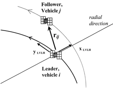
The relative position and velocity terms in the state vector are governed by relative orbital dynamics equations, which can be derived from the absolute orbital dynamics equations. The relative position between vehicles i and

j

j,

Follower,

Vehiclej

radial

direction

Leader,

vehicle i

Fig. 2-2: Relative Position Between Leader and Follower Vehicles

It follows that the relative acceleration is defined by the difference of the two absolute accelerations, with thrust accelerations accounted for with the term uiuj,

Aiy = fj - ii + Aui1 (2.24) Substituting Equations 2.17 and 2.23 into 2.24 gives an expression for the relative dynamics with perturbation terms in the ECI frame,

A r- Ij - ri I ri I 3(ri +

Ari

||ri|3 ||r||2+ 2r2 - Ari3 +|rg 2)

This expression includes the absolute position vector rij of the reference vehicle. The

GPS constellation and the GPS navigation message use the ECEF reference frame,

so ECEF is a natural reference frame for navigation filters using GPS measurements. To transform Eq. 2.26 from the ECI frame to the ECEF frame, a correction term

accounting for the Coriolis effect is added to the dynamics equation,

Ai =r " - IIrI(ri + Arij) + AUz\ + CECEF (2.26)

||ri||3

[

+ Aaj2 + AaD + AaB + AaSRP

where the differential disturbance perturbations have been added, and

CECEF = 2Me x Aigi + Qe X OX X (2.27)

where Qe = 7.292 x 10-, is the rotation rate of the Earth about its axis. Other more sophisticated methods for performing the ECI to ECEF rotation are described in Ref. [28], but the propagation time in the Kalman filter is typically very short, so Eq. 2.27 is usually sufficient. The Jacobian F of the nonlinear relative dynamics equations in Eq. 2.26 is required for the linear state propagation scheme and for the covariance propagation. The linear dynamics matrix for the position and velocity states is given as

where the position and

= 03x3 = I3x3 ' x2 zx 3--0 2Me 0 = -2Q, 0 0 0 0 0 r Q2 e _r2 3 - 3 -1+3 - TQ2 r2 A e zy 3 r2

I

The expressions for relative state dynamics expressed in the LVLH frame are

F Fp1

Fvp FvJ

velocity partitions are

(2.28) (2.29) (2.30) (2.31) (2.32) xz 3 3Q Y r z2 -1+3-T2

also considered. The LVLH dynamics are not used for the state propagation, but are useful for the discussions found in Chapter 3. These equations follow from the assumption that the spacecraft are in close proximity and are in near-circular orbits. The differential perturbation forces are combined into a single acceleration term, f. The linearized relative orbital dynamics for circular orbits expressed in the LVLH frame, also called Hill's or Clohessy-Wiltshire equations [34, 28], are

- 2ny - 3n2X = f (2.33)

jj+ 2nz =

fy

2+

n2z = f2 (2.35)

These equations highlight the relative motion in the radial (x), in-track (y), and cross track directions (z) in the LVLH frame (see Appendix A). The coupling between the radial and in-track directions is apparent in these equations. The out-of-plane motion is modeled as a simple harmonic oscillator. Note that it is well known that the accuracy of these equations degrades rapidly as the separation between vehicles increases or as eccentricity is introduced to the reference orbit.

2.2.2

Clock Dynamics

CDGPS navigation techniques require that time be known with a high degree of

accuracy. The clocks on the local receivers are relatively low quality and unstable, so a clock offset and a clock drift rate must be estimated by including each in the Kalman filter state definition. The dynamics of the clock offset from GPS time, b and the clock drift rate, b, are modeled as

b 0 1 b 0

When the single differences are performed between two vehicles, the relative clock dynamics retain only the differential white noise term,

[

1

A bij j

0 1 Abi1 0

0 0 Abij1J

(2.37)

Thus, in the state propagation step, the clock model will contribute nothing to the state transition matrix, but will introduce terms in the noise covariance model.

2.2.3

Carrier Phase Biases

Each GPS carrier phase measurement includes a bias term. This bias is treated as a constant that must be estimated. A description of the carrier bias is found in Section 2.3.2. The differential biases are modeled as constants,

A)3= 0 (2.38)

2.2.4 System Dynamics Summary

The full relative state is defined as

Xk =

Arij (tk)

Abi (tk) M 7j (tk)

Abij (tk) (2.39)

The carrier biases, A/i,", are constant and are ignored during the state propagation step. A truncated vector which excludes the biases Ao , ,..., A N3 is propagated.

The linearized dynamics of the position, velocity, and clock states are modeled as Fpp 0 Fpv 0 x(t) = 0 x(t) + w + u (2.40) Fvp 0 Fvv 0 0 0 0 0 where

w = OIx4 WAr WAb] (2.41)

- T

u = [1x4 AU 0 (2.42)

The dynamics and process noise models are then discretized as discussed in Sec-tion 2.1.

2.3

Measurement Update: Carrier Differential GPS

2.3.1

A Review of Global Positioning System Basics

The NAVSTAR Global Positioning System (GPS) is a space based, radio navigation system developed, owned, and operated by the United States Department of De-fense. The GPS satellites transmit signals on two carrier frequencies. The civilian Li frequency, 1575.42 MHz, carries a pseudo-random code for timing and contains a navigation message with ephemeris data [35]. GPS positioning is based on the prin-ciple of trilateration, which is the process of ranging off at least three objects with known position to determine a local position. The clocks that are used in the GPS ranging process are low quality, so the time is added as a fourth dimension. Because of the time uncertainty, the four required ranges are not true measures of position, and are thus called pseudoranges.

The standard method of obtaining a pseudorange involves using the navigation information on the code message. Code based pseudorange measurements typically

produce differential accuracies of several meters, which are not sufficient for formation flying missions. Carrier techniques offer much higher accuracy by calculating pseudo-ranges from the phase measurement of the RF carrier wave. If carrier measurements from a mobile receiver and a base station are differenced (forming a CDGPS

mea-surement), the motion can be observed highly accurately. If the base is also moving, as in the case of Leader and Follower vehicles in a satellite formation, the CDGPS observable leads to relative position and velocity [25]. CDGPS measurements are used in this research to provide highly accurate relative navigation. The following section develops the CDGPS based pseudorange equations.

In addition to the code and carrier pseudoranges, a Doppler measurement,which can be related to velocity, is available from the GPS receiver. The Doppler mea-surement is created inside the receiver by differencing carrier phase meamea-surements. Because this is not a truly independent measurement, previous research has found that adding Doppler measurements does not significantly improve the state estimate

[1].

For this reason, the Doppler measurements are not included in this discussion.

2.3.2

Raw GPS Measurements

The code based pseudorange is used to calculate the absolute state. The code phase,

p, is

p, = | - ri| + bi + B"i + i" + vp (2.43) where

||rmi

Bmi. The unmodeled (and unknowable) phenomenon that affect the code phase measurement are included in the noise term, vp. The term Im models the delay imposed on the signal by the ionosphere. This term is modeled as

82.1 x TEC _(2.44)

where TEC is the total electron count on the atmosphere, a varying quantity in-fluenced by, among other things, local solar illumination and sunspot activity. The frequency of the electromagnetic, Fe, and the elevation angle of the GPS satellite m with respect to vehicle i,

'y7n,

The carrier phase pseudorange, similarly relating range, clock states, and iono-spheric delay, is

#'" = ||r"i - ri||+ bi + B"n + O"' - I" + v4 (2.45)

A carrier phase noise term, v4 in Eq. 2.45, replaces the code noise from Eq. 2.43. The

difference in the effect of wave delay seen by the carrier and group delay seen by the code is reflected in the carrier pseudorange in Eq. 2.45 that has an ionospheric delay term that opposite in sign.

The additional term ,37 introduced in the carrier pseudorange is a carrier phase bias. The bias is required to deal with an integer ambiguity in the phase measurement. The distance between the GPS satellite and the vehicle can be expressed as the sum of the carrier phase

#,

d = #+ kA

where A ~ 19.2 cm. The distance viewed as being measured in units of carrier wave-lengths, the fractional part of the distance, which is the carrier phase measurement, is known very accurately. The part of the distance that is covered by the integer mul-tiple of wavelengths cannot be determined immediately from the information in the carrier phase measurement. Fortunately, there are a number of techniques available to determine this integer number. A passive technique called kinematic positioning was used in this research. As the GPS constellation and the spacecraft move relative to each other, the range measurements will change, but the bias remains constant [1]. With measurements collected over time, the biases are then observable and can be estimated. While this technique results in a longer startup time, it is quite simple and the biases do not change after the initial startup period. When new GPS satellites

enter the antenna's field of view, the biases in their measurements can be determined very quickly. Another advantage to this approach is that because the bias estimates are not necessarily required to be integers, the bias estimate can include constant errors, such as those potentially introduced by an antenna line bias or the correlator inside the receiver.

The line-of-sight (LOS) vector is a unit vector whose origin is vehicle i and points towards GPS satellite m,

rmi -r (2.46)

lirmi -ri||

The vectors in the LOS equation refer to the positions of vehicle i at the time of measurement and the GPS satellite m at the time of signal transmission. The mea-surement matrix H includes the LOS vectors for each GPS satellite tracked,

lost

I

HLOS (2.47)

Llost

1j

The Geometric Dilution of Precision (GDOP), indicates the distribution of satellites, GDOP =

[(HOSHLOS

A low GDOP indicates good GPS satellite coverage, which means that measurements

are available in all directions, providing good observability of the state. Conversely, a large GDOP indicates poor coverage and may result in degraded estimates.

2.3.3

Differential Carrier Phase Measurements and Relative

State

When two vehicles in close proximity track the same GPS satellites, the measurement for GPS satellite m taken by vehicle i will see many of the same errors as the mea-surement taken by vehicle

j.

(CDGPS). The carrier differential phase is defined as

#"/ = # - #"(2.49)

where

#O"

#j

j.

by both vehicles. Substituting the Eq. 2.45 into this difference yields an expression

for the carrier differential phase measurement,

A#"|= ||r" - ri|| - |r"i - rj||+ AB + Abij + ABm + AIj + vA (2.50)

The carrier differential phase can be expressed explicitly as a function of the relative state, as defined in Eq. 2.23,

A#b = ||r"i - ril| - ||r"' - (ri + Arij)l + A/3U + Abij + ABU + AI- + vAO (2.51)

As in the equations for relative orbital mechanics, the relative carrier phase mea-surement equation retains the absolute state of the reference vehicle. Also, the error terms introduced for the raw carrier phase measurements have become differential terms. If the vehicles are close, it is reasonable to assume that the terms modeling the GPS satellite clock error and the ionospheric delay cancel,

o#i = ||r"i - rill - ||r m - (ri + Arij)l + o#2 + Abij + vA (2.52)

2.3.4

A Summary of Measurement Equations

The measurement vector, y, contains all the measurements that are used in the Kalman filter. The GPS receiver used in this research tracks up to 12 GPS satellites, so the measurement vector

AOig(tk)

Yk : (2.53)

may include as estimate of the

many as N = 12 differential carrier phase measurements. relative state, the nonlinear measurement equation is

[l~

fil- lfli

(fi +

ZArij)II

+

Abi

+ zAy3% +

L -jN - flj.Nj - (fi + Arij)ll + Abi + AO/3 + Ab N2 AI (f,j Af₇j, jfln) + VAxO

=hk(Rk ) + V

Given an

(2.54)

(2.55)

and the associated Jacobian is

Hk =

[

2.4

Summary

The EKF for CDGPS-based relative navigation described in this chapter was devel-oped and tested by Busse [1], and is the basis for much of the work in this thesis. Chapter 3 investigates the relationships between measurement and process noises and filter performance for this filter. Busse's algorithm was structured to allow real-time, decentralized execution, but he did not implement it that way. Chapter 5 describes the adaptation of this algorithm in a testbed for closed loop navigation and control algorithms.

Chapter 3

Noise and Navigation Accuracy for

CDGPS Filters

Effective design and analysis of a navigation filter must include a detailed evaluation of the filter's performance. Understanding the factors driving the performance and the elements of the system that limit navigation accuracies provides useful information for future improvements. Changing the various elements of the estimator, such as the sensor or dynamics model, can provide new insights into the steps necessary to improve performance. This chapter performs a key step in the estimator evaluation

by investigating the relationship between the Kalman filter design parameters and

the resulting navigational accuracies, and in particular, the roles of the process and measurement noises and their effect on semimajor axis error. Accurate knowledge of semimajor axis error is a dominate factor for control system performance, and thus is functionally the most important navigation parameter [6].

The chapter begins with a review of how semimajor axis error relates to the other navigational errors in our CDGPS-based Kalman filter. The design parameters available in the Kalman filter are reviewed prior to the exploration of their effects. This investigation begins with a linear model that excludes errors introduced by absolute state error, ionosphere, clocks, and carrier phase bias. The goal is to use the linear model to gain insights into the fundamental behavior of the filter before adding other real-world effects.

The linear model is first used to demonstrate that navigation accuracy degrades when the problem statement is changed to force a high correlation between the posi-tion and velocity estimates. This provides a counterexample to a previous conjecture that suggests semimajor axis error can effectively be canceled when there is high correlation between position and velocity error [18]. The example is further used to explore how the filter design parameters affect the navigation accuracy. Finally, the mapping between the simplified, linear simulations and full CDGPS-driven simula-tions is shown to validate conclusions drawn from the linear analysis.

3.1

Relating Navigational Errors to Semimajor Axis

Error

In formation flying missions, accurate knowledge of the difference in semimajor axes, or equivalently, the difference in orbital energy, between the vehicles in the formation is important [7], [17], [18]. A difference in semimajor axes means that the two ve-hicles have different orbital periods and thus they will drift out of formation unless considerable control effort is applied [6].

The output of the CDGPS Kalman filter includes the relative formation state in a Local Vertical Local Horizontal (LVLH) reference frame, which is defined in Appendix A. Understanding the relationship between position and velocity accuracies and semimajor axis accuracy is key to evaluating the output of this type of filter. While Ref. [18] develops the navigation error analysis from absolute state relations, the results can be reformulated for the relative case. The relative navigation error equations, shown below, relate semimajor axis error to position and velocity errors. Note that this discussion is limited to circular reference orbits. The semimajor axis, a, of vehicle i is

1 _ 2 v? (3.1)

ai ri p

where r and v are the position and velocity magnitudes in the Earth Centered Inertial

used to find the difference in semimajor axes of vehicles i and

j,

Aaij _ 2(rj - ri) + 2(vj - vi) (3.2)

n

where the vehicles are assumed to be in circular orbits and close to each other. The relative position and velocity differences in Eq. 3.2 are the differences in the magni-tudes of position and velocity of the two vehicles. If the two vehicles are close and in circular orbits, a reasonable approximation is to assume that the position difference is in the radial direction and the velocity difference is in the in-track direction [34]. The radial, in-track, and cross-track directions define the x, y and z axes of the LVLH reference frame. The relative dynamics in this LVLH reference frame are described

by Hill's equations [34],

-2ny - 3n2_{x = (3.3)}

=+

2nz = fy (3.4)

+ n 2z = f (3.5)

The force-free solution to Hill's equations is

x(t) = Osin nt - 2yo + 3xo cos nt +2o 4xo (3.6)

n n

(

y(t) = cos nt + + 6xo sin nt + yo - - -3o + 6no)t (3.7)

n (n n

z(t) = zo cos nt + -o sin nt (3.8)

n

In terms of relative radial position and in-track velocity, x and

y,

A a 2 2x+ ) = -(6nx + 3)

(-)

n 3n

The differential semimajor axis is directly related to the secular drift term in the solution to Hill's equations, -(6nx + 3y)t, by a factor of - . If the difference in

semimajor axes is zero, there will be no secular drift between the spacecraft. The standard deviation of the differential semimajor axis estimate, UA, follows directly,

as in

[18],

UAa = 2 + 4-? -pyo +

n n (3.10)

The parameters o-, o-, and px are derived from the error covariance matrix for the

relative LVLH state estimate, R,

R =

3;

y

(3.11)

with estimation error x = x

-have the covariance matrix of

E[xj ] =

x, which is assumed to be unbiased, E[i] = 0, and

012 o-x PyX U7x PiXGo:o-X Pe'o-%-x 012 pao-yog piyo ogy P iYU7Y PxX7XO~i 0'?_X p ±o-wo-2 pxyo-o wo (3.12)

Note that if the radial position and in-track velocity are linearly correlated (pxp = -1),

the expression for semimajor axis variance, from Eq. 3.10, reduces to

4 1 1)2

o-se = 2 4o0 -_{X n} -o-zo-g + _n2 20 a? = 2 20-3 - -o-9

n (3.13)

If the position and velocity error are linearly correlated and satisfy

og = 2nor- (3.14)

then the position and velocity errors cancel and there is no error in the semimajor axis estimate. In other words, the two requirements for zero semimajor axis variance

are:

px7 = -1 and o-g = 2no.

which will subsequently be referred to as the correlation and balance requirements. In the examples, the balance is quantified with the balance index,

bal = 1 - 2nor (3.15)

which should be zero when the balance requirement is met.

Note that if, instead, we have Pxp = 0, then the expression for semimajor axis

error reduces to

UAa = 2 4o + oU2 (3.16)

and in this case, oAa will not be zero unless both ox and o- are zero, which is not realistic.

The relationship between a, o-, pxp, and o-Aa is illustrated in Fig. 3-1 [18]. The

x and y axes of the plot are the standard deviations of the position and velocity estimation errors. Contours of constant semimajor axis are shown on the figure. Each contour is associated with a value of Pxp in addition to a level of oAa; several values of px; are shown for each level of oAa. The diagonal line indicates where

u = 2nox. Along the diagonal, the lines of constant semimajor axis experience

a "bump" that increases in size as the correlation tends towards -1. This bump corresponds to increasing cancelation between the error in x and

y

However, many points on the graph are intersected by more than one contour of constant semimajor axis. It is the correlation that determines the specific contour on which the system lies.

The analysis presented above was considered when exploring strategies to improve our CDGPS filter. Any navigation system that is not on the "bump" and does not

10 2 10 -33 10 0.3 10 -- p ,0= -0.9 0.1 -. .. p ,=-0.5 10 10-02 10~ 100 10 102 a (in)

Fig. 3-1: Families of contours of constant semimajor axis are shown on axes of

position and velocity accuracy. For each level of semimajor axis, the contour corre-sponding to three levels of correlation are shown [18].

have high correlation is not taking full advantage of the boost in semimajor axis knowledge that might otherwise be enjoyed. Thus, making changes to meet the balance and correlation requirements should result in improvements to semimajor axis error. Unfortunately, the Kalman filter does not allow independent control over

o-, oa, and p,. Further discussion of the relationship between typical values of a-, and u output from a Kalman filter and corresponding pxi, and oYA is provided in the following section.